A parameter-free, solid-angle based, nearest-neighbor algorithm

Abstract

We propose a parameter-free algorithm for the identification of nearest neighbors. The algorithm is very easy to use and has a number of advantages over existing algorithms to identify nearest-neighbors. This solid-angle based nearest-neighbor algorithm (SANN) attributes to each possible neighbor a solid angle and determines the cutoff radius by the requirement that the sum of the solid angles is $4\pi$. The algorithm can be used to analyze 3D images, both from experiments as well as theory, and as the algorithm has a low computational cost, it can also be used “on the fly” in simulations. In this paper, we describe the SANN algorithm, discuss its properties, and compare it to both a fixed-distance cutoff algorithm and to a Voronoi construction by analyzing its behavior in bulk phases of systems of carbon atoms, Lennard-Jones particles and hard spheres as well as in Lennard-Jones systems with liquid-crystal and liquid-vapor interfaces.

I Introduction

In most studies of many-particle systems, one is confronted with the task of determining the nearest neighbors of a particle, or set of particles. Interestingly, while identifying nearest neighbors is an important component of various analyses, and is sometimes even needed to evaluate interaction potentials, there is no unique definition of a nearest neighbor and, as a result, what one defines as a nearest neighbor is typically dependent on the question at hand. The two most common algorithms for determining nearest neighbors are i) a fixed-distance cutoff and ii) a Voronoi construction Okabe et al. (2000). However, many extensions, and other definitions have been used as well, see for instance Refs. Knuth (1968); Peter Wilcox Jones and Rokhlin (2011).

A fixed-distance cutoff is the obvious choice in simulations with particles interacting through a short-range potential, where each nearest neighbor is an interaction partner and the cutoff distance corresponds to the interaction range. Additionally, fixed-distance cutoffs have also been used in determining nearest neighbors for structural analyses such as calculating bond-order parameters in nucleation studies (e.g. see Ref. ten Wolde et al. (1996a)). However, in these cases, the “fixed-distance” is not well defined. Arguably, the first minimum of the pair correlation function $g(r)$ (also known as radial distribution function) is a reasonable choice for the cutoff, as it relates to the neighbors in the first coordination shell. However, the precise location of this minimum depends on both the system’s details and thermodynamic conditions and therefore must be determined every time either one is changed. Additionally, the cutoff is defined for the entire system and, as such, is not appropriate for systems with large density gradients, such as occur naturally in nucleation studies, in systems in the presence of gravity or in systems with interfaces.

In contrast, a Voronoi construction Okabe et al. (2000) is based on purely geometric constraints and is parameter free. In addition to identifying nearest neighbors, this method can be used to determine geometric properties like edges and faces shared between these neighbors - data that are frequently useful for structural analysis and classification. Based on the local environment around a particle, it is more appropriate than a fixed-distance cutoff in the case of density gradients. However, there are also a number of inherent problems with a Voronoi construction, some of which will be discussed in this manuscript. First of all, the method is computationally expensive and hence is rarely used on-the-fly in simulations. More importantly, it is not robust against thermal fluctuations. In a crystal, thermal fluctuations which cause particles to fluctuate around their equilibrium lattice sites can spuriously increase the number of particles which share a small face with the target particle Tanemura et al. (1977); Troadec et al. (1998) and hence increase the number of particles identified as nearest neighbors. There exist extensions to the Voronoi construction which aim to increase the robustness against these fluctuations Tanemura et al. (1977); Hsu and Rahman (1979); Brostow et al. (1998); Bandyopadhyay and Snoeyink (2004); Yu et al. (2005), however, they typically introduce parameters, removing the “parameter free” advantage of the algorithm, and they further increase the computational cost.

Looking at the advantages and disadvantages of both the fixed-distance cutoff and the Voronoi algorithm, we suggest a list of features which a “good” nearest neighbor algorithm should have. Specifically, an algorithm should i) be able to deal with systems with inhomogeneous density, ii) be stable against thermal fluctuations, iii) be parameter free and iv) be computationally inexpensive. In this manuscript, we propose, with these goals in mind, a simple algorithm for the identification of nearest neighbors: the solid-angle based nearest-neighbor algorithm (SANN). This method is based on similar principles to a theory used by Corwin et al. Corwin et al. (2010) which used solid angles to predict the number of nearest neighbors. It is also similar to a Voronoi construction as it does not require tuneable parameters. However, SANN is computationally significantly less expensive than a Voronoi construction. In fact, its computational cost only slightly exceeds that of a fixed-distance cutoff making it suitable for on-the-fly use in simulations. In order to compare our algorithm with the fixed-distance cutoff and Voronoi construction, we apply all three methods to monodisperse hard spheres, Lennard-Jones liquid and fcc crystal bulk phases, the $3$-fold coordinated liquid carbon and graphite phases and the $4$-fold coordinated liquid carbon and diamond phases and compare the set of nearest neighbors obtained with the three methods. On some liquid/solid systems we also compute bond-order parameters and discuss the impact different nearest-neighbor sets have on the bond-order correlator distributions. To conclude, we study liquid-crystal and liquid-vapor Lennard-Jones two-phase systems to test the behavior of SANN at interfaces.

II Method

II.1 Description of SANN method

Figure 1: Definition of the angle $\theta_{i,j}$ associated with a neighbor $j$ of particle $i$. Here, $r_{i,j}$ is the distance between both particles and $R^{(m)}_{i}$ is the neighbor shell radius.

As mentioned in the introduction, there exists no unique definition of a nearest neighbor. Consequently, it comes as no surprise that our SANN algorithm introduces a definition that differs from those of existing algorithms. Yet it has many similarities with the definitions of the fixed-distance cutoff and the Voronoi construction, as it is based on similar concepts.

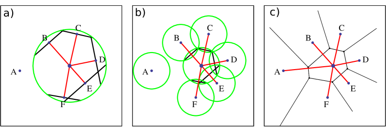
Figure 2: $2d$ comparison of the SANN and Voronoi algorithms. In all three panels we show a central particle with potential nearest neighbors A through F. In panel a) we sketch the SANN algorithm: the green circle shows the shell radius, and particles B through F are identified as nearest neighbors. Note that in all panels the nearest neighbors are indicated with red lines. To facilitate the comparison between a Voronoi construction and the SANN algorithm, in panel b) we make use of the fact that the SANN algorithm is scale free, i.e. $r_{i,j}/R^{(m)}_{i}$ = $(0.5r_{i,j})/(0.5R^{(m)}_{i})$ where $0.5r_{i,j}$ is simply the distance from particle $i$ to the midpoint between $i$ and $j$, and $0.5R^{(m)}_{i}$ is half the shell radius. In panel b) the green circles have a radius equal to the half the shell radius of the center particle, and are centered around each particle; the black lines are constructed by finding the intersection of the green circles and indicate the width of the solid angle between the center particle and each of its neighbors, respectively. Finally, in panel c) we show a Voronoi construction for the same set of particles. Note that the Voronoi construction finds an extra nearest neighbor, i.e. particle A.

Consider a dense system with excluded volume, where we have a particle $i$ located at position $\vec{r}_{i}$ surrounded by particles $\{j\}$. The fixed-distance cutoff defines the nearest neighbors of particle $i$ to be all the particles of $\{j\}$ with a distance to $i$ smaller than the cutoff-distance. However, as mentioned in the introduction, the problem with this definition is in choosing that distance. This is where our SANN algorithm comes into play. For each particle $i$ SANN determines an individual cutoff distance $R^{(m)}_{i}$, which we call the shell radius. It depends on the local environment of particle $i$ and includes its $m$ nearest neighbors. Since the cutoff distance is now a local property, the algorithm is suitable for systems with inhomogeneous densities. For the computation of $R^{(m)}_{i}$ SANN uses a purely geometrical construction, as does the Voronoi tessellation. Thus, the algorithm is parameter-free and scale-free. In the following we describe the geometrical construction and how $m$ and $R^{(m)}_{i}$ are determined.

First, we assume the particles $\{j\}$ surrounding $i$ are known and ordered such that $r_{i,j}\leq r_{i,j+1}$ for all $j$. This relates $R^{(m)}_{i}$ and $m$ in the following manner:

$$r_{i,m}\leq R^{(m)}_{i}<r_{i,m+1}.$$ (1)

Then, starting with the particle closest to $i$ we associate with each potential neighbor $j$ an angle $\theta_{i,j}$ based on the distance between the particles $r_{i,j}=\left|\vec{r}_{j}-\vec{r}_{i}\right|$ and the yet undetermined shell radius $R^{(m)}_{i}$ as depicted in Figure 1.

SANN defines the neighborhood of a particle $i$ to consist of the nearest (i.e. closest) $m$ particles $\{j\}$ such that the sum of their solid angles associated with $\theta_{i,j}$ equals $4\pi$, i.e.

$$4\pi=\sum_{j=1}^{m}2\pi[1-cos(\theta_{i,j})]=\sum_{j=1}^{m}2\pi(1-r_{i,j}/R^{(m)}_{i}).$$ (2)

We point out that while the number $m$ and the shell radius $R^{(m)}_{i}$ are not known yet, they are not independent: once one is known it is straightforward to determine the other. Also note that since the solid angle contribution for a single neighbor is always less than $2\pi$, $m$ must be at least 3.

To visualize this idea imagine each solid angle as a cone with its apex point located at particle $i$ and the cone’s base center located at neighbor $j$. For a complete set of nearest neighbors all those cones stack to fill a spherical volume around $i$ with a radius corresponding to the shell radius $R^{(m)}_{i}$. Obviously, cones are not space-filling (i.e. they don’t stack without gaps), so for the sum of solid angles to equal $4\pi$ some cone overlap does occur.

Combining Eqn. 1 and Eqn. 2 leads to a condition for the determination of the neighbor shell radius,

$$R^{(m)}_{i}=\frac{\sum_{j=1}^{m}r_{i,j}}{m-2}<r_{i,m+1},$$ (3)

where $R^{(m)}_{i}$ refers to the shell radius containing $m$ particles. To solve this inequality, we start with the smallest number of neighbors capable of satisfying Eqn. 2, $m=3$, and increase $m$ iteratively. During each iteration, we evaluate Eqn. 3 and the smallest $m$ that satisfies the equation yields the number of neighbors $N_{b}(i)$ with $R^{(m)}_{i}$ the corresponding neighbor shell radius. It is straightforward to show that the algorithm converges, because the neighbor distance increases monotonically due to the sorting, $r_{i,m+1}\geq r_{i,m}$, and the cutoff radius $R^{(m)}_{i}$ decreases monotonically, $R^{(m+1)}_{i}\leq R^{(m)}_{i}$.

To highlight the differences and similarities between the geometry of the SANN algorithm and that of the Voronoi construction, we show in Figure 2 $2d$-schematics of both. In panel a) we depict the SANN algorithm: the shell radius is show as a green circle, and the red lines connect the central particle to the nearest neighbors determined by SANN, i.e. particles B through F. In panel c) we show the associated Voronoi construction. We note that it identifies all particles A to F as neighbors of the center particle. The Wigner-Seitz cell is indicated with black lines. Neighbor A shares only a small face and is fragile to thermal fluctuations. To compare the Voronoi construction to the SANN algorithm, in panel b) we make use of the fact that the algorithm is scale free, i.e. $r_{i,j}/R^{(m)}_{i}$ = $(0.5r_{i,j})/(0.5R^{(m)}_{i})$ where $0.5r_{i,j}$ is simply the distance from particle $i$ to the midpoint between $i$ and $j$, and $0.5R^{(m)}_{i}$ is half the shell radius. In panel b) the green circles have a radius equal to the half the shell radius of the center particle, and are centered around each particle; the black lines are constructed by finding the intersection of the green circles and indicate the width of the solid angle between the center particle and each of its neighbors, respectively. Hence, one way to picture this method is to picture slowly growing spheres around each particle. When the intersecting planes associated with particle $i$ (the black lines in the plot) yield solid angles summing to 4$\pi$, the shell radius of particle $i$ has been found. This procedure is then repeated for each particle. In the schematic (Figure 2), Particle A is not a neighbor since there is no overlap between the green circle around particle A and green circle around the center particle, hence the fragility problem highlighted in the discussion of the Voronoi construction is not present here. The black lines indicate the width of the solid angles and can be compared to the faces of the Wigner-Seitz cell. However, the faces are not identical to the real Wigner-Seitz cell. In general the faces are either larger or smaller than the real Wigner-Seitz faces. Note that, by definition, SANN extends each face to the shell circle (see Fig. 1), hence, the black lines in the SANN algorithm overlap sometimes, i.e. between particle D and E as well as E and F.

II.2 Algorithm

Following the procedure outlined in the previous section we propose this simple scheme to determine the nearest neighbors of particle $i$:

1. Compute distances $r_{i,j}$ to all potential neighbors $\{j\}$ from $i$.

2. Sort possible neighbors $\{j\}$ by their distance $r_{i,j}$ in increasing order.

3. Start with $m=3$ (i.e. the minimum number of neighbors).

4. Compute $R^{(m)}_{i}=\sum_{j=1}^{m}r_{i,j}/(m-2)$.

5. If $(R^{(m)}_{i}>r_{i,m+1})$, then increment $m$ by $1$ and go back to step 4.

6. Otherwise, $m$ is $N_{b}(i)$, i.e. the number of neighbors for particle $i$, and $R^{(m)}_{i}$ the associated neighbor shell radius.

A C/Fortran implementation of the scheme can be found in the Supplementary Materials SI .

II.3 Algorithm properties

Before comparing our algorithm to the results from a fixed-distance cutoff and a Voronoi construction, we first discuss several inherent properties of our SANN algorithm.

Convergence:

Provided there exist enough neighbors $\{j\}$ of particle $i$ the algorithm converges, because $R^{(m+1)}_{i}<R^{(m)}_{i}$ and all neighbors are sorted such that $r_{m+1}\geq r_{m}$. To proof this, we express $R^{(m+1)}_{i}$ in terms of $R^{(m)}_{i}$:

$$R^{(m+1)}_{i}=R^{(m)}_{i}\Big{[}\frac{m-2+r_{i,m+1}/R^{(m)}_{i}}{m-2+1}\Big{]}.$$ (4)

The definition of $R^{(m+1)}_{i}$ requires that $R^{(m)}_{i}>r_{i,m+1}$, which in combination with Eqn. 4 leads to $R^{(m+1)}_{i}<R^{(m)}_{i}$.

Equal distances neighbors:

The algorithm also ensures that multiple neighbors with equal distance to the center particle are all identified as neighbors. To proof this we show that $R^{(m+1)}_{i}>r_{i,m+i}$, which means that the SANN radius is always larger than each particle distance included. Analogous to the convergence proof, we express $R^{(m+1)}_{i}$ in terms of $r_{i,m+1}$, the latest (and largest) distance included:

$$R^{(m+1)}_{i}=r_{m+1}\Big{[}\frac{R^{(m)}_{i}/r_{i,m+1}(m-2)+1}{m-2+1}\Big{]}.$$ (5)

Again, $R^{(m+1)}_{i}$ requires that $R^{(m)}_{i}>r_{i,m+1}$, which combined with Eqn. 5 leads to $R^{(m+1)}_{i}>r_{i,m+1}$. Therefore, if multiple neighbors share the same distance, all are included.

Pair-wise symmetry:

For both a fixed-distance cutoff and the Voronoi construction, the neighbors are symmetric in the sense that if particle $i$ is a neighbor of $j$, then $j$ is also a neighbor of particle $i$. In SANN, this symmetry is not ensured, because every particle has its own neighbor shell radius. Thus the distance between both particles can be smaller than the shell radius of particle $i$ and larger than that of particle $j$ at the same time; hence, asymmetries can occur. However, we have found that the fraction of asymmetric neighbors is quite small: below 5% for the systems we studied. Moreover, these tend to be those neighbors that are far away, i.e. contribute a small solid angle and are arguably of minor importance for the neighborhood. Therefore, for many applications this might not matter. But in case it does we provide two (arbitrary) ways to make the algorithm ”symmetric”: if $j$ is a neighbor of $i$ but not vice-versa, either a) remove the asymmetric pair, i.e. remove $j$ from the list of neighbors of $i$, or b) complete the asymmetric pair, i.e. add $i$ to the list of neighbors of $j$.

Local volume:

It is possible to assign a local volume to each particle. The Voronoi algorithm has as an obvious choice for the local volume the Wigner-Seitz cell, and by construction the sum of all local volumes adds up to the total system volume. For SANN one can think of many different definitions of a local volume, e.g. related to the shell or cutoff radius, but there is no inherent definition. Consequently, the sum of such local volumes does not by definition equal the system volume. Again, if it is important to attribute a volume to each particle, we can simply (and somewhat arbitrarily) rescale all volumes, such that their sum equals the total volume.

Independence of space dimension:

Although designed for three-dimensional space, we point out that the algorithm is valid without modification for any space-dimension with $d\geq 2$ (and for $d=1$, it is obviously not needed). In particular in higher-dimensional space, e.g. when studying the packing of hyper-spherical particles, easy-to-implement algorithms that go beyond the fixed-distance cutoff are scarce and SANN might be an attractive procedure.

Next-nearest neighbors:

In principle, the algorithm can easily be extended to yield a set of next-nearest neighbors, e.g. neighbor particles with a distance corresponding approximately to the second peak of the pair correlation function $g(r)$. For this task the algorithm is performed twice as follows: in the first run, the nearest neighbors are computed without any modifications. Then all these nearest neighbors are discarded from the list of possible neighbors, and the algorithm is run a second time. Because the algorithm is scale-free, no modification to the algorithm is required, and the next-nearest neighbor shell is obtained. Note that simply increasing the total solid angle to $8\pi$ in Eqn. 2 does not work, as the solid angle contribution of the nearest neighbors would dominate due to the large shell radius $R^{(m)}_{i}$. As we shall see later in the paper, in practice this extension does not work particularly well for finding next-nearest neighbors.

III Simulation Details

Below, we briefly describe the systems and the simulation methods used to produce the test configurations studied in this paper. Moreover, we provides details about the library used for the Voronoi construction and the implementation of our SANN algorithm. At the end of this section we briefly review the bond-order correlators that we use later to perform a structural analysis on some of the systems.

In what follows, we denote the temperature by $T$, the pressure by $P$ and the (number) density by $\rho$. The packing fraction is defined as $\phi=\frac{\pi}{6}\rho d^{3}$, where $d$ is the particle’s diameter. In what follows, $\sigma$ will be the unit of length for both the hard-sphere and the Lennard-Jones systems whereas for carbon we will express the length in Å. All distances presented in the manuscript will be expressed in the appropriate length units.

III.1 Sample preparation

Monodisperse hard-sphere configurations were prepared using an event-driven molecular dynamics simulation in an NVT ensemble with $N=86400$ particles in a cubic box with periodic boundary conditions and with temperature $T=1$, mass $m=1$ and diameter $d=1$. The system was prepared at a packing fraction ($\phi=0.54$) within the solid-liquid coexistence region ($\phi_{f}=0.492$ and $\phi_{s}=0.543$ Noya et al. (2008)) and at a higher packing fraction ($\phi=0.61$) beyond the hard-sphere glass-transition packing fraction ($\phi_{g}=0.58$). In both configurations only 1% of the particles are labeled as solid-like with a $q_{6}$ bond order criterion; note that the $q_{6}$ criterion will be discussed later in the text. For more details on these simulations, we refer the reader to Refs. Sanz et al. (2011) and Valeriani et al. (2011).

The carbon phases were simulated using the LCBOPI⁺ potential Ghiringhelli et al. (2008) at the same conditions as the study on diamond nucleation in Ref. Ghiringhelli et al. (2007), namely $P=30GPa$ and $T=3750K$ for the $3$-fold coordinated liquid and graphite, and $P=85GPa$ and $T=5000K$ for the $4$-fold coordinated liquid and diamond phases. Both conditions correspond to $25\%$ under-cooling with a nucleation free-energy barrier equal to or larger than $\Delta G=25k_{B}T$ (with $k_{B}$ Boltzmann’s constant) preventing spontaneous crystallization of the metastable liquid phase. All systems contained $N=1000$ particles, with the exception of the graphite crystal which had $N=960$ particles. More details on the simulation methods and the semi-empirical interaction potential are given in Ref. Ghiringhelli et al. (2008).

In our discussions of all Lennard-Jones systems, we denote with $T^{*}$ and $P^{*}$ the temperature and pressure in reduced units ($T^{*}=k_{B}T/\epsilon$ and $P^{*}=P\sigma^{3}/\epsilon$), with $\epsilon$ the Lennard-Jones well-depth, and $\rho^{*}=\rho\sigma^{3}$ the density in reduced units. To construct configurations of the Lennard-Jones fcc crystal and liquid phases we performed Monte Carlo simulations in the isothermal-isobaric ensemble for particles interacting via a truncated and shifted Lennard-Jones pair potential Frenkel and Smit (2002); Errington et al. (2003) with a cutoff distance of $2.5$. For both phases, a system of $N=4000$ particles was prepared at the reduced temperature $T^{*}=0.92$ and pressure $P^{*}=5.68$. Under these conditions, which correspond to $20\%$ under-cooling with respect to coexistence, the liquid phase is metastable with respect to the fcc crystal phase. However, a nucleation free-energy barrier of $\Delta G\approx 20k_{B}T$ prevents spontaneous crystallization on simulation time scales ten Wolde et al. (1996b). The two-phase liquid-crystal system was simulated using the same Lennard-Jones potential at the same conditions, but with $N=8000$ particles. The equilibration was biased with a quadratic potential on the number of solid-like particles to prevent the further growth of the crystal phase. See Ref. Frenkel and Smit (2002) for details on biased Monte Carlo simulations and Ref. ten Wolde et al. (1996a) on how to identify solid-like particles. The two-phase liquid-vapor configurations were prepared using the same Lennard-Jones potential and equilibrated using $NVT$ Monte Carlo simulations at reduced temperature $T^{*}=1.0$, number density $\rho^{*}=0.3$, and a system size of $N=5000$ particles. In order to study the liquid-vapor interface, the simulation box was elongated along the x-axis such that the box length in the x direction was 2.5 times as long as the y and z directions. As a result of this simulation box geometry, the resulting liquid-gas interface was perpendicular to the x-axis.

III.2 Voronoi and SANN implementation details

To compute the Voronoi construction, we used the Open Source Computational Geometry Algorithms Library (CGAL Pion and Teillaud (2008)), version 3.7. However, we were only interested in the set of nearest neighbors and not in the additional Voronoi information such as the volume, faces, edges, etc. of the Wigner-Seitz cell. Therefore, it was sufficient and computationally cheaper to perform a Delaunay triangulation, which is the dual of the Voronoi construction. Either construction can be transformed into the other and both yield identical nearest-neighbor sets. We used CGAL’s “exact predicates inexact construction” kernel and included $8$ periodic copies of each particle to emulate periodic boundary conditions. Although CGAL does support $3d$ Delaunay triangulation with $3d$ periodicity, it turned out that the run-time was significantly worse. The particles were inserted sequentially to map CGAL vertex handles and our particle ids.

To speed up the SANN algorithm we made use of a Verlet list Frenkel and Smit (2002) with a long cutoff distance to determine the set of possible neighbors for each particle. Although this method involves a cutoff parameter, we could have chosen a parameter-free algorithm like a binary space partitioning tree or an octree Eberhardt et al. (2010). In general, any domain-decomposition method suffices as long as it provides enough particles for the algorithm to converge.

III.3 Bond-order correlator

In order to identify solid-like particles in some of the systems, we used local bond-order parameters according to Ref. ten Wolde et al. (1996a). The original order parameter described by Steinhardt et al. Steinhardt et al. (1983) is based on the idea of expanding the neighborhood of each particle in a system in terms of a specific set of spherical harmonics, e.g. expanding in terms of the spherical harmonics with $l=3$, $l=4$ or $l=6$, depending on the local symmetry. The algorithm was later refined by ten Wolde et al. ten Wolde et al. (1996a) for the study of nucleation, and has proven to be a useful tool even in the case of higher-dimensional systems van Meel et al. (2009a, b).

To compute the bond-order parameter each particle $i$ is assigned a $(2l+1)$-dimensional complex vector $\vec{q}_{l}(i)$ whose $m$-th component is defined by,

$$q_{l}^{m}(i)=\frac{1}{N_{b}(i)}\sum_{j}Y_{lm}(\vec{\hat{r}}_{ij}),$$ (6)

where $N_{b}(i)$ denotes the number of nearest neighbors, $Y_{lm}(\vec{\hat{r}}_{ij})$ is the set of spherical harmonics of order $l$ with components $-l\leq m\leq l$, $\vec{\hat{r}}_{ij}$ is the unit vector pointing from the center of $i$ to its neighbor $j$, and the sum runs over all neighbors $\{j\}$ of particle $i$. From this we can construct a measure for the neighborhood similarity of two particles,

$$d_{l}(i,j)=\frac{\vec{q}_{l}(i)\cdot\vec{q}_{l}^{*}(j)}{|\vec{q}_{l}(i)|\,|\vec{q}_{l}(j)|},$$ (7)

where the superscript star denotes the complex conjugate. We call the $d_{l}(i,j)$ the local bond-order correlator, which is one when both particles are in an identically ordered environment. To distinguish reliably between solid-like and liquid-like particles, particularly in an under-cooled liquid, additional steps are required to increase the contrast. However, since a change in the neighborhood algorithm already affects this stage of the analysis, we will not follow the procedure to the end, but instead compare the local bond-order correlators.

IV Results

In what follows we apply the proposed algorithm (SANN) to several simulation samples and compare the resulting set of nearest neighbors to the sets obtained from both the fixed-distance cutoff criterion and the Voronoi construction. Moreover, on some systems we perform a structural analysis using bond-order parameters and discuss the impact different nearest-neighbor sets have on the bond-order correlator distributions. We finish by presenting run-times of each algorithm for several simulation samples.

Bulk phases

To start, we compute the nearest-neighbor distribution $P(N_{n})$ for the bulk phases described in Section III.1 using three neighborhood algorithms. For the fixed-distance cutoff, we set the cutoff to the minimum of the pair correlation function, which yields $r_{c}=1.5$ and $r_{c}=1.35$ for the Lennard-Jones liquid and fcc crystal phases, respectively, $r_{c}=2.0$ for all carbon phases, and $r_{c}=1.35$ and $r_{c}=1.3$ for the low- and high-density hard-sphere suspensions.

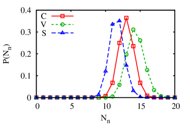
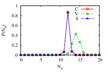
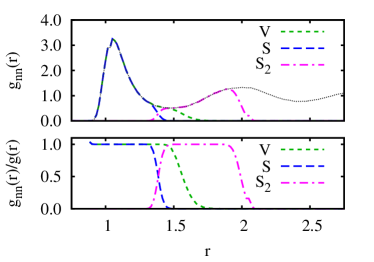
a) b) c) d)

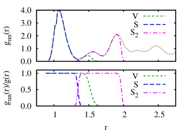
Figure 3: Nearest neighbors distribution $P(N_{n})$ for a Lennard-Jones liquid (panel a) and fcc crystal (panel b) obtained by fixed-distance cutoff ($C$), Voronoi construction ($V$) and SANN considering neighbors belonging to the first coordination shell ($S$). Panels c) and d) plot the pair correlation functions $g(r)$, considering all particles, as a reference (thin grey dotted line), and $g_{nn}(r)$, considering only nearest neighbors (Voronoi ($V$) and SANN ($S$)) and next-nearest neighbors (SANN ($S_{2}$)), for both the liquid (c) and the fcc crystal (d). In addition, their fraction $g_{nn}(r)/g(r)$ is shown.

Figures 3a and 3b depict for the liquid and fcc Lennard-Jones system the nearest-neighbor distribution $P(N_{n})$ computed using fixed-distance cutoff distance ($C$), Voronoi construction ($V$) and our SANN algorithm for nearest neighbors ($S$) and for next-nearest neighbors ($S_{2}$). In both systems, the Voronoi construction identifies more nearest neighbors on average than the fixed-distance cutoff and SANN methods. Its peak in the nearest-neighbor distribution is around $14$ neighbors for both the metastable-liquid and the fcc phases. The fixed-distance cutoff ($C$) exhibits a nearest-neighbor distribution which peaks around $13$ neighbors in the liquid and at $12$ in the fcc crystal, whereas the distribution obtained using the SANN algorithm peaks around $11-12$ neighbors for the liquid and sharply at $12$ neighbors in the fcc crystal. Note that $12$ is also the number that one would expect from a close-packed arrangement of spheres.

In order to get a better understanding regarding the particles which are identified as nearest neighbors in the SANN and Voronoi algorithms, we also compute the pair correlation function using only the nearest neighbors obtained with each method ($g_{nn}(r)$) and compare them to the $g(r)$ of all particles. In the following discussions, we picture the environment around each particle to consist of several shells, each shell associated with a peak in the $g(r)$. Hence, everything up to the first minimum of the $g(r)$ corresponds to the first shell, everything between the first and the second minimum to the second shell and so forth. The fixed-distance cutoff method is not applied here as, by definition, its $g_{nn}(r)$ yields $g(r)$ exactly up to the cutoff radius, after which it is zero. The upper graphs show the pair correlation functions $g_{nn}(r)$ and $g(r)$ for reference, and the lower graphs show the ratio $g_{nn}(r)/g(r)$. At a given distance $r$, the latter ratio gives 1 if all particles at this distance are identified as nearest neighbors, and reduces to zero if none of these particles are considered neighbors. Hence, a steep decrease in the ratio $g_{nn}(r)/g(r)$ indicates few fluctuations in the selection of the neighbors. In addition to the nearest neighbors, the graphs also show results for the next-nearest neighbors obtained from the SANN method ($S_{2}$).

Figure 3c and 3d plots these functions for the Lennard-Jones phases. They show that $g_{nn}(r)$ for the Voronoi construction ($V$) is identical to the reference $g(r)$ up to the first minimum, and in the fcc crystal even slightly beyond that. From the position of the decrease in the $g_{nn}(r)/g(r)$, i.e. slightly to the right of the first minimum in the $g(r)$, we see that the Voronoi algorithm also includes some particles from the second neighbor shell (see upper panels of Figs. 3c and  3d). This behavior originates from fluctuations which cause the Voronoi cell of next-nearest neighbors to occasionally share a small face Troadec et al. (1998). There exist extensions to the Voronoi construction which attempt to increase the robustness of the algorithm to fluctuations Brostow et al. (1998); Bandyopadhyay and Snoeyink (2004); Yu et al. (2005). However, many of them introduce non-inherent parameters and, as such, are not parameter-free. Therefore, we will not consider them here. In contrast to the Voronoi algorithm, the $g_{nn}(r)/g(r)$ associated with the SANN algorithm ($S$) drops to zero at the first minimum for both the liquid and crystal phases and therefore hardly includes any next-nearest neighbors. The SANN algorithm to determine next-nearest neighbors, denoted $S_{2}$, does not yield very precise results. In particular, in the liquid $S_{2}$ finds a few spurious particles from the first neighbor shell and only a fraction of next-nearest neighbors, and in the solid, where it does identify all next-nearest neighbors, it also includes a considerable amount from the third neighbor shell. In both cases this can be attributed to the form of the $g(r)$, i.e. the broadness of the second peak in the liquid, and the closeness of the second and third peaks in the solid. Unfortunately, this is a recurrent problem with trying to use SANN to determine next nearest neighbors, and for this reason $S_{2}$ will not be discussed further in this paper.

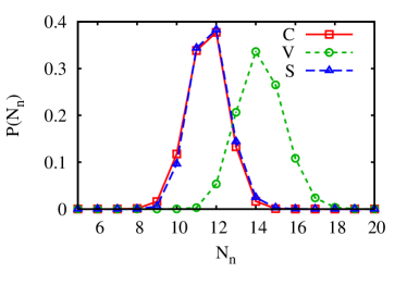
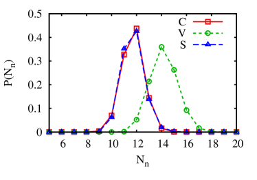
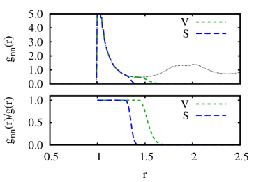
a) b) c) d)

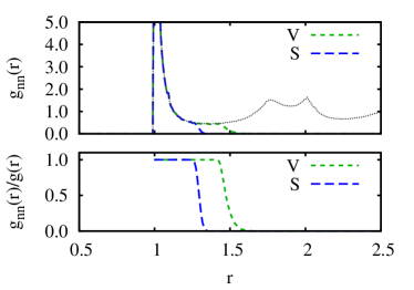
Figure 4: Nearest-neighbor distribution and $g(r)$ as in Figure 3, but for a monodisperse hard spheres system at $\phi=0.54$ (panels a and c) and $\phi=0.61$ (panels b and d).

For both hard-sphere systems studied, i.e. $\phi=0.54$ (fluid) and $\phi=0.61$ (glass), the nearest-neighbor distributions of Figures 4a and 4b computed using the Voronoi construction ($V$) present a peak around $14$ neighbors, given that some of the neighbors from the second shell are included (as shown in Figs. 4c and 4d). In contrast, the distribution obtained using the fixed-distance cutoff ($C$) algorithm and the one obtained with SANN ($S$) are fairly similar (Figs. 4a and 4b) and both peaked around $12$ neighbors for both packing fractions. Again, this is the number one would expect in a close-packed arrangement of spherical particles. From Figures 4c and 4d we see that the pair correlation function for the Voronoi construction is identical to the reference $g(r)$ up to the first minimum. But, as in the Lennard Jones system, it also seems to partially include particles from the second neighbor shell (see upper panels of Figs. 4c and d). In contrast, the $g_{nn}(r)$ computed using SANN drops to zero at the first minimum at both $\phi$’s and does not include next-nearest neighbors.

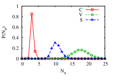
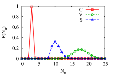
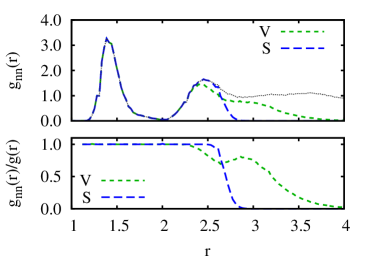
a) b) c) d)

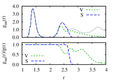
Figure 5: Nearest-neighbor distribution and $g(r)$ as in Figure 3, but for both a $3$-fold coordinated carbon liquid (panels a and c) and graphite crystal (panels b and d).

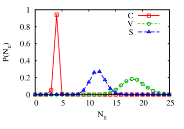
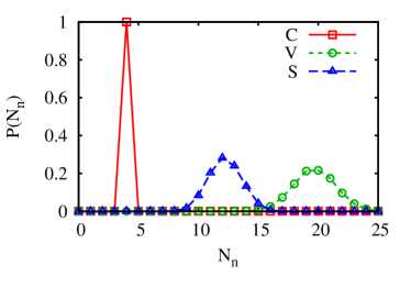
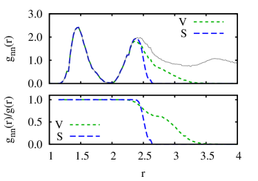
a) b) c) d)

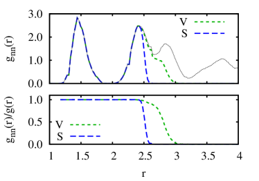
Figure 6: Nearest-neighbor distribution and $g(r)$ as in Figure 3, but for both a $4$-fold coordinated carbon liquid (panels a and c) and diamond crystal (panels b and d).

Figures 5 and 6 depict results for systems consisting of 3-fold coordinated liquid carbon and graphite and 4-fold coordinated liquid carbon and diamond, respectively. In contrast to the Lennard-Jones and hard-sphere systems, carbon is a highly structured network-forming system, even in the liquid phase. It features open structures with few (3 or 4) close-by ordered neighbors: the 3-fold coordinated liquid carbon has a graphite-like structure in the first coordination shell, whereas the 4-fold coordinated liquid carbon has a rather pronounced diamond-like structure in the first coordination shell, shown in the strongly anisotropic angular distribution of the first neighbors. This is reflected in the pair correlation functions $g(r)$ of Figures 5c and 6c, that show a sharp first peak followed by a broad deep minimum: a sign that up to the second neighbor shell the liquid has a structure almost as pronounced as the one of the corresponding solid.

The upper panels of Figures 5 and 6 represent the $P(N_{n})$ computed for the 3-fold coordinated and 4-fold coordinated carbon phases, respectively. The nearest-neighbor distributions from the three methods differ significantly: with the cutoff distance set to the first minimum of the $g(r)$, the fixed-distance cutoff yields a distribution peaked sharply around $3$ (Fig. 5, 3-fold coordinated system) and $4$ (Fig. 6, 4-fold coordinated system) particles both for the liquid and the crystal phases. Counting particles that form chemical bonds, the 3-fold coordinated carbon should have $9$ neighbors within the first two shells ($3$ in the first shell, separated by a distance of about 1.4 Å, and $6$ in the second shell belonging to the same graphite layer), whereas the 4-fold coordinated carbon should have $16$ neighbors within the first two shells ($4$ in the first shell, separated by a distance of about 1.54 Å, and $12$ in the second shell). The SANN algorithm peaks around $10$ (3-fold coordinated systems, Fig. 5) and $12$ (4-fold coordinated systems, Fig. 6) particles for both liquid and crystal phases. Those numbers indicate that SANN includes in each particle’s neighbor list most of the particles belonging to the second coordination shell, as confirmed by the $g(r)$ plots in the lower panels of Figures 5 and  6. The Voronoi construction peaks around $17$ (3-fold coordinated systems, Fig. 5) and $20$ (4-fold coordinated systems, Fig. 6) since it includes particles from the second and third shells. This happens in the liquids, graphite and diamond, as shown by the non-monotonic decay of the Voronoi’s $g_{nn}(r)/g(r)$ that extends well beyond the second minimum in these cases.

To explain the behavior for both the Voronoi construction and the SANN method, we recall that both $3$-fold and the $4$-fold coordinated carbon phases are network-forming open structures. Moreover, graphite forms layers that are several particle diameters apart (with $3.4$ Å  the distance between two layers). This structure affects both algorithms differently; by definition the Voronoi construction searches for neighbors that surround the center particle in all space dimensions, attempting to construct a complete ($3d$) Wigner-Setz cell. For the $4$-fold coordinated carbon phases the Wigner-Seitz cell of the neighbors from the first coordination shell is a fragile tetrahedron, meaning that it is very likely that much further apart particles share a small face. Hence it contains particles from the second and even higher coordination shells. The planar arrangement of neighbors in the $3$-fold coordinated carbon phases forces the Voronoi construction to consider particles from neighboring layers to complete a $3d$ Wigner-Seitz cell; particles that, as one might argue, belong to an entirely different neighborhood. In contrast, SANN does not attempt to complete a $3d$ environment. However, in order to complete its neighborhood with only neighbors from the first coordination shell they must have almost identical distances. This is rarely the case in physical systems and therefore it includes more distant particles as well. Then, however, its neighborhood is dominated by the particles from the first coordination shell, since they are much closer and consequently contribute much larger solid angles in comparison to more distant particles from the second shell. This effect seems to be more pronounced in the diamond crystal phase than in the other carbon phases, and it is the reason why not all particles from the second shell are included.

As an example for this behavior, we depict a few graphite layers in Figure 7, where we color particles identified as neighbors with the Voronoi (panel a) and SANN (panel b) algorithms. Although geometrically correct, the additional neighbors from arguably different neighborhoods identified by the Voronoi construction may distort results for local quantities. Figure 7c presents a top-view of the center layer of panel (b) and shows that the neighborhood identified by SANN includes the complete first and almost complete second neighbor shell.

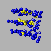
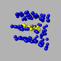
a) b) c)

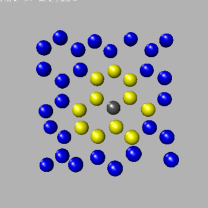
Figure 7: Simulation snapshot of 3-fold coordinated carbon graphite showing the first neighbors (yellow) of a center particle (gray). Surrounding particles that are not part of the neighborhood are shown in blue. a) Voronoi construction; b) SANN algorithm; c) Top-view on the center layer of panel b.

Interfaces

We now apply the three algorithms to two-phase systems with planar interfaces, namely a liquid-crystal and a liquid-vapor Lennard-Jones systems as described in Section III.1. The two phases are arranged in a slab-geometry such that the interfaces are normal to the $x$-direction. For the fixed-distance cutoff we use $r_{c}=1.5$, which corresponds to the minimum of the $g(r)$ for the liquid in the liquid-crystal system; note that the density of this liquid is not the same as the density of the liquid in the liquid-gas system. This choice of $r_{c}$ is arbitrary since there is no way to choose a cutoff which satisfies all four phases simultaneously.

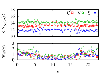
a) b)

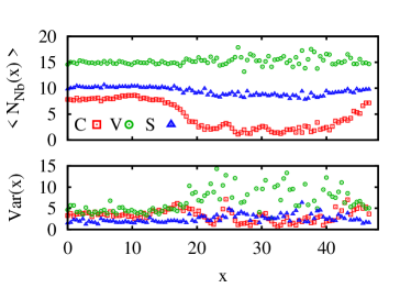
Figure 8: Results for two-phase samples in a slab-geometry, with the two interfaces oriented normal to the $x$-direction. The two phases are a) liquid-crystal and b) liquid-vapor. Note that the densities of the liquid in both cases are not the same. For both samples the upper panel shows, as function of $x$-position, the average number of nearest neighbors, $\Big{<}N_{Nb}(x)\Big{>}$, and the lower panel the corresponding variance, $Var(x)=\Big{<}N_{Nb}^{2}(x)\Big{>}-\Big{<}N_{Nb}(x)\Big{>}^{2}$, for each of the algorithms: fixed-distance cutoff ($C$) with $r_{c}=1.5$, Voronoi construction ($V$) and SANN considering neighbors belonging to the first coordination shell ($S$). Note the different scales on the y-axis.

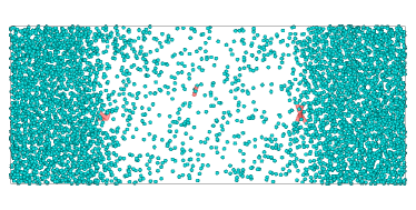
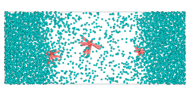
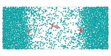
Figure 9: Visual representation of the three algorithms in a two-phase liquid-vapor Lennard-Jones system: fixed-distance cutoff (top), Voronoi construction (center) and SANN (bottom). In each case, we select the same particles and check which neighbors are detected using each algorithm.

In Figure 8 we plot the average number of nearest neighbors $\Big{<}N_{Nb}(x)\Big{>}$ and the corresponding variance $Var(x)=\Big{<}N_{Nb}^{2}(x)\Big{>}-\Big{<}N_{Nb}(x)\Big{>}^{2}$ as a function of $x$ for both systems. As expected, the liquid-crystal interface (Fig. 8 panel a) is barely visible from all three methods and the results are quite similar. However, while the fixed-distance cutoff and SANN methods seem to show a slight increase in $\Big{<}N_{Nb}(x)\Big{>}$ in the crystal phase, this does not appear evident in the Voronoi algorithm. In all cases, the crystal seems to have a slightly lower variance than the fluid. In contrast, the liquid-vapor interface (Fig. 8 panel b) is very well captured by the average number of nearest neighbors (upper panels) computed by the fixed-distance cutoff, whereas the SANN algorithm shows only a slight decrease of the number of nearest neighbors in the vapor phase. The Voronoi algorithm finds even more neighbors in the low-density vapor phase and its standard deviation (lower panel) increases strongly in the vapor phase. This behavior reflects the strong sensitivity of the Voronoi construction to thermal fluctuations. Although $Var(x)$ also fluctuates in the other two methods, the changes are much less pronounced than in the Voronoi case.

To get a better understanding for the nearest neighbors found at the interface and in the vapor phase, in Figure 9 we show a snapshot from the two-phase liquid-vapor system where the vapor phase has been shifted to lie in the center of the box. We have selected three particles (two at the liquid-vapor interface and one in the vapor phase) and have calculated their nearest neighbors using all three algorithms. As expected, in or at the vapor phase the fixed-distance cutoff (upper panel) finds few neighbors when the cutoff is not tuned to the vapor phase. Note that tuning the fixed-distance cutoff for the liquid and vapor phases simultaneously is not possible. The Voronoi algorithm (center panel) detects many neighbors, both for particles at the interface and particularly for particles in the vapor phase. At the interface the SANN algorithm (lower panel) finds neighbors mostly from the interface and liquid and, unlike the Voronoi construction, not far-off in the vapor.

Application to bond-order parameters

Finally, we apply the neighborhood algorithms to investigate their effect on the local bond-order parameters used when studying crystal nucleation. To choose the order of the spherical harmonics in Eqn. 6, we match the symmetry of the spherical harmonics, i.e. $l$, to the symmetry of the crystal under study. For the Lennard-Jones system we use $l=6$ due to the close-packed crystalline structure of the fcc (this is also what is typically used to study hard-sphere systems). In the original article on diamond nucleation Ghiringhelli et al. (2007), $l=3$ was applied to grow both carbon crystal phases since this order parameter is not able to distinguish between graphite and diamond structures. The symmetry $l=3$ was required since only the first neighbor shell was taken into account. However, in the present analysis, both Voronoi and SANN algorithms resulted in neighbor lists which included more than the first neighbor shell. Consequently, the symmetry of the neighborhood changes, and $l=6$ becomes perfectly commensurate with the symmetry of this extended environment. Therefore, we settled for $l=6$ for all systems and set the fixed-distance cutoff in the carbon case to $2.7$ (the minimum after the second peak of the $g(r)$) to include next-nearest neighbors. Also, because bond-order correlators are very sensitive to asymmetries in the nearest neighbor sets and both the fixed-cutoff and the Voronoi construction feature pair-wise symmetry, we decided to enforce this symmetry for SANN, too, by removing asymmetric neighbor pairs. Note that the choice to remove neighbors rather than to add them is arbitrary. The results for the local bond-order correlators distribution $P[d_{6}(i,j)]$ are presented in Figure 10.

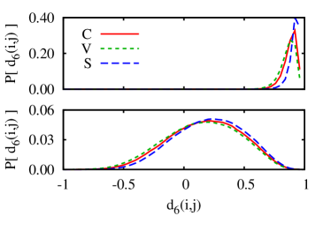
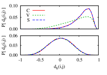
a) b) c)

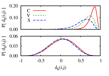
Figure 10: Distribution of the local bond-order correlator $d_{6}(i,j)$ using different neighbor criteria. Panel a) shows results for Lennard-Jones fcc crystal (upper panel) and liquid phases (lower panel), panel b) for the $3$-fold coordinated carbon graphite (upper panel) and liquid (lower panel) phases, and panel c) for the $4$-fold coordinated carbon diamond (upper panel) and liquid (lower panel) phases. For the carbon phases the fixed-distance cutoff distance was set to $2.7$ to include the next-nearest neighbors, as do inherently both the Voronoi and SANN algorithms.

The main criterion for a good order parameter is to have as little overlap as possible between the crystal phase (upper panels) and the (meta-stable) liquid phase (lower panels). As shown in Figure 10a all neighborhood algorithms perform reasonably well for the Lennard-Jones system. However, for the graphite crystal (Fig. 10b upper panel) both SANN and the fixed-cutoff algorithms allow one to distinguish between a liquid and a solid environment, whereas the Voronoi construction shows a severe broadening of the distribution of the graphite, causing a substantial overlap with the liquid’s distribution (lower panel). With such an overlap the bond-order parameters would fail to distinguish between liquid-like and solid-like particles. In the diamond case (Fig. 10c) the SANN algorithm performs worse than the others and again the fixed-distance cutoff works best. In the graphite case the failure of the Voronoi construction can be attributed to the (arguably) spurious neighboring particles located in different graphite layers, as previously discussed (Fig. 7). The behavior of the SANN algorithm in the diamond case finds its origin in that not enough neighbors from the second neighbor shell are included (on average a total of $12$ instead of $16$), and bond-order parameters are particularly sensitive to missing or additional neighboring particles.

Benchmarking

Finally, we measure the run-time of each algorithm for all bulk phases discussed previously. The benchmark was performed on a computer equipped with an Intel Core2 Quad Q9550 processor running at $2.83$ GHz and $4$ GB of DDR2 RAM running at $1066$ MHz. All source code was compiled using the GNU gcc compiler version 4.5.1. The operating system was a $64$-bit OpenSuSE Linux with Kernel 2.6.37. Each algorithm was running single-threaded and computed the neighbor sets for all particles in the system. To improve accuracy whenever the run-time was near our time resolution we measured the total time of $10$ sequential repetitions. All data presented are averages over at least 3 separate program runs.

System	C	V	S	V/C	S/C
Lennard-Jones liquid	25	610	45	24.4	1.8
Lennard-Jones fcc	20	753	48	37.7	2.4
Hard-Spheres $\phi=0.54$	507	14390	1022	28.4	2.0
Hard-Spheres $\phi=0.61$	528	15050	1091	28.5	2.1
Carbon $3$-fold liquid	5	160	8	32.0	1.6
Carbon $3$-fold graphite	5	190	7	38.0	1.4
Carbon $4$-fold liquid	6	153	10	25.5	1.7
Carbon $4$-fold diamond	6	180	9	30.0	1.5

Table 1: Run-times in milli-seconds of the fixed-distance cutoff (C), the Voronoi construction (V) and the SANN algorithm (S), and their ratios V/C and S/C. For details on the system samples we refer to Section III.1, for implementation details to Section III.2, and for the benchmarking procedure to the main text.

The timings are presented in Table 1. Compared to the fixed-distance cutoff the Voronoi construction takes $24.4$ to $38.0$ times longer to compute. In contrast, the computational cost of SANN is only $1.4$ to $2.4$ times that of the fixed-distance cutoff and thereby outperforms the Voronoi construction by an order of magnitude. Therefore, we consider SANN well-suited for application on-the-fly in simulations.

As a final remark we like to point out that timing results are highly implementation dependent and as such should be considered as indications only. On the one hand, the CGAL library used for the Voronoi construction is reasonably fast, but faster implementations may be available. On the other hand, our implementations of the fixed-distance cutoff and the SANN algorithm may have room for optimization, too.

V Conclusion

In this paper we have described an algorithm to compute a particle’s nearest neighbors in an arbitrary many-particle system. The algorithm is similar to a fixed-distance cutoff in that all particles within a cutoff distance are considered nearest neighbors. But rather than using one cutoff for all particles, this algorithm assigns to each particle an individual cutoff distance, thereby making it suitable for systems with inhomogeneous densities, such as gravitational or multi-phase systems. The cutoff distance follows from a geometric requirement, namely that the sum of all solid angles associated with neighboring particles adds up to $4\pi$. Thus, the algorithm becomes parameter-free and scale-free. Though the approach was inspired by the Voronoi construction, it has several advantages over it: the presented algorithm is significantly easier to implement, computationally less expensive and more robust against thermal fluctuations.

We tested the algorithm on a number of bulk phases including supercooled liquid and crystal phases of Lennard-Jones particles, hard spheres and $3$-fold and $4$-fold coordinated carbon. We compared the nearest-neighbor distributions obtained from SANN to both the fixed-distance cutoff criterion and the Voronoi construction. In the case of the Lennard-Jones and hard-sphere phases, our algorithm reproduces very well the nearest-neighbor distribution of a well-tuned fixed-distance cutoff. This is in contrast to a Voronoi construction, which has large fluctuations and as such does not perform as well. For the carbon phases, our algorithm includes the second neighbor shell, like the Voronoi construction, but avoids neighbors in the neighboring graphite layers.

We also examined particles at the interface of two-phase systems, such as Lennard-Jones liquid-vapor and liquid-crystal systems. We find that when two high-density phases coexist, all algorithms give reliable results. However, at the interface between a fluid and a low-density vapor, our algorithm is more robust to thermal fluctuations than the Voronoi construction.

We then employed the neighbor information of all algorithms as input for a bond-order analysis, which is typically used in crystal nucleation studies for the identification of solid-like particles in a supercooled metastable liquid. Comparing the bond-order correlator distributions, we found little difference between the algorithms for the Lennard-Jones system, indicating that all algorithms are suitable for structure analysis of close-packed systems. However, the Voronoi construction failed for the graphite phase due to the identification of spurious neighbors located in different graphite layers, and SANN performed poorly in the diamond phase, due to the fact that not enough neighbors from the second neighbor shell were included. Hence, care has to be taken when applying either one SANN or the Voronoi construction to open structures and network formers. But where the Voronoi construction fails SANN might succeed, and vice-versa.

Finally, we performed benchmarks on the run-time for all algorithms. On all systems tested we found the computational cost of SANN to be at most $2.4$ times that of the fixed-distance cutoff and in all cases it outperformed the Voronoi construction by at least an order of magnitude.

To conclude, when studying a system at several concentrations or a heterogeneous system, the proposed algorithm has the advantage that is does not require tuning a parameter for every concentration/environment. Given the robustness and low computational cost of our algorithm, we argue that SANN is well suited not only for post-analysis, but also on-the-fly in simulations. It reliably identifies the nearest neighbors, and its behavior for graphite and at a two-phase interface suggests its application to situations where the Voronoi construction suffers from distorted polyhedra, like in structural analysis of protein folding trajectories Poupon (2004); Cazals et al. (2006), in DNA-mediated colloidal crystallization Jahn et al. (2010); Noya et al. (2010a), in suspensions of patchy colloids with tetrahedral or octahedral symmetry Saika-Voivod et al. (2011); Noya et al. (2010b, c); Romano et al. (2011) and in water Abascal and Vega (2005). Finally, the SANN algorithm is not only useful for simulation data, but should also be useful in analyzing experimental 3D images, as obtained, for instance, by confocal microscopy or by tomography.