Study of full implicit petroleum engineering finite volume scheme for compressible two phase flow in porous media
Abstract.
An industrial scheme, to simulate the two compressible phase flow in porous media, consists in a finite volume method together with a phase-by-phase upstream scheme. The implicit finite volume scheme satisfies industrial constraints of robustness. We show that the proposed scheme satisfy the maximum principle for the saturation, a discrete energy estimate on the pressures and a function of the saturation that denote capillary terms. These stabilities results allow us to derive the convergence of a subsequence to a weak solution of the continuous equations as the size of the discretization tends to zero. The proof is given for the complete system when the density of the each phase depends on the own pressure.
Key words and phrases:
Finite volume scheme, degenerate problem1. Introduction
A rigorous mathematical study of a petroleum engineering schemes takes an important place in oil recovery engineering for production of hydrocarbons from petroleum reservoirs. This important problem renews the mathematical interest in the equations describing the multi-phase flows through porous media. The derivation of the mathematical equations describing this phenomenon may be found in [6], [10]. The differential equations describing the flow of two incompressible, immiscible fluids in porous media have been studied in the past decades. Existence of weak solutions to these equations has been shown under various assumptions on physical data [4, 10, 11, 12, 13, 17, 18, 24, 25].
The numerical discretization of the two-phase incompressible immiscible flows has been the object of several studies, the description of the numerical treatment by finite difference scheme may be found in the books [5], [27].
The finite volume methods have been proved to be well adapted to discretize conservative equations and have been used in industry because they are cheap, simple to code and robust. The porous media problems are one of the privileged field of applications. This success induced us to study and prove the mathematical convergence of a classical finite volume method for a model of two-phase flow in porous media.
For the two-phase incompressible immiscible flows, the convergence of a cell-centered finite volume scheme to a weak solution is studied in [26], and for a cell-centered finite volume scheme, using a “phase by phase” upstream choice for computations of the fluxes have been treated in [16] and in [8]. The authors give an iterative method to calculate explicitly the phase by phase upwind scheme in the case where the flow is driven by gravitational forces and the capillary pressure is neglected. An introduction of the cell-centered finite volume can be found in [15].
For the convergence analysis of an approximation to miscible fluid flows in porous media by combining mixed finite element and finite volume methods, we refer to [2], [3].
Pioneers works have been done recently by C. Galusinski and M. Saad in a serie of articles about “Degenerate parabolic system for compressible, immiscible, two-phase flows in porous media” ([19], [20], [21]) when the densities depend on the global pressure , and by Z. Khalil and M. Saad in ([22], [23]) for the general case where the density of each phase depends on its own pressure. And for the two compressible, partially miscible flow in porous media, we refer to [9], [28]. For the convergence analysis of a finite volume scheme for a degenerate compressible and immiscible flow in porous media with the feature of global pressure, we refer to [7].
In this paper, we consider a two-phase flow model where the fluids are immiscible. The medium is saturated by a two compressible phase flows. The model is treated without simplified assumptions on the density of each phase, we consider that the density of each phase depends on its corresponding pressure. It is well known that equations arising from multiphase flow in porous media are degenerated. The first type of degeneracy derives from the behavior of relative permeability of each phase which vanishes when his saturation goes to zero. The second type of degeneracy is due to the time derivative term when the saturation of each phase vanishes.
This paper deals with construction and convergence analysis of a finite volume scheme for two compressible and immiscible flow in porous media without simplified assumptions on the state law of the density of each phase.
The goal of this paper is to show that the approximate solution obtained with the proposed upwind finite volume scheme (3.8)–(3.9) converges as the mesh size tends to zero, to a solution of system (2.1) in an appropriate sense defined in section 2. In section 3, we introduce some notations for the finite volume method and we present our numerical scheme and the main theorem of convergence.
In section 4, we derive three preliminary fundamental lemmas. In fact, we will see that we can’t control the discrete gradient of pressure since the mobility of
each phase vanishes in the region where the phase is missing.
So we are going to use the feature of global pressure.
We show that the control of velocities ensures the control of the global
pressure and a dissipative term on saturation in the whole domain regardless of the
presence or the disappearance of the phases.
Section 5 is devoted to a maximum principle on saturation and a well posedness of the scheme which inspired from H.W. Alt, S. Luckhaus [1]. Section
7 is devoted to a space-time compactness of
sequences of approximate solutions.
Finally, the
passage to the limit on the scheme and convergence analysis are performed in section
8. Some numerical results are stated in the last section 9.
2. Mathematical formulation of the continuous problem
Let us state the physical model describing the immiscible displacement of two compressible fluids in porous media. Let be the final time fixed, and let be a bounded open subset of . We set , . The mass conservation of each phase is given in
| (2.1) |
where , and are respectively the
porosity of the medium, the density of the phase and the
saturation of the phase. Here the functions and
are respectively the injection and production terms. Note
that in equation (2.1) the injection term is
multiplied by a known saturation corresponding to the
known injected fluid, whereas the production term is multiplied by the
unknown saturation
corresponding to the produced fluid.
The velocity of each fluid is given by the Darcy law:
| (2.2) |
where is the permeability tensor of the porous medium, the relative permeability of the phase, the constant -phase’s viscosity, the -phase’s pressure and is the gravity term. Assuming that the phases occupy the whole pore space, the phase saturations satisfy
| (2.3) |
The curvature of the contact surface between the two fluids links the jump of pressure of the two phases to the saturation by the capillary pressure law in order to close the system (2.1)-(2.3)
| (2.4) |
With the arbitrary choice of (2.4) (the jump of pressure is a function of ), the application is non-increasing, , and usually when the wetting fluid is at its maximum saturation.
2.1. Assumptions and main result
The model is treated without simplified assumptions on the density of each phase, we consider that the density of each phase depends on its corresponding pressure. The main point is to handle a priori estimates on the approximate solution. The studied system represents two kinds of degeneracy: the degeneracy for evolution terms and the degeneracy for dissipative terms when the saturation vanishes. We will see in the section 5 that we can’t control the discrete gradient of pressure since the mobility of each phase vanishes in the region where the phase is missing. So, we are going to use the feature of global pressure to obtain uniform estimates on the discrete gradient of the global pressure and the discrete gradient of the capillary term (defined on (2.1)) to treat the degeneracy of this system.
Let us summarize some useful notations in the sequel. We recall the conception of the global pressure as describe in [10]
with the -phase’s mobility and the total mobility are defined by
This global pressure can be written as
| (2.5) |
or the artificial pressures are denoted by and defined by:
| (2.6) |
We also define the capillary terms by
and let us finally define the function from to by:
| (2.7) |
We complete the description of the model (2.1) by introducing boundary conditions and initial conditions. To the system (2.1)–(2.4) we add the following mixed boundary conditions. We consider the boundary , where denotes the water injection boundary and the impervious one.
| (2.8) |
where n is the outward normal to .
The initial conditions are defined on pressures
| (2.9) |
We are going to construct a finite volume scheme on orthogonal admissible mesh, we treat here the case where
where is a constant positive. For clarity, we take which
equivalent to change the scale in time.
Next we introduce some physically relevant assumptions on the
coefficients of the system.
-
(1)
There is two positive constants and such that almost everywhere .
-
(2)
The functions and belongs to , In addition, there is a positive constant such that for all ,
-
(3)
, , almost everywhere .
-
(4)
The density is , increasing and there exist two positive constants and such that
-
(5)
The capillary pressure fonction , decreasing and there exists such that .
-
(6)
The function satisfies for and We assume that (the inverse of ) is an Hölder111This means that there exists a positive constant such that for all one has . function of order , with .
The assumptions (H1)–(H6) are classical for porous media. Note that, due to the boundedness of the capillary pressure function, the functions and defined in (2.6) are bounded on .
Let us define the following Sobolev space
this is an Hilbert space with the norm .
3. The finite volume scheme
3.1. Finite volume definitions and notations
Following [15], let us define a finite volume discretization of .
Definition 2.
. An admissible mesh of is given by a set of open bounded polygonal convex subsets of called control volumes and a family of points (the “centers” of control volumes) satisfying the following properties:
-
(1)
The closure of the union of all control volumes is . We denote by the measure of , and define
-
(2)
For any with , then . One denotes by the set of such that the -Lebesgue measure of is positive. For , one denotes and the -Lebesgue measure of . And one denotes the unit normal vector to outward to
-
(3)
For any , one defines and one assumes that .
-
(4)
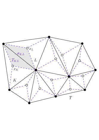
The family of points is such that and, if , it is assumed that the straight line is orthogonal to . We set the distance between the points and , and , that is sometimes called the ”transmissivity” through (see Figure 1).
-
(5)
Let . We assume the following regularity of the mesh :
(3.1)
We denote by the space of functions which are piecewise constant on each control volume . For all and for all , we denote by the constant value of in . For , we define the following inner product:
and the norm in by
Finally, we define the space of functions which are piecewise constant on each control volume with the associated norm
for . Further, a diamond is constructed upon the interface , having , for vertices (see Figure 1) and the -dimensional mesure of equals to .
The discrete gradient of a constant per control volume function is defined as the constant per diamond -valued function with values
And the semi-norm coincides with the norm of , in fact
We assimilate a discrete field on to the piecewise constant vector-function
The discrete divergence of the field is defined as the discrete function with the entires
| (3.2) |
The problem under consideration is time-dependent, hence we also need to discretize the time interval .
Definition 3.
. A time discretization of is given by an integer value and by a strictly increasing sequence of real values with and . Without restriction, we consider a uniform step time , for .
We may then define a discretization of the whole domain in the following way:
Definition 4.
Definition 5.
. Let be a discretization of in the sense of Definition 4. We denote any function from to by using the subscript , and we denote its value at the point using the subscript and the superscript . To any discrete function corresponds an approximate function defined almost everywhere on by:
For any continuous function , denotes the discrete function . if , and is a discrete function, we denote by . For example, .
Let us recall the following two lemmas :
Lemma 1.
Remark 1.
. The lemma 1 gives a discrete Poincaré inequality for Dirichlet boundary conditions on the boundary . In the case of Dirichlet condition on part of the boundary only, it is still possible to prove a discrete Poincaré inequality provided that the polygonal bounded open set is connected.
Lemma 2.
. Let and be a value in depends on and such that and let be a function which is constant on each cell , that is, if then
| (3.3) |
Consequently, if , with , then
| (3.4) |
3.2. The coupled finite volume scheme
The finite volume scheme is obtained by writing the balance equations of the fluxes on each control volume. Let be a discretization of in the sense of Definition 4. Let us integrate equations (2.1) over each control volume . By using the Green formula, if is a vector field, the integral of on a control volume is equal to the sum of the normal fluxes of on the edges (3.2). Here we apply this formula to approximate by means of the values and that are available in the neighborhood of the interface . To do this, let us use some function of . The numerical convection flux functions , are required to satisfy the properties:
| (3.5) |
Note that the assumptions (a), (b) and (c) are standard and they respectively ensure the maximum principle on saturation, the consistency of the numerical flux and the conservation of the numerical flux on each interface. Practical examples of numerical convective flux functions can be found in [15].
In our context, we consider an upwind scheme, the numerical flux satisfying (3.5) defined by
| (3.6) |
where and . Note that the function is non-decreasing, which lead to the monotony property of the function .
The resulting equation is discretized with a implicit Euler scheme in time;
the normal gradients are discretized with a
centered finite difference scheme.
Denote by
and
the
discrete unknowns corresponding to and .
The finite volume scheme is the following set of equations :
| (3.7) |
| (3.8) |
| (3.9) |
| (3.10) |
where the approximation of by an upwind scheme:
| (3.11) |
with and . Notice that the source terms are, for
The mean value of the density of each phase on interfaces is not classical since it is given as
| (3.12) |
This choice is crucial to obtain estimates on discrete pressures.
Note that the numerical fluxes to approach the gravity terms are nondecreasing with respect to and nonincreasing with respect to .
The upwind fluxes (3.6) can be rewritten in the equivalent form
| (3.13) |
where denote the upwind discretization of on the interface and
| (3.14) |
with the set is subset of such that
| (3.15) |
We extend the mobility functions outside by continuous constant functions. We show below (see Prop. 2) that there exists at least one solution to this scheme. From this discrete solution, we build an approximation solution defined almost everywhere on by (see Definition 5):
| (3.16) |
The main result of this paper is the following theorem.
Theorem 1.
Assume hypothesis (H1)-(H6) hold. Let be a sequence of discretization of in the sense of definition 4 such that . Let . Then there exists an approximate solutions corresponding to the system (3.8)-(3.9), which converges (up to a subsequence) to a weak solution of (2.1) in the sense of the Definition 1.
4. Preliminary fundamental lemmas
The mobility of each phase vanishes in the region where the phase is missing. Therefore, if we control the quantities in the -norm, this does not permit the control of the gradient of pressure of each phase. In the continuous case, we have the following relationship between the global pressure, capillary pressure and the pressure of each phase
| (4.1) |
This relationship, means that, the control of the velocities ensures the control of the global pressure and the capillary terms in the whole domain regardless of the presence or the disappearance of the phases. This estimates (of the global pressure and the capillary terms ) has a major role in the analysis, to treat the degeneracy of the dissipative terms .
In the discrete case, these relationship, are not obtained in a straightforward way. This equality is replaced by three discrete inequalities which we state in the following three lemmas.
We derive in the next lemma the preliminary step to proof the estimates of the global pressure and the capillary terms given in Proposition 1 and Corollary 1. These lemmas are first used to prove a compactness lemma and then used for the convergence result.
Lemma 3.
The proof of this lemma is made by R. Eymard and al. in [16]. The proof of this result can be applied for compressible flow since the proof use only the definition of the global pressure.
Lemma 4.
In the incompressible case (see [16]) this kind of estimate is obtained by using the mass conservation equation and under hypotheses ont the relative permeability of the phase, whereas, the compressibility add more difficulties, our approach use only the definition of the function and consequently this lemma can be used for compressible and incompressible degenerate flows.
Proof.
We take the same decomposition of the interface as that proposed by R. Eymard and al. in [16], namely the different possible cases , , and , and the last case and ; where the sets and are defined in (3.15). We establish for the four cases.
First case. If and . We may notice that if the upwind choice is different for the two equations, we have
By definition of in (2.1), there exists some such that
we then get
Second case: The case and
is similar.
Third case: The case and . We have
| (4.5) | ||||
We will distinguish the case and the case .
- (1)
- (2)
which is (4.4) in that case.
Fourth case: The case and is similar of the third case. ∎
Lemma 5.
Proof.
First case. If and . We have
and by definition of there exists some such that , we get then
which gives (4.8). For the discrete estimate (4.9) and by definition of there exists some such that , we get then
which gives (4.9).
Second case. The case and is similar.
The third case and the fourth case can be treated as the cases in the lemma 4. ∎
5. A priori estimates and existence of the approximate solution
We derive new energy estimates on the discrete velocities . Nevertheless, these estimates are degenerate in the sense that they do not permit the control of , especially when a phase is missing. So, the global pressure has a major role in the analysis, we will show that the control of the discrete velocities ensures the control of the discrete gradient of the global pressure and the discrete gradient of the capillary term in the whole domain regardless of the presence or the disappearance of the phases.
The following section gives us some necessary energy estimates to prove the theorem 1.
5.1. The maximum principle
Let us show in the following Lemma that the phase by phase upstream choice yields the stability of the scheme which is a basis to the analysis that we are going to perform.
Lemma 6.
Proof.
Let us show by induction in that for all where . For , the
claim is true for and for all . We argue by
induction that for all , the claim is true up to
order . We consider the control volume such that
and we seek that .
For the above mentioned purpose, multiply the equation in
(3.8) by , we obtain
| (5.1) |
The numerical flux is nonincreasing with respect to (see (a) in (3.5)), and consistence (see (c) in (3.5)), we get
| (5.2) |
Using the identity , and the mobility extended by zero on , then and
| (5.3) |
Then, we deduce from (5.1) that
and from the nonnegativity of , we obtain . This implies that and
In the same way, we prove . ∎
5.2. Estimations on the pressures
Proposition 1.
Proof.
We define the function and . In the following proof, we denote by various real values which only depend on , , , , , , , and not on . To prove the estimate (5.4), we multiply (3.8) and (3.9) respectively by , and adding them, then summing the resulting equation over and . We thus get:
| (5.6) |
where
To handle the first term of the equality (5.6). Let us forget the exponent and let note with the exponent the physical quantities at time . In [22] the authors prove that : for all and such that ,
| (5.7) |
The proof of (5.7) is based on the concavity property of and . So, this yields to
| (5.8) |
Using the fact that the numerical fluxes and are conservative in the sense of (c) in (3.5), we obtain by discrete integration by parts (see Lemma 2)
and due to the correct choice of the density of the phase on each interface,
| (5.9) |
we obtain
The definition of the upwind fluxes in (3.13) implies
Then, we obtain the following equality
| (5.10) |
To handle the other terms of the equality (5.6), firstly let us remark that the numerical fluxes of gravity term are conservative which satisfy and , so we integrate by parts and we obtain
According to the choice of the density of the phase on each interface (5.9) and the definition (3.11) we obtain
Recall the truncations of
with So we obtain
From the following equality and apply the Cauchy-Schwarz inequality to obtain
From the definition of the truncations of , we obtain
| (5.11) |
The last term will be absorbed by the terms on pressures from the
estimate (5.10).
In order to estimate , using the fact that the densities are
bounded and the map is sublinear , we have
then
Hence, by the Hölder inequality, we get that
and, from the discrete Poincaré inequality lemma 1, we get
| (5.12) |
The equality (5.6) with the inequalities (5.8), (5.10), (5.11), (5.12) give (5.4). Then we deduce (5.5) from (4.3). ∎
We now state the following corollary, which is essential for the compactness and limit study.
Corollary 1.
From the previous Proposition, we deduce the following estimations:
| (5.13) | |||
| (5.14) |
and
| (5.15) |
6. Existence of the finite volume scheme
We start with a technical assertion to characterize the zeros of a vector field which stated and proved in [14].
Lemma 7.
([14], p. 529) Assume the continuous function satisfies
for some . Then there exists a point with such that
Proof.
At the beginning of the proof, we set the following notations;
We define the map
| (6.1) | |||
| (6.2) |
Note that is well defined as a continuous function. Also we define the following homeomorphism such that,
where
Now let us consider the following continuous mapping
defined as
According to Lemma 7, our goal now is to show that
| (6.3) |
and for a sufficiently large .
We observe that
for some constants . This implies that
| (6.4) |
for some constants . Finally using the fact that is a Lipschitz function, then there exists a constant such that
Using this to deduce from (6.4) that (6.3) holds for large enough. Hence, we obtain the existence of at least one solution to the scheme (3.8)-(3.9). ∎
7. Compactness properties
In this section we derive estimates on differences of space and time translates of the function which imply that the sequence is relatively compact in .
We replace the study of discrete functions (constant per cylinder ) by the study of functions piecewise continuous in for all , constant in for all volume , defined as
Lemma 8.
Proof.
For and from the definition of , one gets
where and defined as follows
| (7.2) |
| (7.3) |
To handle with the space translation on saturation, we use the fact that is an hölder function, then
and by application of the Cauchy-Schwarz inequality, we deduce
According to [15]), let , , and . We set
We observe that (see for more details [15])
| (7.4) |
To simplify the notation, we write instead of .
Now, denote that
Let us again write , applying again the Cauchy-Schwarz inequality and using the fact that the discrete gradient of the function is bounded (5.13) to obtain
| (7.5) |
To treat the space translate of , we use the fact that the map is bounded and the relationship between the gas pressure and the global pressure, namely : defined in (2.5), then we have
| (7.6) |
furthermore one can easily show that is a , it follows, there exists a positive constant such that
The last term in the previous inequality is proportional to , and consequently it remains to show that the space translate on the global pressure is small with . In fact
Finally, using the fact that the discrete gradient of global pressure is bounded (5.5), we deduce that
| (7.7) |
for some constant .
In addition, we have
where and . By
(7.7), the assumption as and
the boundedness of in , then
the space translates of on are estimated
uniformly for all sequence tend to zero.
In the same way, we prove the space translate for .
∎
We state the following lemma on time translate of .
Lemma 9.
8. Study of the limit
Proposition 3.
Let be a sequence of finite volume discretizations of such that . Then there exists subsequences, still denoted , verify the following convergences
| (8.1) | ||||
| (8.2) | ||||
| (8.3) | ||||
| (8.4) | ||||
| (8.5) | ||||
| (8.6) |
Furthermore,
| (8.7) | ||||
| (8.8) |
Proof.
For the first convergence (8.1) it is useful to introduce the following inequality, for all ,
Applying this inequality to , , from the definition of we deduce
Since tends to zero as , estimate
(7.8) in Lemma 9 implies
that the right-hand side of the above inequality converges to zero as
tends to zero, and this established (8.1).
By the Riesz-Frechet-Kolmogorov compactness criterion, the relative
compactness of in is a
consequence of the Lemmas 8 and
9. Now, the convergence (8.2) in
and a.e in becomes a consequence of
(8.1). Due to the fact that is bounded,
we establish the convergence in . This ensures the following
strong convergences
Denote by . Define the map defined by
| (8.9) |
where are solutions of the system
Note that is well defined as a diffeomorphism, since
and if one of the saturations is zero the other one is one, this
conserves that the jacobian determinant of the map
is strictly negative.
As the map defined in (8.9) is continuous, we deduce
Then, as is continuous, we deduce
and the convergences (8.5) hold.
Consequently and due to the relationship between the pressure of each phase and the global pressure defined in (2.5), then the convergences (8.6) hold
It follows from Proposition 1 that, the sequence is bounded in , and as a consequence of the discrete Poincaré inequality, the sequence is bounded in . Therefore there exist two functions and such that (8.4) holds and
It remains to identify by in the sense of distributions. For that, it is enough to show as :
Let be small enough such that vanishes in for all , then
Now, from the definition of the discrete gradient,
Then,
Due to the smoothness of , one gets
and the Cauchy-Scharwz inequality with the estimate (5.4) in Proposition 1 yield
The identification of the limit in (8.8) follows from the previous convergence. ∎
8.1. Proof of theorem 1
Let be a fixed positive constant and . Set for all
and .
For the discrete liquid equation, we multiply the equation
(3.8) by and sum over and . This yields
where
Making summation by parts in time and keeping in mind that . For all , we get
Since and converge almost everywhere respectively to and , and as a consequence of Lebesgue dominated convergence theorem, we get
Now, let us focus on convergence of the degenerate diffusive term to show
| (8.10) |
Since the discrete gradient of each phase is not bounded, it is not possible to justify the pass to the limit in a straightforward way. To do this, we use the feature of global pressure and the auxiliary pressures defined in (2.5) and the discrete energy estimates in proposition 1 and corollary 1.
Gathering by edges, the term can be rewritten as:
with, by using the definition (2.5),
Let us show that
| (8.11) |
For each couple of neighbours and we denote the minimum of and and we introduce
Remark that
where , , is some point on the segment . Recall that the value of is directed by , so
Define and by
Now, can be written under the following continues form
By the monotonicity of and thanks to the estimate (5.13), we have
Since is continuous, we deduce up to a subsequence
| (8.12) |
Moreover, we have and a.e. on . Consequently, and due to the continuity of the mobility function we have a.e on and in for .
As consequence of the convergence (8.6) and by the Lebesgue dominated convergence theorem we get
And as consequence of the weak convergence on global pressure (8.4), we obtain that
It remains to show that
| (8.13) |
Remark that
Consequently
Applying the Cauchy-Schwarz inequality, and thanks to the uniform
bound on and the convergence
(8.12), we establish (8.13).
To prove the pass to limit of , we need to prove firstly that
where .
In fact. Remark that there exist such as:
since is an Hölder function. Thus we get,
and using the Cauchy-Schwarz inequality and the estimate , we deduce
which shows that as . And from (5.14) in corollary 1, we deduce that there exists a constant where the following inequalities hold:
| (8.14) |
That prove
| (8.15) |
As consequence
| (8.16) |
Rearranging to write
where , , is some point on the segment . using again that the mesh is orthogonal, we can write
As a consequence of the convergences (8.5), (8.6) and by the Lebesgue theorem we get
And as consequence of (8.16),
| (8.17) | ||||
| (8.18) |
Now, we treat the convergence of the gravity term
| (8.19) |
Perform integration by parts (3.3)
Note that the numerical flux is independent of the gradient of pressures and the pass to the limit on is mush simple then the term since the discrete gradient of global pressure is replaced by the gravity vector g. We omit this proof of (8.19).
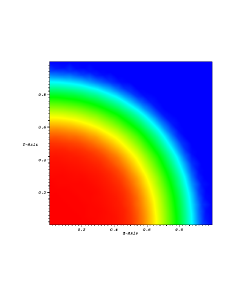
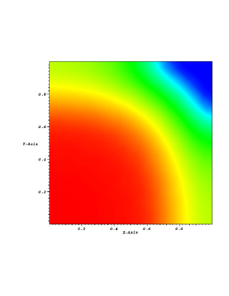
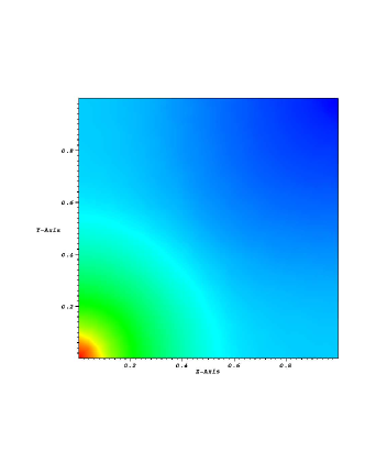
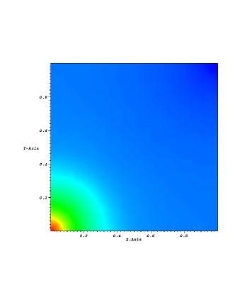
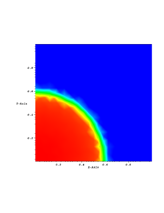
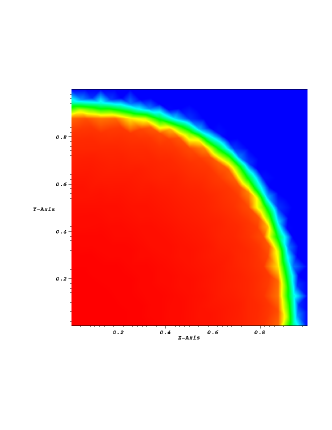
9. Numerical results
In this section we show some numerical experiments simulating the five spot problem in petroleum engineering. A Newton algorithm is implemented to approach the solution of nonlinear system (3.8)-(3.9) coupled with a bigradient method to solve linear system arising from the Newton algorithm process.
We will provide two tests made on a nonuniform admissible grid.
Datas used for the numerical tests are the following :
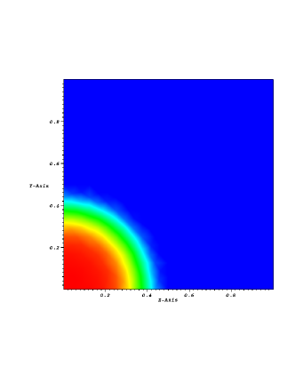
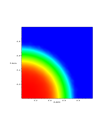
Initial conditions. Initially the saturation of gas is considered to be equal to in the whole domain and the gas pressure is considered to be Pa.
Boundary conditions. The wetting fluid (water) is injected in the left-down corner in the region with a constant pressure equal to Pa. The right-top corner where keeps fluids flow freely at atmospheric pressure where as the rest of the boundary is assumed to be impervious (zero fluxes are imposed). The influence of boundary conditions can be seen in all figures.
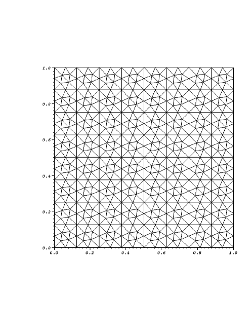
Meshes. The domain is recovered by admissible triangles see figure 2.
Figures 3 - 6 show the diffusive effects of the capillary terms, notably the dissipation of chocs due to the hyperbolic operator Fig. 6. In fact, during the stage of the displacement saturation shock propagate through rock for flows where capillarity terms are neglected, see figure 6. This shock, where capillarity effects are signifiant, it is diffused. However, a part of the the shock wave maintains its sharp front.
 |
 |
 |
 |
 |
 |
 |
 |
References
- [1] H.W. Alt and S. Luckhaus. Quasilinear elliptic-parabolic differential equations. Math. Z., 3, pages 311–341, 1983.
- [2] B. Amaziane and M. El Ossmani. Convergence analysis of an approximation to miscible fluid flows in porous media by combining mixed finite element and finite volume methods. Wiley InterScience (www.interscience.wiley.com). DOI 10.1002/num.2029, 2007.
- [3] Y. Amirat, D. Bates, and A. Ziani. Convergence of a mixed finite element-finite volume scheme for a parabolic-hyperbolic system modeling a compressible miscible flow in porous media. Numer. Math., 2005.
- [4] T. Arbogast. Two-phase incompressible flow in a porous medium with various non homogeneous boundary conditions. IMA Preprint series 606, 1990.
- [5] K. Aziz and A. Settari. Petroleum reservoir simulation. Applied Science Publishers LTD, London, 1979.
- [6] J. Bear. Dynamic of flow in porous media. Dover, 1986.
- [7] M. Bendahmane, Z. Khalil, and M. Saad. Convergence of a finite volume scheme for gas water flow in a multi-dimensional porous media. submitted, 2010.
- [8] Y. Brenier and J. Jaffré. Upstream differencing for multiphase flow in reservoir simulation. SIAM J. Numer. Anal., 28:685–696, 1991.
- [9] F. Caro, B. Saad, and M. Saad. Two-component two-compressible flow in a porous medium. Acta Applicandae Mathematicae (accepted), DOI: 10.1007/s10440-011-9648-0 (2011).
- [10] G. Chavent and J. Jaffr . Mathematical models and finite elements for reservoir simulation: single phase, multiphase, and multicomponent flows through porous media. North Holland, 1986.
- [11] Z. Chen. Degenerate two-phase incompressible flow. existence, uniqueness and regularity of a weak solution. Journal of Differential Equations, 171:203–232, 2001.
- [12] Z. Chen. Degenerate two-phase incompressible flow. regularity, stability and stabilization. Journal of Differential Equations, 186:345–376, 2002.
- [13] Z. Chen and R. E. Ewing. Mathematical analysis for reservoirs models. SIAM J. math. Anal., 30:431–452, 1999.
- [14] L. Evans. Partial Differential Equations. American Mathematical Society, 2010.
- [15] R. Eymard, T. Gallouët, and R. Herbin. Finite Volume Methods, volume 7. Handbook of Numerical Analysis, P. Ciarlet, J. L. Lions, eds, North-Holland, Amsterdam, 2000.
- [16] R. Eymard, R. Herbin, and A. Michel. Mathematical study of a petroleum-engineering scheme. Mathematical Modelling and Numerical Analysis, 37(6):937–972, 2003.
- [17] X. Feng. On existence and uniqueness results for a coupled systems modelling miscible displacement in porous media. J. Math. Anal. Appl., 194(3):883–910, 1995.
- [18] G. Gagneux and M. Madaune-Tort. Analyse mathematique de models non lineaires de l’ingeniere petrolière, volume 22. Springer-Verlag, 1996.
- [19] C. Galusinski and M. Saad. On a degenerate parabolic system for compressible, immiscible, two-phase flows in porous media. Advances in Diff. Eq., 9(11-12):1235–1278, 2004.
- [20] C. Galusinski and M. Saad. A nonlinear degenerate system modeling water-gas in reservoir flows. Discrete and Continuous Dynamical System, 9(2):281–308, 2008.
- [21] C. Galusinski and M. Saad. Two compressible immiscible fluids in porous media. J. Differential Equations, 244:1741–1783, 2008.
- [22] Z. Khalil and M. Saad. Solutions to a model for compressible immiscible two phase flow in porous media. Electronic Journal of Differential Equations, 2010(122):1–33, 2010.
- [23] Z. Khalil and M. Saad. On a fully nonlinear degenerate parabolic system modeling immiscible gas-water displacement in porous media. Nonlinear Analysis, 12:1591–1615, 2011.
- [24] D. Kroener and S. Luckhaus. Flow of oil and water in a porous medium. J. Differential Equations, 55:276–288, 1984.
- [25] S. N. Kruzkov and S. M. Sukorjanskii. Boundary problems for systems of equations of two-phase porous flow type; statement of the problems, questions of solvability, justification of approximate methods. Math. USSR Sb., 33:62–80, 1977.
- [26] A. Michel. A finite volume scheme for the simulation of two-phase incompressible flow in porous media. SIAM J. Numer. Anal., 41:1301–1317, 2003.
- [27] D.W. Peaceman. Fundamentals of Numerical Reservoir Simulation. Elsevier Scientific Publishing, 1977.
- [28] B. Saad. Mod lisation et simulation num rique d’ coulements multi-composants en milieu poreux. Th se de doctorat de l’Ecole Centrale de Nantes, 2011.