Probability Theory
Compatible with the New Conception
of Modern Thermodynamics.
Economics and Crisis of Debts

Abstract

We show that Gödel’s negative results concerning arithmetic, which date back to the 1930s, and the ancient “sand pile” paradox (known also as “sorites paradox”) pose the questions of the use of soft sets and of the effect of a measuring device on the experiment. The consideration of these facts led, in thermodynamics, to a new one-parameter family of ideal gases. In turn, this leads to a new approach to probability theory (including the new notion of independent events). As applied to economics, this gives the correction, based on Friedman’s rule, to Irving Fisher’s “Main Law of Economics” and enables us to consider the theory of debt crisis.

Introduction

The outstanding physicist Ya. I. Frenkel wrote: “We easily get used to the monotonous and unchanging, we stop noticing it. What we are used to seems natural to us, things we are not used to seem unnatural and non-understandable. … Essentially, we are unable to understand, we can only get used to”.

In [1], Henri Poincaré, in particular, writes: “If a physicist finds a contradiction between two theories that are equally dear to him, he will sometimes say: do not worry about this; the intermediate links of the chain may be hidden from us, but we will strongly hold onto its ends” [1, p. 104].

Beginning with the creation of satellites and experiments in the absence of the gravitational field of Earth, a new period in physical experimental investigations of thermodynamical phenomena began. For example, in an equilibrium state, the liquid will have the form of a spherical drop.

It should be noted that previously the relevant experiments were carried out on the surface of the earth, and hence were subjected to gravitational attraction. Therefore, the coagulating drops fell to the ground and the liquid was underneath and the gas above. Coagulation of drops occurs, in particular, because of the Earth’s gravity.

On the other hand, computer-aided experiments have been developed so greatly that a new science arose, the so-called molecular dynamics.

Significant changes also occurred in the mathematical sciences. Therefore, it is not surprising that great progress was also made in such a science as thermodynamics. The difficulty is that everybody is used to the old thermodynamics based on the Boltzmann distribution. Mathematical theorems imply some other distributions, and no contradictions are admissible in mathematics. Therefore, one should not hold on to the end corresponding to the old thermodynamics based on the Boltzmann distribution. As for the Gibbs distribution for the Gibbs ensemble, this distribution can be justified rigorously.

*  *  *

In his 1903 treatise “La science et l’hypothèse,” Henri Poincaré ([1], Chap, 11) closely connects probability theory with problems in thermodynamics. In particular, he writes: “Has probability been defined? Can it even be defined? And if it cannot, how can we venture to reason upon it? The definition, it will be said, is very simple. The probability of an event is the ratio of the number of cases favorable to the event to the total number of possible cases…We are…bound to complete the definition by saying, “ …to the total number of possible cases, provided the cases are equally probable.” So we are compelled to define the probable by the probable. …The conclusion which seems to follow from this is that the calculus of probabilities is a useless science, that the obscure instinct which we call common-sense, and to which we appeal for the legitimization of our conventions, must be distrusted.”  [1, pp. 89–90].

On the other hand, Poincaré speaks of the principles of thermodynamics, the laws of Boyle–Mariotte and Gay–Lussac, and Clausius’ approach to molecular physics. Poincaré writes: “I may also mention the celebrated theory of errors of observation, to which I shall return later; the kinetic theory of gases, a well-known hypothesis wherein each gaseous molecule is supposed to describe an extremely complicated path, but in which, through the effect of great numbers, the mean phenomena which are all eve observe obey the simple laws of Mariotte and Gay–Lussac. All these theories are based upon the laws of great numbers, and the calculus of probabilities would evidently involve them in its ruin.” [1, p. 90].

Certainly, Poincaré gave the standard definition of probability as the ratio of the number of cases favorable for the event to the total number of possible events  and gave a counterexample to this definition of probability. This definition must be completed, writes Poincaré, by the sentence “under the assumption that these cases are equiprobable” ([1, p. 90]) and notes that we have completed a vicious circle place by defining probability via probability.

After this, Poincaré writes: “The conclusion which seems to follow from this  is that the calculus of probabilities is a useless science, that the obscure instinct which we call common sense, and to which we appeal for the legitimization of our conventions, must be distrusted.” ([1, p. 89]).

Thus, the problem is to define first of all what cases are to be regarded as equiprobable in the most natural way. “We are to look for a mathematical thought,” writes Poincaré, “where it remains pure, i.e., in arithmetic” ([1, p. 8]).

Kolmogorov’s definition of elementary events which can be taken for a “complete family of equiprobable events” is based on intuition, i.e., on “the obscure instinct which we call common-sense,” see above. Kolmogorov’s theory, and especially the concept of independent events, well agrees with the Boltzmann distribution. Kolmogorov’s probability theory gave way to a wide spectrum of applications.

A new conception of thermodynamics, which differs from the Boltzmann distribution, must lead to a new conception of probability theory, and especially to a new interpretation of the notion of independent variables.

Thus, Poincaré, a great mathematician, who became the Chairman of the Theory of Probability at the University of Paris (the Sorbonne) at the young age of 32, considers the possibility “that the calculus of probabilities is a useless science” and rejects the idea that “this calculus” is to “be condemned,” in particular, because of thermodynamics (and “the kinetic theory of gases”). Since we have constructed a new thermodynamics, the idea arises to construct a new probability theory corresponding to this thermodynamics in such a way that the notion of independent events would correspond to the new Kolmogorov’s conception, namely, to complexity theory, rather than the old notion corresponding to the Boltzmann distribution.

First of all, in Kolmogorov’s theory, the passage to the limit with respect to the number $N$ of independent tests is of the form

$$p_{i}=\frac{N_{i}}{N},$$

where $N_{i}$ stands for the number of cases favorable for the event, as $N\to\infty$ and $\sum N_{i}=N$. And, if the expectation $M$ of the family $\{\lambda_{i}\}$ is given before the passage to the limit with respect to the number of tests, then we can write

$$MN=\sum\lambda_{i}N_{i},\qquad\sum N_{i}=N.$$ (1)

Denote $MN$ by $M^{\prime}$. Let us take into account that the numbers $M^{\prime}$ and $N$ are large.

Consider the simplest case $\lambda_{i}=i$,

$$M^{\prime}=\sum iN_{i},\qquad\sum N_{i}=N.$$ (2)

I hope there will be no confusion if we shall omit the prime.

Example 1.

In the problem known under the title “partitio numerorum” 2 (see Example 5 below), we may consider all versions of partitioning a number $M$ into $N$ summands as equiprobable events, provided that $N<M$. For example, we may assume that the partitions of the number 5 into the sum 1+4 and into the sum 2+3 are equiprobable.

Here we undertake an essential deviation from the Kolmogorov probability; however, we approach Poincaré’s point of view concerning arithmetic. The question is, what are specific problems to which the new probability theory can be applied?

Kolmogorov [2] writes: “The probability approach is natural in the theory of transmission, over communication channels, of “mass” information consisting of many disconnected or weakly connected messages subjected to certain probability laws. In problems of this kind, the confusion of probabilities and frequencies within the limits of a single sufficiently long time series (this confusion can rigorously be justified under the conjecture of a rather fact mixing), which is deep-rooted in applied researches, is also practically harmless.” …“If there is still some dissatisfaction, it is related to a certain vagueness of our conceptions dealing with relationships between the mathematical probability theory and practical “random phenomena” in general.”

The new probability theory corresponding to the new conception of thermodynamics must adequately describe situations (for example, in computer simulation) with many agents, and also for the case in which the analysis involves “people.” This theory must meet the requirements of semiotics when the number of symbols is very large. This theory must be related to the Zipf law and to similar laws, and also must be applicable to stock exchange speculation (see [3]). As we shall see below, the velocity of money and the occurrence and repayment of debts are also related to problems of new probability theory.

Introduction of an additional parameter $N$ in the probability theory is very essential, although it finally tends to infinity, $N\to\infty$. In particular, it follows from the principle of Lagrange undetermined multipliers that, in the process of calculation of the entropy maximum, the quantities $N$ and $M$ are associated with the following two parameters: the chemical potential $\mu$ and the inverse temperature $\beta=1/T$, where $T$ is the temperature. Thus, the “number of measurements” $N$ is associated with a new parameter $\mu$, which must play a key role in the new probability theory.

1 Gödel’s theory, “sand pile” paradox, and the Bose–Einstein distribution

Albert Einstein remarked towards the end of his career that he only

went to his office at Princeton “just to have the privilege of walking

home with Kurt Gödel.”

“The Forgotten Legacy of Gödel and Einstein ” P. Yourgrau

There is a famous dictum of Kronecker, one of the greatest mathematicians of the 19th century: “The natural numbers are from God, all the rest is the handiwork of man.” In the paper “On the Dogma of the Natural Numbers” [Uspekhi Mat. Nauk, 28 (4), 243–246 (1973), in Russian], P. K. Rashevskii [Rashevsky] wrote: : “The famous negative results of Gödel in the thirties are founded on the belief that, however long you continue the construction of mathematical formulas for a given (totally formalized) mathematical theory, the principles of counting and ordering the formulas remain ordinary, i.e., subjected to the scheme of natural series. Certainly, this belief was not even explicitly stipulated, because it was assumed to be obvious to this very extent.”

Recall that Gödel’s “negative results” (the impossibility of proving the consistency of arithmetic by means of arithmetic or any formal theory containing arithmetic) destroyed the foundation of Hilbert’s program for constructing all of mathematics as a completely formalized system. Indeed, it follows from Gödel’s Incompleteness Theorem that any formal system containing the natural number series (i.e., containing its usual axiomatization) is flawed in principle: if it is consistent, it must be incomplete, since it must contain true arithmetical statements that can neither be formally proved nor disproved. The analysis of the constructions of the great Gödel shows that these arithmetical statements are related, via the principle of mathematical induction, to extremely large numbers. It is well known that Hilbert, after the incompleteness of any noncontradictory formal theory containing arithmetic was proved, fell into a prolonged depression.

The author conjectures that Gödel’s theorem leads to the explanation of several paradoxes of thermodynamics, provided one makes use of an additional instrument, for instance, of a measuring device. Let us present a few elementary examples.

Already in the 4th century B. C., the Greek philosopher Eubulides of Miletus formulated the sandpile paradox: beginning with what number of grains of sand can their collection be regarded as a pile?

First let us comment on this question.

1. When a pile of sand is measured, instead of counting the grains, one ordinarily uses a spoon, or a cup, or some weighting device, and any other arithmetic averaging as well.

2. When such a measurement is performed, precision is lost: the spoons are filled with a number of grains of sand known only approximately, only up to several grains.

The first factor results in the appearance of a new arithmetic for the subsets of the given set of grains, i.e., one more mapping of the subsets of the given set to the set of natural numbers.

The second factor leads to a small loss of precision, to so-called “fluctuations” or, from the mathematical point of view, to “fuzzy sets” or “soft sets.” What fluctuations are admissible?

Consider the simple example of a cup of tea into which we have mixed a spoonful of sugar. We wait for the liquid in the cup to stop rotating, to become calm, but still remain hot. This means that we allow some fluctuation of the liquid; otherwise, it will cool off. The less fluctuations are allowed, the colder the tea will become and the longer we will have to wait before beginning to drink our tea. If the fluctuations are already admissible from our point of view, we say that the tea has been calmed. (This process is quite similar to passing from nonequilibrium thermodynamics to equilibrium thermodynamics, in which only fairly small fluctuations are allowed.)

Already in the second half of the 20th century, mathematicians have attempted to carry out a reform of the natural numbers from the point of view of “fuzzy sets,” “interval analysis,”  “nonstandard analysis,” and the like [4]–[8]; see also [9]. To use the language of physics, this involves taking fluctuations into consideration.

One can modify Kronecker’s statement in the following way: God created air, and therefore created the Avogadro and the Loschmidt numbers, i.e., quantities from $10^{19}$ to $10^{23}$, and also the unavoidable fluctuations of air. This implies the practical impossibility of calculating such quantities exactly.

In his famous work “What is life (from the point of view of physics)?” Schrödinger put forward the hypothesis that if the number of particles $N$ is large enough, then we cannot obtain a calculation result with precision better than $\sqrt{N}$. And Schrödinger called this a “law of nature.” More precisely, in mathematical terms, this can be expressed by saying that the probability of an error in the calculation of $N$ being greater than $\sqrt{N}$ is sufficiently small. We call this a “soft set” of $N$ elements. Schrödinger’s “law of nature” contradicts the dogma (axioms) of the natural numbers.

Thus, first of all, a sandpile is a soft set, with the important properties that (1) it presents another mapping (of its subsets) to the natural numbers and (2) it possesses admissible fluctuations.

Finally, let us pass to the main property of the sandpile, which consists in the following. If we interchange two grains of sand in the pile, then it remains the same pile, i.e., the concept will not change and the rules of its arithmetic will not change.

This means that although the grains of sand are different (they can be distinguished by a scrupulous study), within the sandpile they lose their individuality. And therefore, in the pile they do not obey the Boltzmann statistics, but a statistics of the Bose–Einstein type.

For example, if we buy a pound of sugar, the calculation of the exact number of grains of sugar is not only extremely difficult, but also has no practical meaning. However our “pile” of sugar can be divided into two half kilo piles or into ten piles of 100 grams each. The addition and multiplication for them remain. In other words, for piles the rules of arithmetic still hold. The scale is determined by a macro-measuring device (for example, by a balance with weights; we assume for the sake of simplicity of our presentation that there is also a minimal weight).

Let us repeat once again: if, under the interchange of two grains, the notion of pile does not change, and neither do the rules of arithmetic for piles, then the individuality of particles of sand within the pile are lost. This is the main property of piles. From the point of view of statistical physics, this corresponds to passing from Boltzmann statistics (from the Boltzmann entropy, which is equal to the Shannon entropy) to a one-parameter family of statistics of the Bose–Einstein type, although grains of sand can be distinguished from each other and there are no identical grains.

Example 2.

Let us put two one-copeck coins in two banks and calculate the number of possible variants of this decomposition.

(1) We put two coins in the first bank and nothing in the second one.

(2) We put two coins in the second bank and nothing in the first one.

(3) We put per one coin in each bank.

Thus, we have three variants. This is the Bose-type statistics.

Now we calculate the number of possible variants of putting a one-copeck coin and a one-pence coin in two banks. In this case, variant (3) splits into the following two variants: we put the copeck in the first bank and the pence in the second bank or we put the pence in the first bank and the copeck in the second bank. As a result, we have four possible variants. This is the Boltzmann statistics.

Similarly, the decomposition of $M$ copeck coins over $N$ banks gives the Bose-type statistics. If you put a 1000-rouble bond on your bank account and then want to take it back, it is hardly probable that you obtain the same 1000-rouble bond (with the same number).

Quite similarly, the conveyance of $M$ loaves of bread from a big baker’s shop over $N$ bakeries satisfies the Bose-type statistics. But the variety of proposed loaves, the purchaser in a bakery can choose a certain loaf that he likes most of all. These situations are determined by the words ”wholesale” (i.e. vegetables and fruit are measured in containers, e.g. in barrels with volume $V_{\delta}$) and “at retail”.

This is an example of the “sandpile” paradox: while the set of elements is treated as a pile, its elements are subjectively indistinguishable and satisfy the Bose-type statistics. In our case, it is meaningful to distinguish the elements of the set, then this is already not a pile, and it satisfies the Boltzmann statistics.

If we consider a set of grains before the formation of a pile (i.e., before the time moment at which the set can be measured by a macroscopic device), then the transposition of grains gives another natural series as compared with the original one. If we continue extending the new natural number series according to Boltzmann, the difference between the statistics will disappear. This is similar to the one-parameter family of hyperbolic geometries whose curvature vanishes as they become Euclidean.

Let us cover the actual (practical) natural series  by a system of soft subsets of $N$ elements, which meet one another in the domain of fluctuations in general. It is assumed that the union of these subsets contains the entire natural series and that $N>10^{6}$. The union of pairs of subsets of $2N$ elements contains the natural series again and, continuing the process of adding a new pile, $3N$, $4N$, …, we obtain an arithmetic of soft subsets and a practical natural series of piles.

We would like to say in advance that equilibrium thermodynamics is related to these very deep logical problems.

If we supplement the dogma of the natural numbers with an external measuring device without denying the commutativity of addition, this will not contradict the fact that we are counting only up to some precision, and if probability is taken into consideration, will allow counting up to some given “soft” precision. This soft precision allows to count all the elements of a finite set. We are only saying that if this unprecise count differs from the exact one, then we can disregard the error. The so-called equal distribution law only concerns small natural numbers. This law must also be modified. And this contradicts our habitual philosophy, accepted for centuries, and can therefore generate protests not only from scientists, but also from philosophers.

Progressive Russian men of letters, for example, Chernyshevskii, categorically refused to accept Lobachevsky’s geometry.

Note that Lobachevskian geometry is in fact a one-parameter family of geometries, depending on the radius (curvature), which passes to Euclidean geometry as the radius tends to infinity.

Soviet philosophers ostracized the followers of Bohr’s Complementarity Principle, which he borrowed from biology and psychology. At the same time, if we accept this complementarity principle as a “complement” to the new concept of the number $N$ of particles with admissible fluctuations of $\sqrt{N}$, then we come to the notion of chemical potential $\mu$ and to an assertion similar to Heisenberg’s Indeterminacy Principle: the smaller the fluctuations of $\mu$, the smaller the fluctuations of $N$. And, further, we come to other intensive and extensive quantities that characterize thermodynamics.

First of all, the pressure $P$ exercised by the piston decreases the volume $V$ of air in the vessel, and Bohr’s Complementarity Principle relates these two substances. The increase of the temperature $T$ increases the chaotic speed of particles, it increases the chaos determined by the entropy. These two quantities correspond by Bohr’s Complementarity Principle.

Bohr’s Complementarity Principle is related to Heisenberg’s Indeterminacy Principle, namely, the decrease in the fluctuation of one component corresponds to an increase of the complementary quantity. Bohr explains this principle by the interference of the measuring device. In our example with sugar, the macro-measuring device (the balance) also plays its role. Especially if, in the weighting process, “self-feeding” processes occur, similar to to those taking place when temperature is measured by a mercury thermometer, which “absorbs into itself” part of the energy (heat) of the particles that it is supposed to measure.

Bohr’s Complementarity Principle was developed and applied not only by physicists with a wide outlook such as Max Born, but also by such pragmatists as Pauli. According to the Complementarity Principle, motion and immobility, for example, were compared. But a special role is played by the Complementarity Principle in equilibrium or nonequilibrium thermodynamics.

Just as the existing “time-energy” complementarity, in thermodynamics there is the complementarity “observation time – size of the fluctuation,” since we come to a situation of equilibrium thermodynamics, as we explained in the cup of tea example. Here an essential role is played by viscosity, the slowing down phenomenon that leads to equilibrium thermodynamics up to a concrete value of the fluctuation. The old thermodynamics was based on the Boltzmann statistics, and the latter on the dogma of natural numbers. But it turned out that the dogma of natural numbers is just as unfit for very large collections considered in thermodynamics as Euclidean geometry is for the description of the Universe.

Below we construct a one-parameter family of ideal gases that describe such very large collections.

Example 3.

As an example of the famous Erdős theorem from number theory, we consider the solution of the ancient problem partitio numerorum. This problem features an integer $M$, which is expanded into $N$ summands; for example, suppose that $M=5$ and $N=2$:

$$5=1+4=2+3;$$

this yields $\mathcal{M}=2$ variants of the solution of this problem.

If $M=10^{23}$ and $N=1$, then there is only one variant of the expansion: $\mathcal{M}=1$. If $M=10^{23}$ and $N=10^{23}$, then there is also only one variant of the expansion: the sum of 1’s, i.e., $\mathcal{M}=1$.

Obviously, for a fixed number $M$, there exists a number $N_{c}$ for which the number of variants $\mathcal{M}$ of the expansion is a maximum (in general, this number is not unique). The quantity $\log_{2}\mathcal{M}$ is called Hartley’s entropy. At the point where it attains its maximum, one has the maximum of the entropy. The chemical potential equal to zero corresponds to this point.

Suppose we are given the partition

$$M=a_{1}+\dotsb+a_{N}$$

of the number $M$ into $N$ summands. Let $N_{j}$ be the number of summands on the right-hand side of this equation that are precisely equal to the number $j$.

Then there are $\sum_{j}N_{j}$ in all, and this number is equal to $N$, because we know that there are only $N$ summands. Further, the sum of summands equal to $j$ is $jN_{j}$, because their number is $N_{j}$; hence the sum of all summands is obtained by summing these expressions over $j$, i.e., $\sum_{j}jN_{j}$, and it is $M$. Namely,

$$\sum_{0}^{\infty}N_{i}=N,\qquad\sum_{0}^{\infty}iN_{i}=M.$$ (3)

The nonuniqueness of this maximum and the indeterminacy of the number of these maxima allowed Erdős to obtain his result only up to $o(\sqrt{M})$. Thus, he retreated from the dogma of the natural numbers in the direction of the notion of soft set.

Relations 3 correspond to physical relations of the form

$$\sum^{\infty}_{i=0}N_{i}=N,\qquad\sum^{\infty}_{i=0}\varepsilon_{i}N_{i}={\mathcal{E}},$$ (4)

where $N_{i}$ is the number of particles at the $i$th energy level, the $\varepsilon_{i}$ are the discrete collections of energies, and $\mathcal{E}$ is the energy.

The derivation for the general case, which coincides for $E=p^{2}/2m$ (where $p$ stands for the momentum and $m$ for the mass of the particle), coincides with the Bose distribution presented for the volume $V=1$ by Landau and Lifshits in [11], is considered in [12--14].

1.1 One-Parameter Family of Distributions of the “Partitio Numerorum” Type

Let us briefly present results of the papers listed above.

If we consider the particular nonrelativistic case in which the Hamiltonian $H$ of the system is ${p^{2}}/{2m}$, where $p$ is the momentum and $m$ the mass, then, up to constant multipliers, problem 3 corresponds to the two-dimensional case.

Consider a straight line and a plane. Let us mark off the points $i=0,1,2,\dots$ on the straight line and the points $x=i=0,1,2,\dots$ and $y=j=0,1,2,\dots$ on the coordinate axes $x,y$ of the plane. With this set of points $(i,j)$ we associate the points on the line, which constitute the sequence of natural numbers $l=1,2\dots$. To each point let us assign the pair of points $i$ and $j$ by the rule $i+j=l$. The number of such points $n_{l}$ is $l+1$. This is the two-dimensional case.

Consider the three-dimensional case. On the axis, set $z=k=0,1,2,\dots$, i.e., set $i+j+k=l$. In this case, the number of points $n_{l}$ is

$$n_{l}=\frac{(l+1)(l+2)}{2}.$$

For the $D$-dimensional case, it is easy to verify that the sequence of weights (multiplicities) of the number of variants

$$i=\sum_{k=1}^{D}m_{k}$$,

where the $m_{k}$ are arbitrary natural numbers, is of the form:

$$q_{i}(D)=\frac{(i+D-2)!}{(i-1)!(D-1)!}.$$ (5)

The three-dimensional case $D=3$ corresponds to the following problem of number theory (see [11]):

$$\sum N_{i}=N,\qquad\varepsilon\sum\frac{(i+2)!}{i!6}N_{i}={\mathcal{E}},\qquad\frac{\mathcal{E}}{\varepsilon}=M.$$ (6)

As was already stated, Schrödinger thought that the statistical laws valid as $N\to\infty$, where $N$ is the number of particles, hold with accuracy at most up to $\sqrt{N}$.

However, such a rough estimate also has a positive aspect.

This consideration enables us to extend the number theory presented above no noninteger dimensions.

Let us consider expressions of the form

$$\varepsilon\sum\frac{\Gamma(d+i)}{\Gamma(i+1)\Gamma(d+1)}N_{i}\leq{\mathcal{E}},$$ (7)

$$\sum N_{i}=N,$$ (8)

where $d=D/2$ and $\Gamma(d)$ is the gamma function.

Let $\mathcal{M}$ be the number of solutions satisfying inequality 7 and relation 8 for a noninteger $D$ (the “fractal dimension”).

Let us define the constants: the chemical potential $\mu$ and the inverse temperature $\beta=1/T$ “conjugate”  to $N$ and ${\mathcal{E}}$.

Consider the three-dimensional case. We have

$$N=\sum^{\infty}_{i=1}\frac{(i+1)(i+2)}{2(e^{\beta(i-\mu)}-1)}=\sum N_{i},$$ (9)

$$M=\frac{\mathcal{E}}{\varepsilon}=\sum^{\infty}_{i=1}\frac{i(i+1)(i+2)}{2(e^{\beta(i-\mu)}-1)}.$$ (10)

This is a well-known result in number theory [12]–[14]. It is very simple as compared with the Erdös theorem.

Here we have used the fact that arithmetic summands can be rearranged and have summed the elements of the “pile” over all rearrangements each corresponding to a particular sequence of natural numbers. According to Boltzmann, each rearrangement yields a new pile, but, for us, it is one pile. Thus, we carry out a procedure similar to that used by Landau and Lifshits in their calculation of the Bose–Einstein distribution.

Now the distribution takes the form of the Bose–Einstein distribution [11] in which $V=1$.

In the general case, for $D>2$,

$${\mathcal{E}}=\varepsilon\sum^{\infty}_{i=1}\frac{iq_{i}}{e^{\beta(i-\mu)}-1},$$ (11)

where

$$q_{i}=\frac{\Gamma(i+d)}{\Gamma(d)\Gamma(i+1)},\qquad N=\sum^{\infty}_{i=1}\frac{q_{i}}{e^{\beta(i-\mu)}-1}.$$ (12)

Since, for a fixed $k$, the number of particles $N$ tends to infinity, we can pass from sums to integrals by the Euler–Maclaurin estimates and obtain the following relation.

Landau and Lifshits [11] write: “Any macroscopic state of an ideal gas can be characterized as follows. Let us distribute all the quantum states of an isolated particle of the gas over groups each of which contains close states (possessing, in particular, close energies); further, the number of states in each group and the number of particles contained in them is very large. Renumber these groups of states by $j=1,2,\dots\,$, and suppose that $G_{j}$ is the number of states in the $j$th group, while $N_{j}$ is the number of particles in these states. Then the collection of numbers $N_{j}$ will fully characterize the macroscopic state of the gas” [11, Russian, p. 143].

The “groups,” which are also called “cells,” contain the quantum eigenvalues (states). The number of these states in each cell can be roughly associated with the quantum spectrum density and corresponds to the fractal dimension.

Therefore, without regard for the interaction, we obtain a macro parameter defining the spectrum density $\widetilde{Z}=\mathcal{E}/NT$ of a given molecule. We can state that this quantity $\widetilde{Z}$ is the macro measurement of the whole quantum spectrum density of a given molecule for the case of the maximal $\mathcal{M}$, i.e. for the chemical potential $\mu=0$.

Landau and Lifshits make the following remark concerning the “momentum space:” “The phenomenon of accumulation of particles at the state with $\varepsilon_{i}$, $i=0$ is often referred to as the “Bose–Einstein condensation.” We stress that one can speak here only about the “condensation in the momentum space;” certainly $(!)$, there is no practical condensation in the gas” [11]. However, we claim that a practical condensation in an ordinary gas occurs indeed under certain conditions, see Section 2.

The energy $\mathcal{E}$ (which, when divided by $\varepsilon$, is equal to the original number $M$ in the problem of partitio numerorum) for $\gamma=(d-1)/2$, where $d$ stands for the “fractal” noninteger dimension, $d=D/2$, is of the form

$$\mathcal{E}=\frac{T^{2+\gamma}}{\Lambda^{2(1+\gamma)}\Gamma(2+\gamma)}\int_{0}^{\infty}\xi^{1+\gamma}\bigg{\{}\frac{1}{e^{(\xi-\kappa)}-1}\bigg{\}}\,d\xi=\frac{1}{\Lambda^{2(1+\gamma)}}T^{2+\gamma}\operatorname{Li}_{\gamma+2}(e^{\mu/T}),\qquad\kappa=\frac{\mu}{T},$$ (13)

where $\operatorname{Li}_{\gamma}(\cdot)$ is the polylogarithm, $\operatorname{Li}_{\gamma+2}(1)=\zeta(\gamma+2)$, e.g., for $\mu=0$, $\zeta$ is the Riemann zeta function, and $\Lambda$ is a constant. 

Now we can rigorously mathematically formulate the main principle of thermodynamics corresponding to the approximate conservation of the gas density (this corresponds to the physicists’ statement in equilibrium thermodynamics: “the density is homogeneous in a vessel;” physicists consider equilibrium thermodynamics as a separate discipline, after which fluctuation theory is also considered separately).

The experimenter assumes that the density of particles inside the vessel is constant up to fluctuations (of the order of the root of the number of particles inside a small subvolume). This means that he counts the number of particles in each small subvolume in which there are at least one million particles and the density is approximately constant. In each fixed subvolume $V$, there is the same fuzzy number of particles $N_{\delta}$. Obviously, any rearrangement of the numbers of particles does not affect their density (just as in arithmetic, a rearrangement of summands does not affect their sum). If we even assume that the experimenter numbered all the particles in the previous measurement, then, in the next measurement, e.g., after increasing the pressure inside the vessel by using a piston and after achieving the equilibrium (i.e., the homogeneity of the density in the vessel), he cannot state what number corresponds to a particular particle and, therefore, must again number all the particles to find their density. This is a fact of arithmetic, and arithmetic is the foundation of analytic number theory.

1.2 The Main Principle of Equilibrium Thermodynamics (Uniform Density) and the Family of Ideal Gases Corresponding to Every Molecule

First, let us roughly state this principle: the density (more precisely, concentration) of a gas in a closed vessel is almost constant and almost equal to the number of particles in the vessel divided by the volume of the vessel.

This principle can be stated in a mathematically rigorous way as follows.

We consider molecules of one type, i.e., of the same spectrum density. As was already shown, the spectrum density is characterized by the parameter $\gamma$. Assume that the spectrum density of the molecules of this type corresponds to the parameter $\gamma=\gamma_{0}$.

Consider a vessel of volume $V$ containing $N>10^{19}$ identical molecules corresponding to the parameter $\gamma=\gamma_{0}$. Consider a small convex volume of size $V_{\delta}$ containing $N_{\delta}$ particles, where $N_{\delta}$ is not less than $10^{6}$. Let $\mathbb{P}$ be the probability of the event consisting in the deviation of $N_{\delta}$ by a value exceeding $\sqrt{N_{\delta}}$ for any volume of size $V_{\delta}$ inside the vessel. The main principle is that the probability $\mathbb{P}$ is sufficiently small.

Remark 1.

This obvious fact strictly implies a new relation for the ideal gas, separate for each molecule of a pure gas. This is a consequence of a sufficiently simple theorem of number theory.

Remark 2.

The ratio $M/{kNT}$ is “dimensionless” (owing to the Boltzmann constant $k$) in the sense that, in physics, $M$ corresponds to the energy $\mathcal{E}$. The quantity $Z={\mathcal{E}}/{\mathcal{R}T}$, where $\mathcal{R}$ is the gas constant, is called the compressibility factor.

It follows from this principle that the numbering of the particles in a subvolume $V_{\delta}$ is arbitrary, and the concentration (density) is independent of it. We can rearrange the numbers, which does not lead to any change in density: a rearrangement of summands does not affect their sum. Combining this with 13, we prove the following statement.

Corollary 1.

At $\mu=0$, the maximum of $\mathcal{M}$ and the entropy is attained. We obtain a one-parameter family (with parameter $\gamma$) of maximum values of critical compressibility factors

$$Z_{\mathrm{degen}}=\frac{M}{kNT}\bigg{|}_{\mu=0}=\frac{\zeta(\gamma+2)}{\zeta(\gamma+1)}.$$ (14)

What happens with a pure gas for $T<T_{\mathrm{degen}}$? We refer relation 13 for any $\gamma$ as the “Bose gas,” always using the inverted commas in this case.

We see that the formulas obtained above coincide for $\gamma=3/2$ with the formulas for the Bose gas. Landau and Lifshits especially warn in the quatation given above that one must not confuse the Bose condensate with a practical condensate. However, we should ask: Where are the excessive particles when the temperature became lower the “degeneration temperature” for the pure gas for which we have rigorously developed the above formulas 13 from the main postulate? Despite the rigid taboo claimed by Landau and Lifshits (see above), it is natural to assume that the excessive particles had condensed into the liquid phase.

We shall prove this rigorously in the second section for the Wiener quantization of thermodynamics. For now, we present a comparison of experimental graphs with graphs constructed according to our computations and for diverse pure gases in the paper by Apfel’baum and Vorob’ev “Correspondence between of the ideal Bose gas in a space of fractional dimension and a dense nonideal gas according to Maslov scheme” [18].

Thus, we assume that the critical value of the compressibility factor $Z_{\mathrm{c}}$ for the given gas is of the form

$$Z_{\mathrm{c}}=\frac{\mathcal{E}_{\mathrm{c}}}{{\mathcal{R}}T_{\mathrm{c}}}=\frac{\zeta(\gamma+2)}{\zeta(\gamma+1)},\qquad\mathcal{E}_{\mathrm{c}}=P_{\mathrm{c}}V_{\mathrm{c}}.$$ (15)

Hence we obtain the parameter $\gamma$ characterizing the spectrum (“spectral density”) of a given molecule.

Let us compare the critical isotherms on the $V,P$ plane up to the critical point (at which the density is sufficiently high and the pressure is 3–4 times greater than that of the “ordinary” Boltzmann ideal gas).

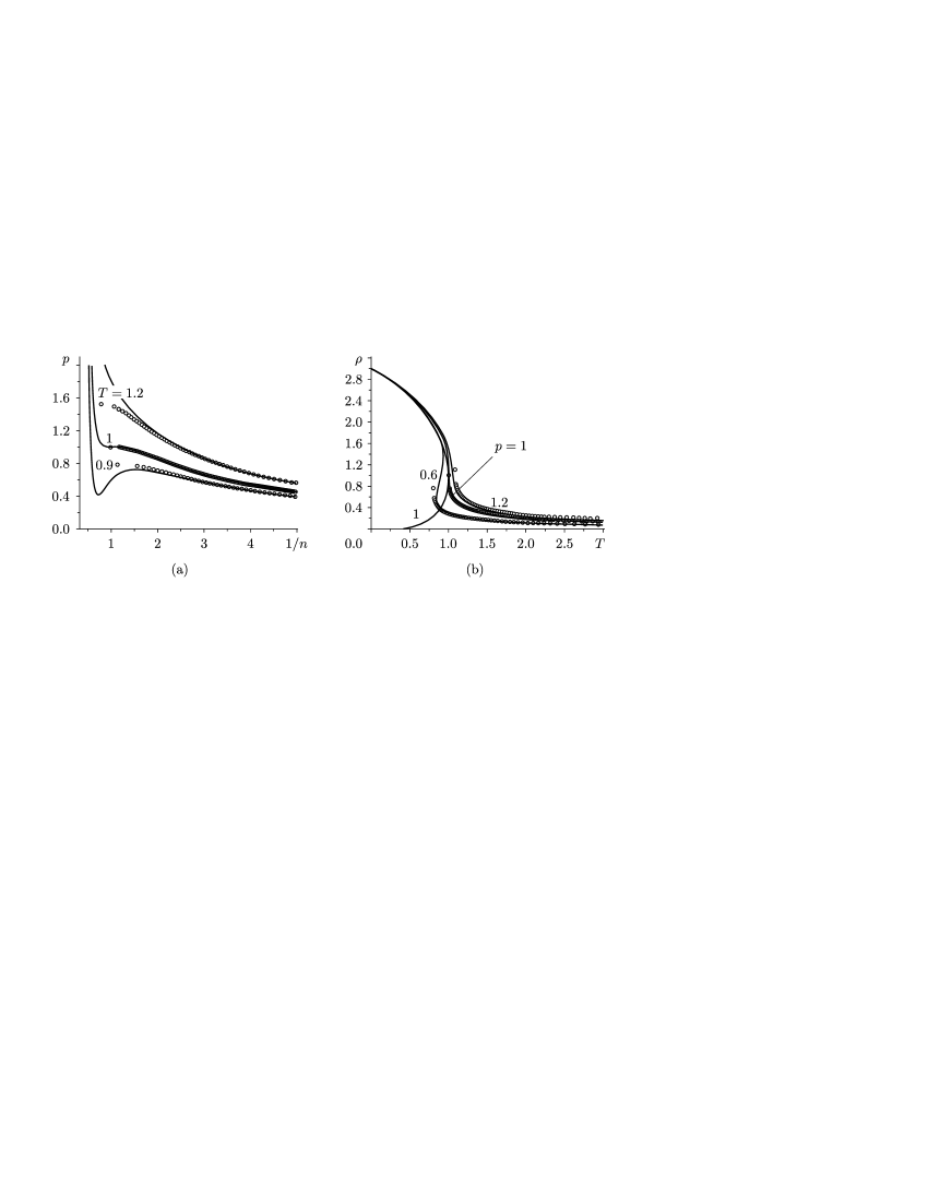
Figure 1: (a) Isotherms of pressure for the van der Waals equation are shown by continuous lines. The small circles show the corresponding lines computed with $\gamma=0.312$ for $\varphi(V)=V$ (i.e., the ideal “Bose gas”), $Z_{\text{cr}}=3/8$, $p=P/P_{\text{c}}$, and $n=N/N_{\text{c}}$.  (b) Isobars of density for the van der Waals equation are shown by continuous lines. Line 1 is the binodal curve. The small circles correspond to isobars for the “Bose gas” with $\gamma=0.312$.

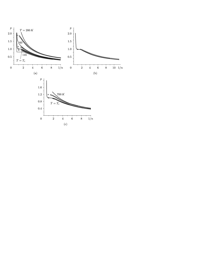
Figure 2: a) Isotherms for argon. The continuous lines correspond to the experimental data, and the line formed by small circles is constructed according to the isotherm of ideal “Bose gas,” $Z_{\text{cr}}=\frac{\zeta(\gamma+2)}{\zeta(\gamma+1)}=0.29$, $p=P/P_{\text{c}}$, and $n=N/N_{\text{c}}$. (b) The same for water, $Z_{\text{cr}}=0.23$. (c) The same for copper, $Z_{\text{cr}}=0.39$.

The approach which takes into account the possibility to preserve the pile under the transposition of two grains fundamentally solves the Gibbs paradox. Note that, although the greatest mathematicians, including von Neumann and Poincaré, tried to patch up the Gibbs paradox, they did not succeed. In the same way, many great physicists tried to clarify the problem with the paradox, and still, all the time, rather serious works occur that try to coordinate with the Gibbs paradox. Last year, ten papers concerning the topic were presented to arXiv.org.

V. V. Kozlov [19] rigorously proved the existence of an entropy jump in the Poincaré model for gas in a parallelepiped with mirror walls, i.e., he establishes the presence of the paradox in this model. The rigorous mathematical work [19] helped to find the solution suggested by the author of the present paper for the Gibbs paradox.

1.3 On the table of molecules versus the energy-spectrum density

The question is how to calculate the average density of the spectrum of a molecule at a given temperature. We consider the energy $\mathcal{E}$ corresponding to $N$ particles in the maximum chaos situation where the number of possible variants of the system solution is maximal, i.e., at the entropy maximum (in the case of maximum indeterminacy). The quantity $\mathcal{E}$ is divisible by $N$; this is the average energy of a single particle. Dividing this average energy by the energy $kT$, we obtain the quantity of energy of a particle per unit energy corresponding to the given temperature: $Z=\frac{\mathcal{E}}{NkT}$. In what follows, we omit the Boltzmann constant, which cannot lead to misunderstanding, because this only means that the temperature is measured in energy units.

We note that a similar construction is developed on the basis of the Boltzmann distribution in Sec. 40 in [11], which is called “Nonequilibrium perfect gas”.

In our case, the quantity $\mathcal{E}/NT$ depends on the dimension $\gamma$ in the space of momenta (or energies $E=\frac{p^{2}}{2m}$, $dE=\frac{p\,dp}{m}$) and hence is a one-parameter family (depending on the parameter $\gamma$, which is the Hausdorf dimension, fractional or fractal dimension).

We obtain a table arranged not according to masses as the Mendeleev periodic table but according to the average energy density. This table comprises all known molecules. The molecule internal energy can be represented as $PV$. The extreme point at the maximal entropy corresponds to the catastrophe in the sense of Arnold. This is (because of the pile basic property) the degeneracy point corresponding to the degeneracy point of the Bose gas in the fractal (fractional) dimension.

Here we do not force the parameter $\gamma$ to fit the experiment. To say that the parameter $\gamma$ is adjusted to experiments is the same as to say that the Mendeleev periodic table is forced to fit the experiment with respect to the mass parameter.

In addition, I note that the maximum entropy point (the point $\mu=0$) corresponds to the focal point (or to the point of catastrophe, as it was called by Arnold) similar to the focus of a lens focusing the Sun rays.

We answer the above question as follows. The mathematicians have been using the dogma of the natural numbers for a very long time. Gödel disproved it only in 1930, and we have already described the state to which the greatest mathematician Hilbert was brought by this proof. Boltzmann died much earlier. He committed suicide, and it was said that precisely the claims of mathematicians underly his deed. As is known, in a very hot discussion with mathematicians about molecules, he shouted: “Go and verify them!”. If he were alive in the after-Gödel times, he would cry to the mathematicians: “Go and number them!”. And the mathematicians who were acquainted with Gödel’s work could not say anything against this.

2 Bohr’s Complementarity Principle, Wiener’s quantization of thermodynamics, and a jump of critical exponents

The equilibrium thermodynamics must follows from the nonequilibrium thermodynamics in the limit as the viscosity tends to zero. In this chapter, we first introduce the notion of viscosity $\nu$ and then let it tend to zero. We introduce the viscosity in “almost” the same way as in hydrodynamics, treating such an approach as the Wiener quantization. In this chapter, we actually consider the limit as $\nu\to 0$.

Balescu wrote: “The Maxwell construction does not provide a molecular explanation of the phase transition below $T_{\mathrm{c}}$: it is merely an ad hoc trick that works, provided we accept a priori the existence of a coexistence region.” [20, p. 305].

Meanwhile, the problem involving the so-called Maxwell rule for the transition “gas–liquid,” which is a natural complement of the new concept (of phenomenological thermodynamics) constructed above, is solved, as was described in detail in [16], by using the tunnel (or Wiener) quantization introduced by the author already in his 1994 works; see [21, 22] and also [23]–[25]. We repeat here this quantization at a heuristic level.

We can say that the quantization of thermodynamics is simply called for. We have already mentioned Bohr’s Complementarity Principle in the previous section. Indeed, we have the phase space  in which the momenta are the extensive quantities $V$ and $-S$, and the corresponding coordinates are $P$ and $T$. The usual quantization is of the form

$$\widehat{V}=ih\frac{\partial}{\partial P},\qquad-\widehat{S}=ih\frac{\partial}{\partial T}.$$ (16)

Just as in [26], let us invoke an analogy between the Schrödinger equation and the heat equation.

A. The Schrödinger equation corresponding to a noninteracting particle without an external field is

$$-ih\frac{\partial\psi}{\partial t}=(ih\nabla)^{2}\psi.$$ (17)

The change of variables

$$\psi=e^{\frac{i}{h}\mathbb{S}}$$

leads to the equation

$$\frac{\partial\mathbb{S}}{\partial t}+(\nabla\mathbb{S})^{2}+ih\Delta\mathbb{S}=0.$$

In this case, the quantization of the classical Hamilton–Jacobi equation consists in the addition of the term $ih\Delta\mathbb{S}$.

B. The heat equation is

$$-\nu\frac{\partial u}{\partial t}=(\nu\nabla)^{2}u,$$ (18)

where $\nu$ stands for the kinematic viscosity. The change of variables

$$u=e^{-\frac{\mathbb{S}}{\nu}}$$

leads to the equation

$$\frac{\partial\mathbb{S}}{\partial t}+(\nabla\mathbb{S})^{2}+\nu\Delta\mathbb{S}=0.$$ (19)

The derivatives of this equation with respect to the coordinates are called the Burgers equations. In this case, the Wiener quantization consists in the addition of the viscous term.

Remark 3.

In this special case, the Wiener quantization coincides with the Euclidean quantization well known in field theory. In the general case, this quantization corresponds to the passage from the Feynman path integral to the Wiener path integral and is in essence presented in detail for physicists in the book [27] by Feynman and Hibbs.

In the Burgers equation, for $p=\partial\mathbb{S}/\partial x$, a shock wave occurs as $\nu\to 0$, i.e., a discontinuity of the $\theta$-function type, whereas, in thermodynamics, we have a jump of the $\theta$-function type for the transition “gas–liquid.” For the Burgers equation, the rule of “equal areas” arises. For the “gas–liquid” transition, the Maxwell rule of equal areas arises. In the heat equation, the tunnel quantization of energy is given by the Heaviside operator $D_{t}=\frac{\partial}{\partial t}$ multiplied by the viscosity, $\widehat{D}_{t}=\nu\frac{\partial}{\partial t}$. In thermodynamics, the thermodynamical potential, the Gibbs energy, is equal to $\mu N$, where $\mu$ stands for the chemical potential and $N$ for the conjugate extensive quantity, the number of particles. Hence, $\widehat{N}=\nu\frac{\partial}{\partial\mu}$, and the role of time  is played by $\log-\mu$, because, under this quantization, the operator $\nu\mu(\partial/{\partial\mu})$ corresponds to the Gibbs energy.

For us, the one-dimensional case $p_{1}=V$ and $q_{1}=P$ is of importance. In the general case, the focal point (the point of inflection [29, 30]) is of the form $q\sim p^{3}$, i.e.,

$$P_{\mathrm{cr}}\sim(V-V_{\mathrm{cr}})^{3}=\bigg{(}\frac{\rho_{\mathrm{cr}}-\rho}{\rho\rho_{\mathrm{cr}}}R\bigg{)}^{3},$$ (20)

which corresponds to the classical critical index (the exponent) equal to three. The asymptotic solution (as $\nu\to 0$) of 19 corresponding to this point is expressed by the Weber function.

Therefore,

$$u(x)=\frac{1}{\sqrt{\nu}}\int_{0}^{\infty}e^{-\frac{px+\widetilde{S}(p)}{\nu}}\,dp,\qquad\lim_{p\to 0}\frac{\widetilde{S}(p)}{p^{4}}<\infty,\qquad\widetilde{S}^{(4)}(p)|_{p=0}\neq 0.$$ (21)

The solution $p_{\nu}(x)$ of the Burgers equation can be evaluated by the formula

$$p_{\nu}(x)=\nu\frac{\partial\log u(x)}{\partial x}=\frac{\int_{0}^{\infty}\exp\{\frac{-x\xi+\widetilde{S}(\xi)}{\nu}\}\xi\,d\xi}{\int_{0}^{\infty}\exp\{\frac{-x\xi+\widetilde{S}(\xi)}{\nu}\}d\xi}.$$ (22)

After the substitution

$$\frac{\xi}{\root 4 \of{\nu}}=y,$$

as $x\to 0$ we obtain

$$p_{\nu}(x)\to_{x\to 0}{\root 4 \of{\nu}}\cdot\text{const}.$$ (23)

In our case, the momentum $p_{\nu}(x)$ is the volume $V$.

If the solution of the relation

$$x=\frac{\partial\widetilde{S}}{\partial p}$$ (24)

is nondegenerate, i.e.,

$$\frac{\partial^{2}\widetilde{S}}{\partial p^{2}}\neq 0$$

at the point

$$\frac{\partial\widetilde{S}}{\partial p}=x,$$

then, in this case, the reduced integral 22 is bounded as $\nu\to 0$. For this integral to have a singularity of order $\nu^{1/4}$, we must apply to this integral the fractional derivative $D^{-1/4}$ with respect to $x$. The value of $D^{-1/4}$ at the function equal to one, $D^{-1/4}1$, gives approximately $x^{1/4}$.

In our case, the pressure $P$ plays the role of $x$, and the volume $V$ plays the role of momentum $p$. Therefore, $V\sim P^{1/4},$ i.e.,

$$P_{\mathrm{cr}}\sim(V-V_{\mathrm{cr}})^{4}\sim\Big{(}\frac{\rho-\rho_{\mathrm{cr}}}{\rho\rho_{\mathrm{cr}}}R\Big{)}^{4}.$$ (25)

Following Green [32], D. Yu. Ivanov, a deep experimenter, poses the following question: Why the deviations from the classical theory in the critical opalescence are observed within the limits of hundredths of a degree from the critical points, whereas the deviations in thermodynamical properties show [33] a nonclassical behavior at a much larger distance from the critical point? Professor Ivanov claims that rather many questions of this kind have accumulated (see, for example, [34]), and all these questions mainly deal with the behavior of practical systems. The point is that, from the point of view of the developed theory of critical indices [35], there must be a drastic passage to the classical indices outside a neighborhood of the critical point.

To make Ivanov’s question understandable for persons who are not experts in critical points, we paraphrase the question for the case of geometric optics, when the sun rays are collected by a magnifying glass to a focus. If we were created a special construction for the vicinity of the focus in which the paper smoulders, then the experimenter could ask why the experiment gives a smooth picture of transition in the double logarithmic coordinates and the indices are preserved far away from the smouldering small vicinity of the focus. In the present case, the smouldering paper can be compared with the small area of opalescence (drastic fluctuations near the critical point) for which a separate theory was constructed. At the same time, the special function defining the point in wave theory (like the Weber function) can be continued quite smoothly to a much wider domain in which the paper does not smoulder. In the opinion of Ivanov, this fact is much more important than the fact that Wilson’s theory gives the index 4.82 rather than 4.3, whereas the latter is given by modern experiments.

Can the experimental index 4.3 be explained in principle in the framework of the conception presented by the author?

Whereas, in classical mechanics, there is no dependence on the Planck constant $\hbar$, in classical thermodynamics we face a slow dependence of the viscosity on $T$ and $\rho$, and thus vice versa as well. In our picture, the “stretching” of $P_{\mathrm{cr}}$ and $T_{\mathrm{cr}}$ in the experiment for real gases (Figs. 10 and 11) is greater than in the van der Waals model, which enables us to introduce the parameter $\nu^{\varepsilon}$ for the “stretching” (i.e., $P=\nu^{\varepsilon}V^{3}$) and obtain the index $\delta=4.3$ for $\varepsilon=0.07$. Thus, in principle, the answer can be “yes.”

It follows from what was said above that new critical indices arise only due to quantization of the conjugate pairs $\{P,V\}$ and $\{T,S\}$. Thus, the relationships between intensive quantities can be taken classical, because everything is carried out under the assumption of infinitely small viscosity. In this case, one can also pass to other coordinates, to the pressure and density. Write, as usual,

$$p=\frac{P-P_{\mathrm{cr}}}{P_{\mathrm{cr}}},\qquad\theta=\frac{T-T_{\mathrm{cr}}}{T_{\mathrm{cr}}},\qquad v=\frac{\rho-\rho_{\mathrm{cr}}}{\rho_{\mathrm{cr}}}.$$

In the classical case, we have ([20, p. 344])

$$p\sim v^{3},\qquad v\sim\theta^{1/2},\qquad\theta\sim v^{2}.$$

In the classical case,

$$p\sim\theta^{3/2}.$$

In the tunnel quantum case, we obtain $\beta=0.375$ (cf. [20, p. 356]) in the limit as $\nu\to 0$, and thus not precisely (the stretching is not taken into account). This is obtained for the van der Waals model quantized in the tunnel way.

If $\nu>0$, then an uncertainty principle arises. Let us proceed to the consideration of this principle.

Thus, for the Wiener quantization, one takes for the main operators the Heaviside operator $\widehat{D}=\nu\frac{\partial}{\partial x}$ and the operator of multiplication by $x$ rather than the momentum operator $ih\frac{\partial}{\partial x}$ and the operator of multiplication by $x$. We have already defined the constant $\nu$ in [36] as viscosity. The tunnel quantization mainly differs from the Euclidean and the ordinary ones in that it is considered up to $O(\nu^{k})$, where $k$ is an arbitrarily chosen number; this means that this quantization is factorized with respect to $O(\nu^{k})$. However, first of all, one must define the space on which these operators act.

As is well known, the Heaviside operator is related to the two-sided Laplace transform. This was shown already by van der Pol and Bremmer in [37]. Introduce a family of functions $\varphi(p)$ to which we shall apply the two-sided Laplace transform, namely,

$$\varphi(p)=\int_{0}^{\infty}e^{-p^{2}\xi}\Xi(\xi)\,d\xi,$$ (26)

and thus these functions by themselves are one-sided Laplace transforms of some function,

$$\widehat{F}_{\lambda}\Xi(\xi)=\int_{0}^{\infty}e^{-\lambda\xi}\Xi(\xi)\,d\xi$$

for $\lambda=p^{2}$. Denote by $\widehat{F}_{\lambda}^{\pm}$ the two-sided Laplace transform,

$$\widehat{F}_{\lambda}^{\pm}\varphi(p)=\int_{-\infty}^{\infty}e^{-\lambda p}\varphi(p)\,dp.$$

If the functions $\Xi(\xi)$ are compactly supported and infinitely differentiable, then the closure of the operator $\widehat{D}=\nu D$ with respect to this domain can be carried out in a Bergman space. Then the functions $\Psi(x)=\widehat{F}_{x}^{\pm}\varphi(p)$ here become analogous to the $\Psi$-functions in the Schrödinger quantization. Moreover, $\Psi^{*}(x)=\Psi(x)$, because these functions are real-valued.

Let us note first of all that the squared function or, equivalently, the squared dispersion $\Delta\widehat{f}$ of the operator $\widehat{f}$ is

$$(\Delta\widehat{f}\;)^{2}=\big{|}(\widehat{f}-\overline{f})^{2}\big{|},$$

and, since $\widehat{f}$ is not self-adjoint, the function $(\widehat{f}-\overline{f})^{2}$ need not be positive, and hence one must pass to its absolute value. Therefore, the corresponding theorem for generic operators fails to hold in general. However, for the operators $\widehat{D}=\nu D$ and $x$ on a reduced function space, we obtain

$$|\Delta\widehat{D}||\Delta x|\geq\frac{\nu}{2}.$$

It can readily be seen that Weyl’s proof (which is presented in the comments to Sec. 16 of Chap. II in [31]) can easily be transferred to the operators $\widehat{D}$ and $x$ in the above function space.

Let us repeat the manipulations presented in [31] with regard to the fact that $\widehat{D}$ satisfies the relation $\int\varphi\widehat{D}\varphi\,dx=\frac{1}{2}\int\widehat{D}\varphi^{2}\,dx=0$ on the class of functions in question and $\int x\varphi^{2}\,dx=0$.

Consider the obvious inequality

$$\int_{-\infty}^{+\infty}\bigg{|}ax\psi+\frac{d\psi}{dx}\bigg{|}^{2}\,dx\geq 0,$$ (27)

where $a$ stands for an arbitrary real constant. When evaluating this integral, we see that

$$\int x^{2}|\psi|^{2}\,dx =\overline{(\Delta x)^{2}},$$

$$\int\bigg{(}x\frac{d\psi^{*}}{dx}\psi+x\psi^{*}\frac{d\psi}{dx}\bigg{)}\,dx =\int x\frac{d|\psi|^{2}}{dx}\,dx=-\int|\psi|^{2}\,dx=-1,$$

$$\int\frac{d\psi^{*}}{dx}\frac{d\psi}{dx}\,dx =-\int\psi^{*}\frac{d^{2}\psi}{dx^{2}}\,dx=\frac{1}{\nu^{2}}\int\psi^{*}|\widehat{D}|^{2}\psi\,dx=\frac{1}{\nu^{2}}\overline{|\Delta\widehat{D}|^{2}}.$$ (28)

We obtain

$$a^{2}\overline{(\Delta x)^{2}}-a+\frac{1}{\nu^{2}}\overline{|\Delta\widehat{D}|^{2}}\geq 0.$$ (29)

For this quadratic trinomial (in a) to be positive for any value of a, the condition

$$4\overline{(\Delta x)^{2}}\frac{1}{\nu^{2}}\overline{|\Delta\widehat{D}|^{2}}\geq 1$$

must be satisfied, or

$$\sqrt{\overline{(\Delta x)^{2}}\ \overline{|\Delta\widehat{D}|^{2}}}\geq\frac{\nu}{2}.$$ (30)

Thus, the tunnel quantization explains both $\mu=0$ for photons and $\mu\leq 0$ for bosons.

Let us note some consequences of tunnel quantization for the “quantum” Bose gas.

A specific feature of the photon gas, which is mentioned in [11, Secs. 62, 63], is that the number of particles in this gas, $N$, is a variable quantity (rather than a given constant, which is the case for an ordinary gas).

Thus, since the number of particles $N$ in thermodynamics is conjugate to the chemical potential, it follows that, if the number of particles is undefined, then the chemical potential can be given precisely, $\mu=0$, under the assumption that $\mu$ and $N$ are tunnel quantized and the uncertainty principle holds.

A contradiction between the conception of the author and the conception of physicists going back to Einstein is also removed. In the case of a gas for which $N$ is fixed, we have

$$\sum^{\infty}_{i=0}N_{i}=N,$$ (31)

according to the relation in [11], and the chemical potential $\mu$ can be a small positive quantity. This is obvious, because $N_{i}\leq N$; however, this contradicts Einstein’s original conception claiming that $\mu\leq 0$. This contradiction is removed if the relationship of the uncertainty principle holds for $\mu$ and $N$, because, if $\mu=0$, then $N$ can take infinite values as well, and therefore the case $\mu>\nobreak 0$ is impossible.

Thus, it can be said that both the scaling hypothesis and the hypothesis of Wiener quantization do not agree in the vicinity of critical point with the old thermodynamical conception of four potentials. However, the hypothesis of Wiener quantization does not contradict the conception of four potentials, namely, the hypothesis complements the conception, and this works not only near the critical point but also on the entire domain “gas–liquid” by agreeing with the Maxwell rule and by removing logical discrepancies in the Bose gas theory.

We have explained the Wiener quantization, which enabled us to settle some problems. Let us now also explain the second quantization for the Wiener quantization. The principal element in Fock’s approach is the indistinguishability of particles. In our theory, this indistinguishability follows from the main original axiom. Although there are no natural Hilbert spaces here, in contrast to quantum mechanics, we can still obtain correct distinguished representations and limits as $h\to 0$ (see [38, Chap. 1, Appendix 1.A]) and then, in view of the new principle of indistinguishability for grains, perform the second quantization of classical theory by introducing the creation and annihilation operators. Certainly, this is possible only under the condition of another “identity principle” than that used in [31], namely, from the principle of indistinguishability of particles in our measurements, which follows from the existence of macro-measuring instrument.

In classical mechanics, operators of this kind were introduced in [39, 40] on the basis of the Schönberg concept (see [41, 42]).

Thus, the contemporary derivation of the Vlasov equation is obtained by applying the method of second quantization for classical particles [38]. In this case, as $N\to\infty$, one obtains a system for which the creation and annihilation operators asymptotically commute,

$$\dot{u}(p,q,t)= \biggl{(}\frac{\partial U}{\partial q}\frac{\partial}{\partial p}-p\frac{\partial}{\partial q}\biggr{)}u(p,q,t)$$

$$+\int dp^{\prime}dq^{\prime}v(p^{\prime},q^{\prime},t)\biggl{(}\frac{\partial V(q,q^{\prime})}{\partial q}\frac{\partial}{\partial p}+\frac{\partial V(q,q^{\prime})}{\partial q^{\prime}}\frac{\partial}{\partial p^{\prime}}\biggr{)}u(p^{\prime},q^{\prime},t)u(p,q,t),$$ (32)

$$\dot{v}(p,q,t)= \biggl{(}\frac{\partial U}{\partial q}\frac{\partial}{\partial p}-p\frac{\partial}{\partial q}\biggr{)}v(p,q,t)$$

$$+\int dp^{\prime}dq^{\prime}u(p^{\prime},q^{\prime},t)\biggl{(}\frac{\partial V(q,q^{\prime})}{\partial q}\frac{\partial}{\partial p}+\frac{\partial V(q,q^{\prime})}{\partial q^{\prime}}\frac{\partial}{\partial p^{\prime}}\biggr{)}v(p^{\prime},q^{\prime},t)v(p,q,t),$$

where $U(q_{i})$ stands for an external field and $V(q_{i},q_{j})$ for the pairwise interaction.

If one replaces $u$ and $v$ by the operators of creation and annihilation $\widehat{u}$ and $\widehat{v}$ in the Fock space, then, after this change, system 32 becomes equivalent to the $N$-particle problem for the Newton system.

However, according to the rigorous mathematical proof, this can happen only for the case in which the classical particles are indistinguishable (from the point of view of the notion of pile).

Only in this case does the projection from the Fock space to the $3N$-dimensional space of $N$ particles give precisely the system of Newton equations.

Note that the substitution

$$u(p,q,t)=\sqrt{\rho(p,q,t)}e^{i\pi(p,q,t)},\quad v(p,q,t)=\sqrt{\rho(p,q,t)}e^{-i\pi(p,q,t)}$$ (33)

reduces system 32 to the form

$$\dot{\rho}(p,q,t)=\biggl{(}\frac{\partial W^{t}}{\partial q}\frac{\partial}{\partial p}-p\frac{\partial}{\partial q}\biggr{)}\rho(p,q,t),$$ (34)

$$\dot{\pi}(p,q,t)=\biggl{(}\frac{\partial W^{t}}{\partial q}\frac{\partial}{\partial p}-p\frac{\partial}{\partial q}\biggr{)}\pi(p,q,t)+\int dp^{\prime}dq^{\prime}\frac{\partial V(q,q^{\prime})}{\partial q^{\prime}}\frac{\partial\pi(p^{\prime},q^{\prime},t)}{\partial p^{\prime}}\rho(p^{\prime},q^{\prime},t);$$

where $W^{t}(q)=U(q)+\int dq^{\prime}V(q,q^{\prime})\rho(p^{\prime},q^{\prime},t)dp^{\prime}dq^{\prime}.$

The first equation of system 34 is the Vlasov equation (see [44]), where $\rho$ stands for the distribution function and $W^{t}(q)$ for the dressed potential (see Sec. 2, the formulas beginning with 46); the other equation is linear, and its meaning is discussed in [45].

Note further a Wiener-quantum jump of the index at the points of the spinodal of the liquid phase. The classical index of the spinodal is equal to 2, namely, $P\sim V^{2}$, similarly to turning points in quantum mechanics. The Airy function corresponds to it. Similarly to 21–23, we obtain

$$\Psi(x)=\frac{1}{\sqrt{\nu}}\int_{0}^{\infty}e^{-\frac{px+\widetilde{S}(p)}{\nu}}\,dp,\qquad\lim_{p\to 0}\frac{\widetilde{S}(p)}{p^{3}}<\infty,\qquad\widetilde{S}^{(3)}(p)|_{p=0}\neq 0.$$ (35)

The solution $p_{\nu}(x)$ of the Burgers equation can be evaluated by the formula 22. As $x\to 0$, after the change ${\xi}/{\root 3 \of{\nu}}=y$, we obtain

$$p_{\nu}(x)\to_{x\to 0}{\root 3 \of{\nu}}\times\text{const}.$$ (36)

In our case, the momentum $p_{\nu}(x)$ is the volume $V$. Hence, similarly to the consideration 24–25, we obtain $P\sim V^{3}$, and the index at the points of the spinodal becomes equal to three.

Remark 4.

It is possible that an experimenter, when considering the approaching of the critical isotherm for $T>T_{\mathrm{cr}}$ to the critical point $\mu=0$, moves (due to the indeterminacy principle) towards increasing values of $N$, and hence towards increasing density, and arrives at the spinodal of the liquid phase. This effect is similar to the accumulation of the wave crest which overturns afterwards (a part of the particles outruns the point of creation of the shock wave). In this case, the critical index 4.3 passes to the index 3 of the spinodal (and this index occasionally coincides with the classical index of the critical point). This passage, which is described by the Vlasov equation, was experimentally noticed in [34] and in other works. Therefore, the experiments of Ivanov [34] and Wagner ([46, 47]), where the modifications of the critical index $\delta$ from 4.3 to 3 were obtained when approaching the critical point, do not contradict our conception.

For the creation of dimers, the author of the present paper used the creation and annihilation operators for pairs of particles ([25] and [48--50]) and referred to this invention as the ultrasecond quantization. Experimenters do not distinguish between dimers either, counting only their number (for example, as was shown by Calo [51], the presence of 5–7% dimers leads to the appearance of a cluster cascade).

Thus, we discover new relations, namely, an extension of the program “partitio numerorum” in number theory from the point of view of the notion of Hartley entropy, and indicate possible generalizations of quantization, which lead to an extension of the Heisenberg indeterminacy principle [16].

The ultrasecond quantization led to thermodynamics in nanocapillaries and enabled one to obtain the superfluidity of liquids in nanotubes [48--50], which was confirmed in experiments (see [52--54]).

A relationship between the parameters $\delta$ and $\beta$ follows from the “classical” thermodynamics. The relation for the compressibility index,

$$\gamma=\beta(\delta-1),$$

does not need the scaling hypothesis either. The corresponding inequality uses convexity, which is closely related to tropical mathematics, which is the limit as the viscosity tends to zero. The inequality becomes an equality as the chemical potential tends to zero, $\mu\to 0$, according to tropical geometry [55].

3 Zeno line and relations for imperfect gas

Experiments showed that the orthometric curve (the Zeno line) $Z=1$ ($PV=NT$) on the $\{P,T\}$ plane is a line segment, and hence is completely determined by the two endpoints of the segment, the points $T_{B}$ and $\rho_{B}$, where $T_{B}$ is the well-known Boyle temperature and $\rho_{B}$ stands for the Boyle density, which cannot be found experimentally, because the point $T=0$ is inaccessible. This density is defined by extrapolation (see Fig. 3). Only for water, the straight line is somewhat bent in a domain near $T_{B}$, see Fig. 4.

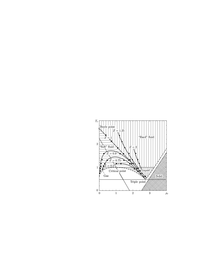
Figure 3: $T$–$\rho$ diagram for gases corresponding to simple liquids; $T_{r}=T/T_{\text{cr}}$ and $\rho_{r}=\rho/\rho_{\text{cr}}$. The line $Z=\frac{PV}{NT}=1.0$ (Zeno line) on the phase diagram. For states with $Z>1.0$ (hard fluids), the repulsive forces dominate. For states with $Z<1.0$ (soft fluids), the attractive forces dominate. The dotted line passing to the critical point and ending at the triple point is the binodal (cf. Fig. 8).

Figure 4: $T$–$\rho$ diagram for water.

The Zeno line is precisely a straight line in the van der Waals model. Using only heuristic considerations for the Lennard–Jones interaction potential, one can show that this curve is almost a straight line indeed. These considerations are of purely physical nature and use the existence of the so-called thermal attractive potential.

Although the considerations presented here are not mathematically rigorous, they elucidate some physical phenomena anew. The Boyle temperature $T_{B}$ and some other quantities usually defined by using the van der Waals model are treated here in a new way. Despite the fat that the logical reasoning is not rigorous, it still perfectly agrees with the above rigorous conception. One can prove in a mathematically rigorous way that the existence of a Zeno line (as a segment of a straight line) can be regarded for pure gases as an additional axiom, which can only be supported by heuristic considerations.

3.1 Heuristic Considerations. The Role of Small Viscosity

Following Clausius, experts in molecular physics usually argue by proceeding from the symmetry of the motion of a molecule averaged in all six directions. In the scattering problem, we use the principle of symmetry in all directions, which is standard in molecular physics, but apply it to define not the mean free path, but other molecular physics quantities. Therefore, the fraction of all particles that moves head-on is 1/12. There are three such directions; hence, one quarter of all molecules collide.

For the interaction potential, we consider the Lennard–Jones potential

$$u(r)=4\varepsilon\Big{(}\frac{a^{12}}{r^{12}}-\frac{a^{6}}{r^{6}}\Big{)},$$ (37)

where $\varepsilon$ is the energy of the depth of the well and $a$ is the effective radius.

In the absence of an external potential, the two-particle problem reduces to the one-dimensional radial-symmetric one.

Recall this passage.

Consider the two-body problem for particles of the same mass. Let us pass to the new variables,

$$r=r_{2}-r_{1},\qquad R=\frac{r_{1}+r_{2}}{2}.$$

This gives

$$r_{1}=R-r,\qquad r_{2}=R+r.$$ (38)

In the new variables, the kinetic energy is

$$T=\frac{m}{2}\dot{R}^{2}+\frac{\mu}{2}\dot{r}^{2},$$ (39)

where $\mu=m/2$ is the reduced mass of the system. Obviously, $\dot{r}=\dot{r}_{2}-\dot{r}_{1}$ is the relative velocity. The first summand in 39 is the kinetic energy of the relative motion of a “$\mu$-point.” The angular momentum of the system is

$$M=m[R\cdot\dot{R}]+\mu[r\cdot\dot{r}].$$ (40)

In the new variables, the Lagrangian becomes

$$L(r,R,\dot{r},\dot{R})=\frac{m}{2}\dot{R}^{2}+\frac{\mu}{2}\dot{r}^{2}-U(r),$$ (41)

where $U(r)$ stands for the interaction potential.

Suppose that, as $t\to-\infty$, the velocities of the structureless particles are equal to ${\mathbb{v}}_{1}^{\mathrm{in}}$ and ${\mathbb{v}}_{2}^{\mathrm{in}}$. This means that, as $t=-\infty$, the trajectories of the particles approach straight lines. In terms of the variable $r=r_{2}-r_{1}$, as $t\to-\infty$, the radius vector of the $\mu$-point asymptotically approaches the function $r^{\mathrm{in}}=\rho+{\mathbb{v}}^{\mathrm{in}}t$, where $\rho{\mathbb{v}}^{\mathrm{in}}=0$ and ${\mathbb{v}}^{\mathrm{in}}={\mathbb{v}}_{2}^{\mathrm{in}}-{\mathbb{v}}_{1}^{\mathrm{in}}$.

The constant vector $\rho$ is the impact parameter. The quantity $\rho$ is equal to the distance between the straight lines along which the particles would move in the absence of the interaction. After the collision, as $t\to\infty$, the velocities of the particles are equal to ${\mathbb{v}}_{1}^{\mathrm{out}}$ and ${\mathbb{v}}_{2}^{\mathrm{out}}$. This means that the radius vector $r(t)$ asymptotically approaches the function ${\mathbb{r}}^{\mathrm{out}}=c+{\mathbb{v}}^{\mathrm{out}}t$. The trajectories ${\mathbb{r}}^{\mathrm{in}}(t)$ and ${\mathbb{r}}^{\mathrm{out}}(t)$ are straight lines. They are referred to as the incoming and outgoing asymptotes, respectively. The value of the relative velocity in the in- and out-states in preserved, namely, $|{\mathbb{v}}^{\mathrm{in}}|=|{\mathbb{v}}^{\mathrm{out}}|=v$.

The scattering process can be represented in the form of the transformation

$${\mathbb{v}}^{\mathrm{in}}\to{\mathbb{v}}^{\mathrm{out}}={\mathbb{n}}v,$$ (42)

where $\mathbb{n}$ stands for the unit vector determining the kinematics of the scattering.

According to the initial conditions,

$$\mathbb{M}=\mu[{\mathbb{r}}\cdot{\mathbb{v}}],\qquad E=\frac{\mu}{2}v^{2}.$$

Since ${\mathbb{M}}r=0$, it follows that the trajectory belongs to the plane of the vectors $\mathbb{r}$ and $\mathbb{v}$. In the polar coordinates $r$, $\chi$, the incoming asymptote corresponds to the value $\chi=0$.

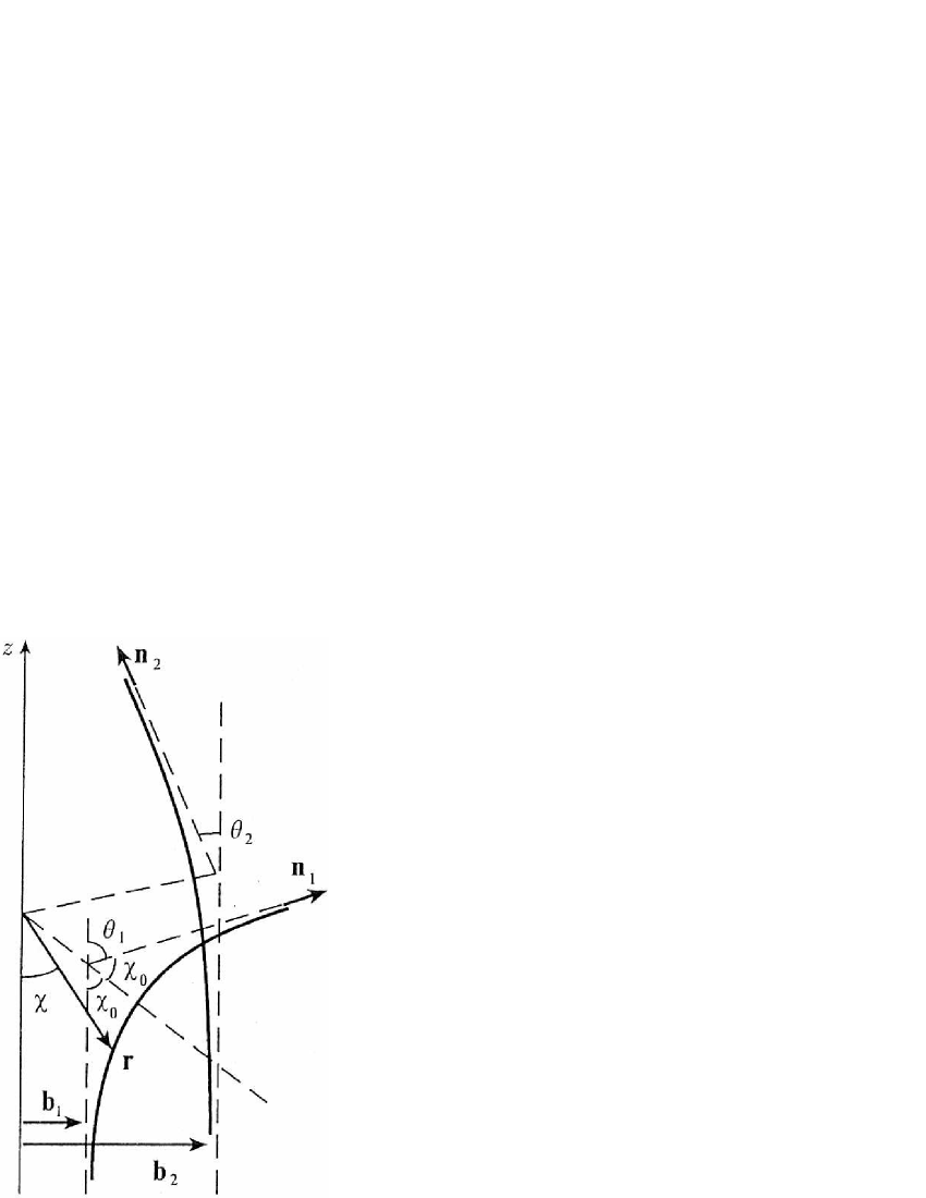
Figure 5: Scattering for the Lennard–Jones potential.

The function $r(\chi)$ decreases, as $\chi$ increases, until it attains the maximal value $r_{\max}=r_{0}$ at $\chi=\chi_{0}$, where the radial component of the velocity vanishes. The outgoing asymptote corresponds to the value $\chi=2\chi_{0}$. Both asymptotes are placed symmetrically with respect to the line passing through the origin and the point of the trajectory which is the nearest to the origin. In dependence on the value of the impact parameter $b$, the possible values of $\chi_{0}$ are in the interval $(0,2\pi)$. The observed angle of scattering $\theta$, which is measures in the interval $(0,\pi)$ by definition, is equal to $\theta=|\pi-2\chi_{0}|$. In Fig. 5, we show the incoming and outgoing asymptotes in the case of Lennard–Jones potential energy. The repulsion corresponds to the value $\rho_{1}$ and the attraction to the value $\rho_{2}$ [56].

Two quantities are preserved in this problem, namely, the energy $E$ and the momentum $M$. In the scattering problem, it is more convenient to consider another constant (which is thus also preserved) instead of the momentum $M$, namely, $b=\sqrt{m}\rho$, where $\rho$ stands for the impact parameter; thus,

$$M=\sqrt{E}b.$$ (43)

Resolving the well-known relation

$$E=\frac{p^{2}}{m}+\frac{M^{2}}{2mr^{2}}+u(r)$$ (44)

with respect to the energy $E$, we obtain the attractive Hamiltonian $H$,

$$H=\frac{p^{2}/(2m)+u(r)}{1-b^{2}/r^{2}},\qquad a<r\leq b.$$ (45)

This simple transformation, if we take the influence of the small viscosity into account, enables us to modify the standard scattering problem in such a way that both the quantity $T_{B}$ and the quantity $T_{\mathrm{c}}$ obtain a new meaning.

The phenomenon which we have described above by using the example of wells is actually a continuous process (which is established for a given temperature) of random creation of dimers and cleaving of dimers by quick monomers. We may speak only of the percent of dimers at a given temperature.

The repulsive Hamiltonian is separated from $H$ by a barrier. Repulsive particles make obstacles in the way of particles of the Hamiltonian $H$, by creating a “viscosity.”

As the temperature decreases, the height of the barrier grows up to the value $E_{\mathrm{cr}}=0.286\varepsilon$, and then starts reducing (see Fig. 6). According to rough energy estimates  [58], for lesser temperatures, an additional barrier must be formed as the clusters are created.

This barrier can be given for neutral gases and methane by germs of droplets, i.e., three-dimensional clusters that contain at least one molecule surrounded by other molecules (a prototype of a droplet).

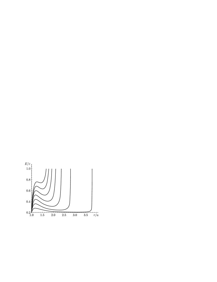
Figure 6: The values of $E(b,r)$ for diverse values of the impact parameter (from left to right): 1.81378, 1.89344, 2.00178, 2.1559, 2.39252, 2.80839, and 3.79391. The critical point is not shown; the minimum disappears at $\rho=1.75441$.

However, to study the penetration through the barrier of the incident particle, we must plot $E$ along the $y$ axis and turn the wells upside down. Then the minimum becomes the barrier and the maximum becomes the depth of the well (see Fig. 7).

Figure 7: The trap for a fictitious particle in the the center of mass coordinate system. The radius vector $r$ of the $\mu$-point is marked on the abscissa axis. The particle falls from the left from the point $r=b$, where $b$ stands for the impact parameter. In the original problem 43 (before the change of variables $M=\sqrt{E}b$), the relation $r=b$ is attained as $r\to\infty$.

A dimer can be formed in a classical domain if the scattering pair has an energy equal to the barrier height, slipping into the dip in “infinite” time and getting stuck in it as the result of viscosity (and hence of some small energy loss), because this pair of particles, having lost energy, hits the barrier on the return path. If the pair of particles has passed above this point, then the viscosity may be insufficient for the pair to become stuck: such a pair returns above the barrier after reflection. Therefore, only the existence of a point $E=E_{\max}$ plus an infinitesimal quantity, where $E_{\max}$ is the upper barrier point, is a necessary condition for the pair to be stuck inside the dip; $E_{\max}^{\mathrm{cr}}$ is the height of the maximum barrier.

We can compare the values $T_{\mathrm{cr}}$ with the values $E_{\max}^{\mathrm{cr}}$ in the table below.

Substance	$\varepsilon$, K	$T_{cr}/4$	$E_{cr}\cdot\varepsilon/k$
$Ne$	36.3	11	10.5
$Ar$	119.3	37	35
$Kr$	171	52	50
$N_{2}$	95,9	31	28
$CH_{4}$	148.2	47	43

Above the value $E_{\text{B}}=0.8\varepsilon$, the trap disappears. At the value $0.286\varepsilon$, the depth of the trap is maximal and corresponds to $T_{\mathrm{cr}}=\frac{1.16\varepsilon}{k}$. For neon and krypton, as can be seen from the table, the concurrence is sufficiently good. Because $T_{B}=3.2\varepsilon/k$, it follows that $T_{B}/T_{\mathrm{cr}}=2.7$, which corresponds to the known relation of “the law of corresponding states” [59].

The temperature corresponding to $4E_{\text{B}}/k$, is the temperature above which dimers do not appear. Exactly this is what we call the Boyle temperature (in contrast to [11]).

In fact, an application of the Clausius approach to pairwise interaction gives a pairwise interaction with respect to the Lennard–Jones potential for two Gibbs ensembles of noninteracting molecules. This leads to the presence of a small friction for a single pair.

The difference $E_{\max}-E_{\min}$ is equal to the energy needed for a particle lying at the bottom of the potential well to overcome the barrier. The value $E_{\max}$ corresponds to the temperature given by $E_{\max}=RT$, where $R$ stands for the universal gas constant. According to graph 6, $E_{\min}$ corresponds to the energy $PV$. Therefore, $E_{\min}/E_{\max}\leq 1$ is the compressibility factor, $Z=PV/RT$. The temperature at the point $E_{\min}=E_{\max}$ is equal to the Boyle temperature.

The dressed or “thermal” potential $\varphi(r)$ is attractive [60]. In addition, because the volume $V$ is a large parameter, it follows that, if the quantity $\varphi(r)=({N\varepsilon a}/{\root 3 \of{V}})U\big{(}r/{\root 3 \of{V}}\big{)},$ where $U\big{(}r/{\root 3 \of{V}}\big{)}$ is a smooth function and $N$ stands for the number of particles, is expanded in terms of $1/\root 3 \of{V}$, then

$$U\Big{(}\frac{r}{\root 3 \of{V}}\Big{)}=C_{1}+\frac{C_{2}r}{\root 3 \of{V}}+\frac{C_{3}r^{2}}{(\root 3 \of{V})^{2}}+O\bigg{(}\frac{1}{(\root 3 \of{V})^{3}}\bigg{)}.$$ (46)

Expanding

$$C_{1}+r^{2}=\frac{(r-r_{0})^{2}}{2}+\frac{(r+r_{0})^{2}}{2},$$ (47)

where $C_{1}=r_{0}^{2}$, we can separate the variables in the two-particle problem as above and obtain the scattering problem for pairs of particles and the problem of their cooperative motion for $r_{1}+r_{2}$. The term $C_{2}r/\root 3 \of{V}$ does not depend on this problem and the correction $({a\varepsilon}/{\root 3 \of{V}})NO\big{(}1/V\big{)}$ is small.

Then, in the scattering problem, an attractive quadratic potential (inverted parabola multiplied by the density or, to be more precise, by the concentration, which we denote by the symbol $\rho$ as well, because the target parameter does not occur below) is added to the Lennard–Jones interaction potential.

For this problem, we can find just as in 44–45, for all $\rho=N/V$, a point corresponding to the temperature at which the well capturing the dimers vanishes, and thus determine the so-called Zeno line. It is actually a straight line (up to 2%), on which $Z=E_{\min}/E_{\max}=1$ (i.e., an ideal curve).

Let us clarify this fact in more detail.

We can treat the repulsing potential as a potential creating a small viscosity.

Let us find the total energy of the attractive Hamiltonian,

$$E=\bigg{(}\frac{mv^{2}}{2(1-b^{2}/r^{2})}\bigg{)}+\frac{\Phi(r)}{1-b^{2}/r^{2}}\,,\qquad\Phi(r)=u(r)-\rho r^{2}.$$

The first term is negative for $r\leq b$ and the other term is positive for $b>r>a$ (i.e., the more is the speed, the less is energy). The mean speed is temperature.

Let us make the change of variables

$$\frac{r}{a}=r^{\prime},\qquad\frac{b}{a}=\widetilde{b},$$

and get rid of $a$. In what follows, we omit both the tilde and the prime.

For a given $b$, the minimum $r_{1}$ and the maximum $r_{2}$ (see the graph no. 1 in [61]) are defined by the relation

$$\frac{dE}{dr}=0.$$ (48)

This gives $E_{\max}$ and $E_{\min}$. These values coincide at some point $b=b_{0}$, and hence

$$\frac{d^{2}E}{dr^{2}}=0$$ (49)

at the point $r_{0}$, i.e., $E_{\max}=E_{\min}$, and this is the very Zeno line.

Let us construct the curve $Z_{\min}=E_{\min}/E_{\max}$ minimal with respect to the target parameter as a function of $\rho$. Let us find the point $Z=E_{\min}/E_{\max}$ for $E_{\max}=E_{\max}^{\mathrm{cr}}$ and find the corresponding point on the curve $Z_{\min}(\rho)$. This point is equal to $Z_{\text{cr}}=0.29$, i.e., to the critical value of the compressibility factor $Z$ for argon.

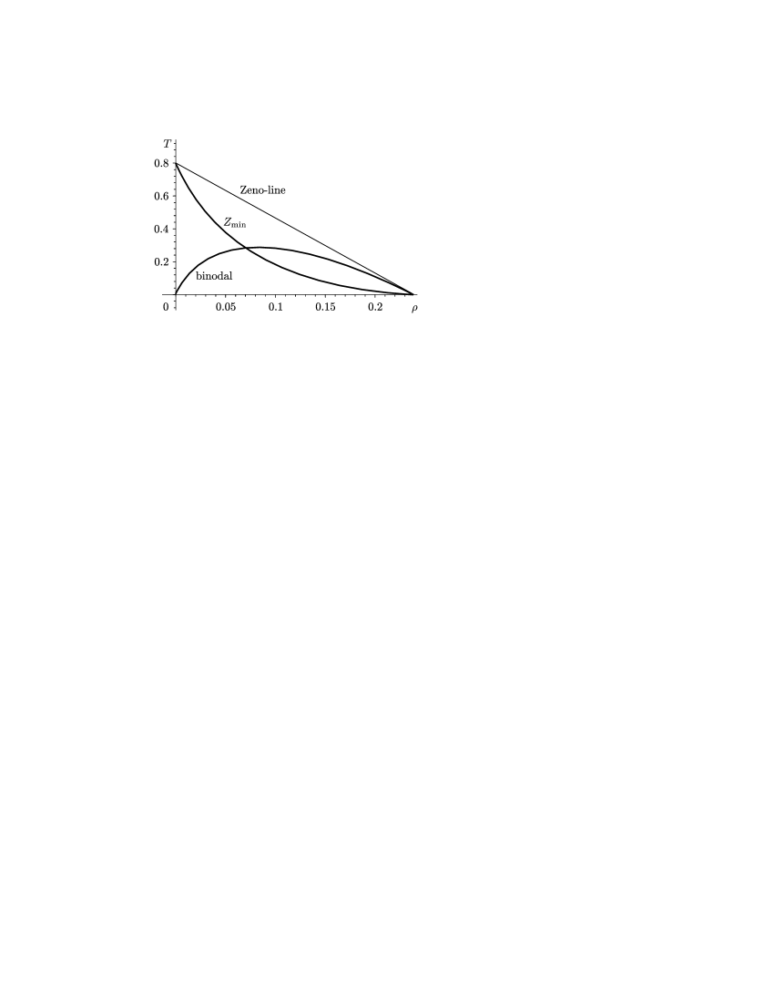
Figure 8: The binodal, the Zeno line, and the curve $Z_{\min}$. This heuristic binodal does not coincide with the experimental one, whereas the Zeno line and $Z_{\mathrm{cr}}$ are close to the corresponding experimental curves.

In order to obtain a binodal according to some “heuristic principle,” we must subtract the curve $Z_{\min}(\rho)$ [62] from the Zeno line. This gives the graph shown in Fig. 8.

3.2 Consideration of Interaction: Nonideal Gas

At first glance, it looks as if the notion of new ideal gas replaces the famous relation, which was approved for many years,

$$PV=NT$$ (50)

(which, moreover, served as an analogy for the main economical law, Irving Fisher’s formula; which is used to calculate the “turnover rate” of capital [63]). This could be surprising indeed. However, this is not the case. The relation $PV=NT$ or, equivalently, $PV=RT$ (because the number of particles in the vessel remains the same) defines an imperfect gas and, in contemporary experimental thermodynamical diagrams, it is called the Zeno line or, sometimes, the “ideal curve,” the “Bachinskii parabola,” or the orthometric curve.

On the diagram $(\rho,T)$ for pure gases, this is the straight line $Z=1$. This line is a most important characteristic feature for a gas which is imperfect. Since, for imperfect gases, it has been calculated experimentally and is an “almost straight” line on the $(\rho,T)$ diagram, it follows that the Zeno line is determined by two points, $T_{B}$ and $\rho_{B}$, called the “Boyle temperature” and the “Boyle density.” In contrast to $Z_{\mathrm{cr}}$, these points are related to the interaction and scattering of a pair of gas particles in accordance with the interaction potential specific for this gas, as was shown in Section 1 and in other papers of the author (see, e.g., [64]). Therefore, the Zeno line on which the relations

$$PV=NT,\qquad\frac{\rho}{\rho_{B}}+\frac{T}{T_{B}}=1,\qquad\frac{N}{V}=\rho,$$ (51)

are satisfied, where $\rho$ is the density (the concentration), is a consequence of pairwise interaction, and thus is a relation for an imperfect gas.

The correction related to the existence of the Zeno line leads to a differential equation [65] whose numerical solution yields an alteration to the gas spinodal for every particular pure gas. For argon and $CO_{2}$, this modification is shown in Fig. 9.

The distribution of number theory, as opposed to the “Bose–Einstein distribution,” does not contain the volume $V$. Let us consider the distribution of number theory multiplied by unknown function $\varphi_{\gamma_{0}}(V)$ which does not vary for $\gamma\geq\gamma_{0}$ and $T\leq T_{\mathrm{cr}}$. Then it follows from 51 that

$$P=\frac{\varphi^{\prime}_{\gamma_{0}}(V)T^{\gamma_{0}+2}}{\Gamma(\gamma_{0}+2)}\int^{\infty}_{0}\frac{\varepsilon^{\gamma_{0}+1}\,d\varepsilon}{e^{-\kappa}e^{\varepsilon}-1},\qquad\varphi^{\prime}_{\gamma_{0}}=\frac{d\varphi_{\gamma_{0}}}{dV},$$ (52)

$$\varphi_{\gamma_{0}}^{\prime}(V)\operatorname{Li}_{\gamma_{0}+2}(y)=\frac{\rho}{T_{B}^{\gamma_{0}+1}\big{(}1-\frac{\rho}{\rho_{B}}\big{)}^{\gamma_{0}+1}},\quad\rho=\frac{R}{V},\quad y=e^{\kappa},\quad\kappa=\frac{\mu}{T}.$$

The differential equation for $\varphi_{\gamma_{0}}$ is

$$\frac{V\varphi^{\prime}_{\gamma_{0}}(V)}{\varphi_{\gamma_{0}}(V)}\frac{\operatorname{Li}_{\gamma_{0}+2}(y)}{\operatorname{Li}_{\gamma_{0}+1}(y)}=1,\qquad V=\frac{R}{\rho}.$$ (53)

See Fig. 9.

Figure 9: The dotted line shows the Zeno line $Z=1$. The bold line is the critical isotherm of an imperfect gas (argon) calculated theoretically; the thin lines correspond to the isochores of an imperfect gas for $T<T_{\mathrm{cr}}$. Their initial points lie on the gas spinodal.

Remark 5.

The notion of Lagrangian manifold, which is the “equation of state” defining a two-dimensional surface in the four-dimensional phase space, which was introduced by the author in [69] (see MSC2010 (Mathematics Subject Classification 2010) http://www.ams.org/msc/, the section “53D12 Lagrangian submanifolds; Maslov index”) enables one to carry out this multiplication by the function $\varphi_{\gamma_{0}}(V/{V_{0}})$ without violating the Lagrangian property, and thus the basic relationships for the free energy, internal energy, and thermodynamical potential are preserved.

4 Ideal liquid

Let us now pass to the notion of ideal liquid. For an expert in mathematical physics, an ideal liquid is an incompressible liquid. In our mathematical conception of thermodynamics, we shall abide by this definition. In this case, on the Zeno-line on the plane $\{P,Z\}$, for $Z=1$, the point $P(T,\rho)$ in 51 is defined uniquely. The isotherm $T=\text{const}$ is a straight line. The second point is obviously the spinodal point.

As is well known, the passage from the gaseous state to the liquid one is accompanied by an entropy drop. Naturally, the entropy, which determines the measure of chaotic behavior, is less for the liquid state than for the gaseous state. At the same time, the general property of “choosing” a subsystem with the greatest chaoticity among all possible subsystems leads to the property of constant entropy of the liquid, which was noted both theoretically and experimentally, even if the temperature tends to the absolute zero ([67, 68]) (the entropy tends to $\log 2$).

In our model of ideal liquid as an incompressible liquid, we suppose in addition that the maximum of the entropy on a given isotherm (i.e., as $\mu\to 0$) does not vary when the temperature varies.

The big thermal potential is of the form

$$\Omega=-PV_{\gamma}=-\frac{\pi^{\gamma+1}V_{\gamma}T}{\Lambda^{2(1+\gamma)}}\frac{1}{\Gamma(2+\gamma)}\int_{0}^{\infty}\frac{t^{1+\gamma}\,dt}{(e^{t}/z)-1}=\frac{-\pi^{\gamma+1}V_{\gamma}T^{2+\gamma}}{\Lambda^{2(1+\gamma)}}\operatorname{Li}_{2+\gamma}(z),\quad z=e^{\mu/T},$$ (54)

where $\Lambda$ is a constant, its own for every substance (as a rule, it depends on mass; however, we try to avoid mass by passing from density to concentration).

According to [11] the entropy is of the form

$$S=-\bigg{(}\frac{\partial\Omega}{\partial T}\bigg{)}_{V,\mu}=(2+\gamma)\frac{T^{1+\gamma}}{\Lambda^{2(1+\gamma)}}\operatorname{Li}_{2+\gamma}(z)-\frac{T^{1+\gamma}}{\Lambda^{2(1+\gamma)}}\operatorname{Li}_{1+\gamma}(z)\frac{\mu}{T}$$

$$=\frac{\pi^{\gamma+1}T^{1+\gamma}}{\Lambda^{2(1+\gamma)}}\Big{[}(2+\gamma)\operatorname{Li}_{2+\gamma}(z)-\operatorname{Li}_{1+\gamma}(z)\frac{\mu}{T}\Big{]}.$$ (55)

The maximum at $\mu=0$ is

$$S_{\mu=0}=\Big{(}\frac{\pi}{\Lambda^{2}}\Big{)}^{\gamma+1}(2+\gamma)\zeta(\gamma+2)T^{\gamma+1}.$$ (56)

We are interested in in the case $\gamma<0$ as well.

Thus, we have two unknown constants, namely, $\Lambda$ and the value of the entropy $S_{\mu=0}=\operatorname{const}$ . These two constants can be defined from the experimental value of the critical point of the liquid phase at the negative pressure (see Section 6 below), namely, from the minimum point of the pressure for a given simple liquid of the value $\gamma$ at this point and from the temperature. This point is absent in the van der Waals model. This point is present in our model of liquid phase.

For example, for water, we obtain $S_{\mu=0}=3.495$ and $\Lambda=3.74$. However, the computation is carried out under the assumption that the Zeno-line is a line segment, whereas this segment becomes curvilinear for water at low temperatures (see Fig. 4).

According to the van der Waals conception, we normalize as follows:

$$T^{\mathrm{red}}=\frac{T}{T_{\mathrm{cr}}},\qquad P^{\mathrm{red}}=\frac{P}{P_{\mathrm{cr}}}.$$ (57)

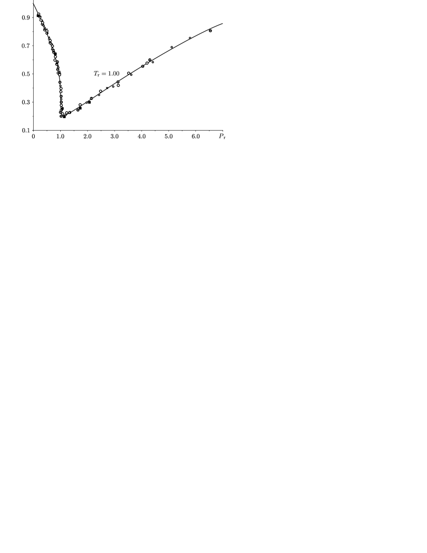
Figure 10: Experimental graph for the different gases, including those for methane, ethylene, ethane, propane, $n$-butane, isopentane, $n$-heptane, nitrogen, carbon dioxide, and water. Each gas is equipped with a particular symbol on the graph.

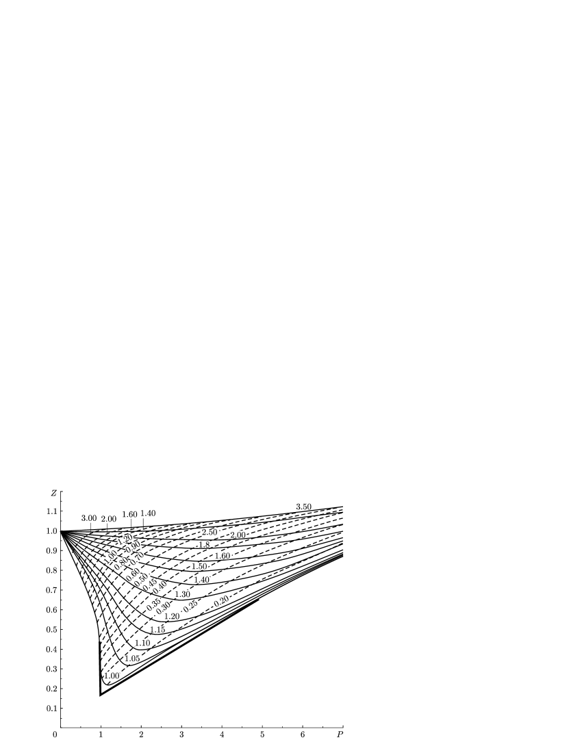
Figure 11: The continuous lines are the experimental isotherms for $T\geq T_{\mathrm{cr}}$ for methane, and the dotted lines are experimental isochors. The theoretical critical isotherm coincides with the experimental isotherm up to $Z=0.29$ and is continued by a straight line up to the point $P=1$, $Z=1/\rho_{0}=0.14$ (see 58, 59). Further, at an acute angle, a tangent to the experimental isotherm at a point of Zeno-line is drawn. The straight line from the point $P=1,Z=0.14$ to the point of tangency is the critical isotherm of the ideal liquid phase. It can be seen by comparing the figure with Fig. 10, the theoretical isotherm thus obtained corresponds to the isotherm of the “law of corresponding states” for the gases indicated in Fig. 10.

Denote by $\rho_{0}$ the solution of the equation

$$\frac{1}{T_{B}^{\mathrm{red}}}+\frac{\rho}{\rho_{B}}=1,$$ (58)

where $T_{B}$ stands for the Boyle temperature and $T_{B}^{\text{red}}=\frac{T_{B}}{T_{\text{cr}}}$ is a dimensionless quantity, $T^{\text{red}}=\frac{T}{T_{\text{cr}}}$. Then

$$\frac{\rho_{0}}{\rho_{B}}=1-\frac{1}{T_{B}^{\mathrm{red}}},\qquad\rho_{B}^{\mathrm{red}}=\frac{\rho_{B}}{\rho_{0}}.$$ (59)

Hence, the locus of the spinodal points  is given by the formula

$$P^{\mathrm{red}}=\frac{1}{\Big{(}1-\frac{1}{T_{B}^{\mathrm{red}}}\Big{)}}T^{\mathrm{red}}\Big{(}1-\frac{T^{\mathrm{red}}}{T_{B}^{\mathrm{red}}}\Big{)}Z(\gamma).$$ (60)

Hence, for $\gamma>0$,

$$Z_{\mathrm{cr}}^{\gamma(T^{\mathrm{red}})}=\frac{\zeta(2+\gamma(T^{\mathrm{red}}))}{\zeta(1+\gamma(T^{\mathrm{red}}))}.$$ (61)

Recall that $\gamma(T)$ can be calculated from the algebraic relation $S_{\mu=0}=\mathrm{const}$.

If we use the Maxwell condition which states that the transition from gas to liquid occurs for the same chemical potential, pressure, and temperature, then we can construct the so-called binodal. The binodal thus constructed coincides with the experimental one, in contrast to the van der Waals binodal (Fig. 1 (b)) and to the binodal presented in Fig. 8.

5 Negative pressure and a new critical point of possible transition from liquid to “foam”

First of all, using the Wiener quantization of thermodynamics, we shall now clarify why in Section 4 we have derived the condition $S|_{\mu=0}=\text{const}$, where the constant does not depend on the temperature, from the model of incompressible fluid.

By the Bachinskii relation on the Zeno line, the model of incompressible fluid leads to a rigid relationship between the density (the concentration) $\rho$ and the temperature. Since the value $N$ is undefined for $\mu=0$ (i.e., the concentration $\rho$ is undefined), it follows that the temperature is undefined as well and, by the indeterminacy principle, the entropy takes a constant value and can be defined. (Note in addition that, for $\mu=0$, the activity is equal to one for any (undefined) temperature.) This very fact means that $S|_{\mu=0}=\text{const}$. As we shall see below, the value of this constant is uniquely defined by the new critical point of transition from the liquid to a “foam” (a disperse state, [58]). The value of the same point also defines the constant $\Lambda$ in the definition of $\Omega$, and thus, after computing $\varphi_{\gamma}(V/V_{\text{cr}})$, one can completely describe the distribution function for the gaseous branch in thermodynamics. Note that the indeterminacy at the spinodal point agrees with the experiments of the Academician Skripov and his school on the absolute instability of the spinodal point.

Let us now proceed with negative values of $Z$.

As is known, the Bose–Einstein distribution is obtained as the sum of terms of an infinitely decreasing geometric progression. If the progression is bounded by the number $N$, then the potential becomes

$$\Omega=-T\sum_{k}\log\bigg{(}\frac{1-\exp\frac{\mu-\varepsilon_{k}}{T}N}{1-\exp\frac{\mu-\varepsilon_{k}}{T}}\bigg{)}.$$ (62)

What is the relationship  between $E_{i}$ and $\gamma$?

(1) Ultrarelativistic case. Here $E=cp$.

$$E_{i+1}-E_{i}=\int_{E_{i}}^{E_{i+1}}cp\,p^{2}\,dp=\frac{1}{4}\bigg{(}p^{4}(E_{i+1})-p^{4}(E_{i})\bigg{)}\sim\frac{3}{4}cp^{3}(E_{i}^{i+1})=\frac{3}{c^{2}}(E_{i}^{i+1})^{3}.$$ (63)

(2) Nonrelativistic case. Here $E=\frac{p^{2}}{2m}$.

$$E_{i+1}-E_{i}=\int_{E_{i}}^{E_{i+1}}\frac{p^{2}}{2m}p^{2}\,dp=\frac{1}{2m}\bigg{(}\frac{p^{5}}{5}(E_{i+1})-\frac{p^{5}}{5}(E_{i})\bigg{)}$$ (64)

$$\frac{1}{2m}\bigg{(}\frac{(\sqrt{2mE_{i+1}})^{5}}{5}-\frac{(\sqrt{2mE_{i}})^{5}}{5}\bigg{)}\cong\mathrm{const}(E_{i}^{i+1})^{3/2}.$$

(3) Consideration of the degrees of freedom. $E=\frac{p^{2+\sigma}}{2mp_{0}}$. Here

$$E_{i+1}-E_{i}=\int_{E_{i}}^{E_{i+1}}\frac{p^{2+\sigma}}{2m}p^{2}\,dp\cong\mathrm{const}(E_{i}^{i+1})^{(4+\sigma)/(2+\sigma)}.$$ (65)

By 13,

$$\gamma=\frac{1-\sigma}{2+\sigma}$$

and thus $\gamma<0$ for $\sigma>1$.

As was proved in [13--14], passing to the limit in the Euler–Maclaurin formula, we have proved that

$$N=\frac{1}{(\gamma+1)\Gamma(\gamma+1)}\int_{0}^{\infty}\left\{\frac{1}{e^{b\xi}-1}-\frac{N}{e^{Nb\xi}-1}\right\}\,d\xi^{\alpha}.$$ (66)

In particular, for $\gamma=-1/2$,

$$N=\frac{1}{\Gamma(3/2)}\int_{0}^{\infty}\left\{\frac{1}{e^{b\xi^{2}}-1}-\frac{N}{e^{Nb\xi^{2}}-1}\right\}\,d\xi.$$ (67)

The absolute value of the derivative of the integrand can readily be estimated by using the identities presented below. By the Euler–Maclaurin bounds, this shows that one can pass from the sums of the form 62 to the corresponding integrals with the accuracy needed here.

Hence, writing $N_{\operatorname{cr}}=k_{0}$, we obtain the following formula for the integral at $\mu=0$:

$$\mathcal{E}=\frac{1}{\alpha\Gamma(\gamma+2)}\int\frac{\xi\,d\xi^{\alpha}}{e^{b\xi}-1}=\frac{1}{b^{1+\alpha}}\int_{0}^{\infty}\frac{\eta d\eta^{\alpha}}{e^{\eta}-1},$$ (68)

where $\alpha=\gamma+1$. Therefore,

$$b=\frac{1}{\mathcal{E}^{1/(1+\alpha)}}\left(\frac{1}{\alpha\Gamma(\gamma+2)}\int_{0}^{\infty}\frac{\xi\,d\xi^{\alpha}}{e^{\xi}-1}\right)^{1/(1+\alpha)}.$$ (69)

We obtain

$$\int_{0}^{\infty}\left\{\frac{1}{e^{b\xi}-1}-\frac{k_{0}}{e^{k_{0}b\xi}-1}\right\}\,d\xi^{\alpha}=\frac{1}{b^{\alpha}}\int_{0}^{\infty}\left(\frac{1}{e^{\xi}-1}-\frac{1}{\xi}\right)\,d\xi^{\alpha}$$ (70)

$$\quad+\frac{1}{b^{\alpha}}\int_{0}^{\infty}\left(\frac{1}{\xi}-\frac{1}{\xi(1+(k_{0}/2)\xi)}\right)\,d\xi^{\alpha}-\frac{k_{0}^{1-\alpha}}{b^{\alpha}}\int_{0}^{\infty}\left\{\frac{k_{0}^{\alpha}}{e^{k_{0}\xi}-1}-\frac{k_{0}^{\alpha}}{k_{0}\xi(1+(k_{0}/2)\xi)}\right\}\,d\xi^{\alpha}.$$

Write

$$c=\int_{0}^{\infty}\left(\frac{1}{\xi}-\frac{1}{e^{\xi}-1}\right)\xi^{\gamma}\,d\xi.$$

After the change $k_{0}\xi=\eta$, we see that

$$\frac{k_{0}^{1-\alpha}}{b^{\alpha}}\int_{0}^{\infty}\left\{\frac{k_{0}^{\alpha}}{e^{\eta}-1}-\frac{k_{0}^{\alpha}}{\eta(1+\eta/2)}\right\}\,d\xi^{\alpha}=\frac{k_{0}^{1-\alpha}}{b^{\alpha}}\int_{0}^{\infty}\left\{\frac{1}{e^{\eta}-1}-\frac{1}{\eta(1+\eta/2)}\right\}d\eta^{\alpha}$$

$$\qquad=\frac{k_{0}^{1-\alpha}}{b^{\alpha}}\left\{\int_{0}^{\infty}\left(\frac{1}{e^{\eta}-1}-\frac{1}{\eta}\right)+\int_{0}^{\infty}\frac{d\eta^{\alpha}}{2(1+\frac{\eta}{2})}\right\}=-c\frac{k_{0}^{1-\alpha}}{b^{\alpha}}+c_{1}\frac{k_{0}^{1-\alpha}}{b^{\alpha}}\,.$$ (71)

Since

$$\frac{1}{\eta(1+\eta/2)}=\frac{1}{\eta}-\frac{1}{2(1+\eta/2)}$$ ,

we can set

$$c_{1}=\int_{0}^{\infty}\frac{d\eta^{\alpha}}{2(1+\frac{\eta}{2})}\,,$$

and write

$$\int_{0}^{\infty}\left(\frac{1}{\xi}-\frac{1}{\xi(1+\frac{k_{0}}{2}\xi)}\right)\,d\xi^{\alpha}=\frac{k_{0}}{2}\int_{0}^{\infty}\frac{\,d\xi^{\alpha}}{1+\frac{k_{0}}{2}\xi}=\left(\frac{k_{0}}{2}\right)^{1-\alpha}\int_{0}^{\infty}\frac{d\eta^{\alpha}}{1+\eta}=c_{1}\left(\frac{k_{0}}{2}\right)^{1-\alpha}.$$ (72)

Hence,

$$-\frac{1}{b^{\alpha}}c_{1}+\frac{1}{b^{\alpha}}c\left(\frac{k_{0}}{2}\right)^{1-\alpha}\!\!\!\!-\frac{k_{0}^{1-\alpha}}{b^{\alpha}}\int_{0}^{\infty}\!\left\{\frac{1}{e^{\eta}-1}-\frac{1}{\eta(1-\frac{\eta}{2})}\right\}d\eta^{\alpha}-\frac{1}{2}\int\!\frac{d\eta^{\alpha}}{1+\frac{\eta}{2}}\cdot\frac{k_{0}^{1-\alpha}}{b^{\alpha}}=-\frac{1}{b^{\alpha}}c+\frac{k_{0}^{1-\alpha}}{b^{\alpha}}c.$$ (73)

Since $k_{0}$ is the number of particles, $b=1/T$, and $\alpha=1+\gamma$, it follows that $k_{0}b^{\alpha}$ for $\gamma>0$ is the value of the Riemann zeta function, $\zeta(1+\gamma)$. Therefore, $k_{0}^{\gamma+1}$ increases for $\gamma<1$, and the first term of the right-hand side of equation 5 can be neglected. Introducing the function

$$\mathcal{M}(\gamma+1)=\bigg{(}\frac{c(\gamma)}{\Gamma(\gamma+1)}\bigg{)}^{\frac{1}{1+\gamma}},$$ (74)

we see that the compressibility factor

$$Z_{\gamma}=-\zeta(\gamma+2)/\mathcal{M}(\gamma+1)$$

is subjected to a flexion   from $\gamma>0$ to $\gamma<0$.

In this case, we obtain another critical point, which fully corresponds to the physical meaning (see [71]).

Thus, if the compressibility factor is negative, then we divide $\mathcal{E}/N$ by $T^{\gamma+1}$ with $\gamma<0$ rather than by $T$, because

$$\frac{\mathcal{E}}{N}\Big{|}_{\mu=0}=\frac{\zeta(\gamma+2)T^{\gamma+2}_{\mathrm{red}}}{\mathcal{M}(\gamma+1)T_{\mathrm{red}}}=T^{\gamma+1}_{\mathrm{red}}\frac{\zeta(\gamma+2)}{\mathcal{M}(\gamma+1)},$$

i.e., the energy evaluated for a single particle at $\mu=0$ (at the “degeneration” point), for $P<0$, is proportional to $T^{\gamma+1}_{\mathrm{red}}$, i.e., to the temperature taken to a power with an exponent less than one. For $P<0$, the compressibility factor becomes a dimensional quantity; however, this is always considered in this very way on curves in the $\{Z,P\}$ space when using the van der Waals normalization 57. Let us now present a graph for negative pressure for the Lennard–Jones potential, where the new critical point is obtained by using a computer experiment.

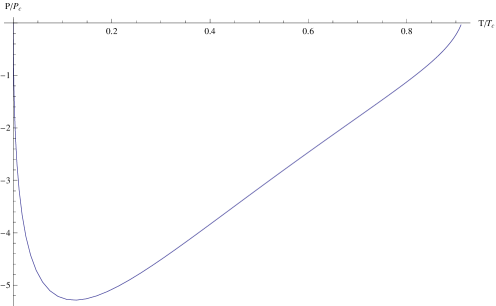
Figure 12: The spinodal in the coordinates given by the temperature $T_{\mathrm{red}}$ and the negative pressure $P_{\mathrm{red}}$.

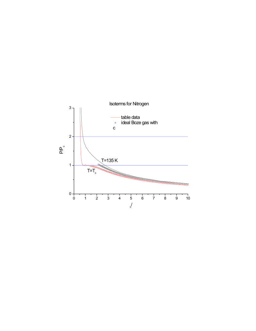
Figure 13: Isotherms for nitrogen, $P/P_{c}$ versus $\rho_{c}/\rho$, ideal Bose gas with $\gamma=0.218$, $Zc=0.287$.

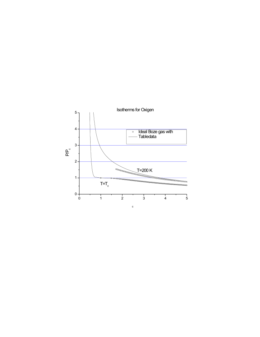
Figure 14: Isotherms for oxygen, $P/P_{c}$ versus $\rho_{c}/\rho$, ideal Bose gas with $\gamma=0.219$.

6 On Homogeneous Mixtures of Gases

When considering a gas mixture, we would like to attract attention at the following fundamental point. As is well known, in statistical physics and thermodynamics, the energy is sometimes connected with the number of degrees of freedom and the temperature; for example, this is the case in the equidistribution law. It turns out in this case that the energy depends on the temperature and on the number of degrees of freedom and does not depend on the mass. The sequential usage of this conception gave us a continuous parameter $\gamma$ related to the fractal dimension in the momentum space. Continuing the use of this conception in the case of a mixture of pure gases, we are to speak of the concentration rather than on the density, i.e., we are to neglect the masses of miscible pure gases.

The sequential application of number theory in thermodynamics, i.e., the consideration of the main axiom for the gas mixture (which was in fact made by experimenters, at least in the case of air (see [71])), leads to the formulas presented below.

If the values of energies $\mathcal{E}_{1}$ and $\mathcal{E}_{2}$ expanded into sums of $N_{1}$ and $N_{2}$ summands, respectively, correspond to fractional dimensions $\gamma_{1}$ and $\gamma_{2}$, respectively, and the values of the pairs $\{\mathcal{E}_{1},N_{1}\}$ and $\{\mathcal{E}_{2},N_{2}\}$ are at the “verge of degeneration,” i.e., adding an excessive number to $N_{1}$ and to $N_{2}$ leads to the “appearance of the Bose condensate,” then, for the sum $\mathcal{E}_{1}+\mathcal{E}_{2}$ and for $N_{1}+N_{2}$, any adding an excessive number to $N_{1}+N_{2}$ also leads to the “appearance of the Bose condensate.”

Let $\rho_{1}^{\mathrm{cr}}$ and $\rho_{2}^{\mathrm{cr}}$ be the critical concentrations (in the units $\mathrm{cm}^{-3}$), and let $N_{1}$ and $N_{2}$ be proportional to the molar concentrations,

$$\frac{N_{1}}{N_{1}+N_{2}}=\alpha,$$ (75)

$$\frac{N_{2}}{N_{1}+N_{2}}=\beta,$$ (76)

$$N=N_{1}+N_{2},\qquad\alpha+\beta=1.$$ (77)

Since

$$\mathcal{E}_{\mathrm{cr}}=\mathcal{E}|_{\mu=0}=N|_{\mu=0}Z^{\mathrm{cr}}\frac{\Gamma(\gamma+1)}{\Gamma(\gamma+2)}T^{\mathrm{cr}}=N^{\mathrm{cr}}Z^{\mathrm{cr}}(\gamma^{\mathrm{cr}}+1)$$

for $\gamma>0$, we see that, dividing the equation

$$\mathcal{E}^{\mathrm{sum}}_{\mu=0}=\mathcal{E}^{(1)}_{\mu=0}+\mathcal{E}^{(2)}_{\mu=0}=N_{1}^{\mathrm{cr}}(\gamma_{1}+1)Z_{1}^{\mathrm{cr}}T_{1}^{\mathrm{cr}}+N_{2}^{\mathrm{cr}}(\gamma_{2}+1)Z_{2}^{\mathrm{cr}}T_{2}^{\mathrm{cr}}$$

by $N_{\text{sum}}^{\text{cr}}$, we obtain the relation

$$(\gamma_{\mathrm{sum}}^{\mathrm{cr}}+1)Z_{\mathrm{sum}}^{\mathrm{cr}}T_{\mathrm{sum}}^{\mathrm{cr}}=\alpha(\gamma^{\mathrm{cr}}_{1}+1)Z^{\mathrm{cr}}_{1}T^{\mathrm{cr}}_{1}+\beta(\gamma^{\mathrm{cr}}_{2}+1)Z^{\mathrm{cr}}_{2}T^{\mathrm{cr}}_{2},$$ (78)

where $Z^{\text{cr}}=\zeta(\gamma+2)/\zeta(\gamma+1)$, the subscripts 1 and 2 denote the first and the second gas of the mixture, respectively, and the subscript sum denotes the gas mixture. Similarly,

$$S=N(Z-\mu/T),$$

since the entropy is additive, when dividing by $N^{\text{sum}}_{\mu=0}$, we obtain the relation

$$Z_{\mathrm{sum}}^{\mathrm{cr}}(\gamma_{\mathrm{sum}}^{\mathrm{cr}}+2)=\alpha(\gamma^{\mathrm{cr}}_{1}+2)Z^{\mathrm{cr}}_{1}+\beta(\gamma^{\mathrm{cr}}_{2}+2)Z^{\mathrm{cr}}_{2}.$$ (79)

It follows from the above two relations that the quantity $\gamma=\gamma_{\mathrm{sum}}$ almost linearly depends also on the values $\alpha$ and $T_{\mathrm{cr}}=T_{\mathrm{cr}}^{\mathrm{sum}}$. This fact is well known as “Kay’s rule” in the phenomenological theory of mixtures. For air, we have $T_{\mathrm{cr}}^{\mathrm{sum}}=232\,\text{K}$, whereas $T_{\mathrm{cr}}=255\,\text{K}$ for oxygen (20% in air) and $T_{\mathrm{cr}}=226\,\text{K}$ for nitrogen (80% in air). The value of $T_{\mathrm{cr}}^{\mathrm{sum}}$ coincides with the value of this quantity evaluated according to the above formulas up to the accuracy of $0.5\%$.

We have defined $Z_{\mathrm{cr}}$ for the ideal gases, and hence also $\gamma_{\mathrm{cr}}$ for a gas mixture. For a mixture of real gases, we must define the function $\varphi_{\gamma}^{\mathrm{mix}}$.

It turns out that, for a mixture, the Zeno-line is not a segment of a straight line, which is the case and is observed experimentally for pure gases. Therefore, for a mixture, it is insufficient to find the values $T_{B}^{\mathrm{mix}}$ and $\rho_{B}^{\mathrm{mix}}$. One must also define the function $\varphi_{\gamma^{\mathrm{cr}}}^{\mathrm{mix}}$. This can be carried out by using the following formulas.

We are interested only in the values of $\mu_{1}$ and $\mu_{2}$ that correspond to the Zeno line of each of the gases (see 52-53).

Since, by assumption, the critical point enters the homogeneity domain, it follows that the concentrations $\alpha$ and $\beta$ are preserved, and hence, using equations 75–77, we obtain the following equation for the sum of the entropies, where $\kappa=\mu/T$:

$$(\gamma_{\mathrm{sum}}+2)Z_{\gamma_{\mathrm{sum}}+2}(e^{\kappa_{\mathrm{sum}}})-\kappa_{\mathrm{sum}}=\alpha\big{\{}(\gamma_{1}+2)Z_{\gamma_{1}+2}(e^{\kappa_{1}})-\kappa_{1}\big{\}}+\beta\big{\{}(\gamma_{2}+2)Z_{\gamma_{2}+2}(e^{\kappa_{2}})-\kappa_{2}\big{\}},$$ (80)

where $Z_{\gamma+2}$ is equal to the ratio $\operatorname{Li}_{\gamma+2}(e^{\kappa})/\operatorname{Li}_{\gamma+1}(e^{\kappa})$.

Recall that the values of $\kappa_{1}$ and $\kappa_{2}$ are taken according to the Zeno lines of the first and the second gas, respectively. Hence, using the given values of $\gamma$, $\gamma_{1}$, and $\gamma_{2}$ obtained from 79, we find the value $\kappa=\kappa_{\mathrm{sum}}$, which defines the function $\varphi_{\gamma}(V)$ by relation 53. This enables us to define the dependence of $T_{\mathrm{cr}}^{\mathrm{sum}}$ for a mixture of real gases.

Remark 6.

We have proved that the Boltzmann distribution, which is based on the fact that transpositions of two particles in a set of $N$ particles lead to a new microscopic state, is based in turn on the dogma of the natural series, and hence cannot be applied to the concept of “pile” as a macroscopic state. This implies that the Maxwell distribution describes the ideal gas too roughly.

The introduction of new parameter $\gamma$ enables one to assign the mean energy of the system with respect to the spectral density of a given molecule with higher accuracy as compared with the similar assignment using the equidistribution law with respect to the degrees of freedom, where only the number of atoms of the given molecule is taken into account. As $\gamma\to\infty$ or $\mu\to-\infty$ (the chemical potential), we obtain the old conception of ideal gas.

Certainly, the interaction of molecules depends on the spectrum of molecules. However, the experiment shows that, for all molecules except for those of water, there are two important constants, $T_{B}$ and $\rho_{B}$, and it turns out that these two constants and the critical value of the compressibility factor are sufficient to describe, with the corresponding accuracy, both the equation of state of a pure gas and that of a gas mixture.

Bohr’s Complementarity Principle, as applied to thermodynamical quantities, enables one to elucidate the notion of critical exponents anew.

7 New approach to independent events in probability theory

As was said above, we consider probability theory without preliminarily passing to the limit

$$p_{i}=\lim_{N\to\infty}\frac{N_{i}}{N};$$

we first consider the system for a finite $N$,

$$M=\sum_{i=0}^{\infty}N_{i}\lambda_{i},\qquad\sum_{i=0}^{\infty}N_{i}=N.$$ (81)

In this system of equations, we pass to the asymptotic behavior as $N\to\infty$ and $M\to\infty$ in such a way that $N$ and $M$ turn out to be connected by a relation corresponding to relation 14 of the present paper. We consider the set of solutions of system 81 as the family of elementary equiprobable events. To be more precise, we consider the solutions of the system of inequalities

$$\sum_{i=0}^{\infty}N_{i}\lambda_{i}\leq M,\qquad\sum_{i=0}^{\infty}N_{i}=N$$ (82)

rather than the system of equations. As is clear from system 13, there is an $N_{c}$ such that the number of solutions of this system is the largest possible, and this number can asymptotically be calculated. The number $M_{c}$ corresponds to $N_{c}$.

One can introduce two Lagrange conjugate quantities, namely, the chemical potential $\mu$ and the inverse temperature $\beta$. The value $\mu=0$ corresponds to the critical values $N_{c}$ and $M_{c}$. Thus, we can transfer all our considerations concerning ideal gases to the new probability theory. Poincaré writes about an insufficiently clear (“obscure”) “instinct which we call common sense” on which probability theory (and, I shall add, the notion of independent events) must be based.

If one starts from the notion of ideal gas as a gas of particles without interaction, then it is natural to assume that independent events are events without interaction. However, when we consider a mixture of ideal gases, then we start from the very absence of interaction between the particles. Since relations 78, 79 express this condition, we must use these very relations.

In this definition of independent events, there is an a priori given probability

$$\alpha=\frac{N_{1}}{N_{1}+N_{2}},\qquad\beta=1-\alpha.$$ (83)

The parameter $\gamma$ is related to the notion of fractal dimension, and thus to the Hausdorff–Besicovitch dimension, and, in this relation, this notion, which has recently been widely used, must necessarily be related to the new probability theory. By the definition in 83, the formulas are of “conditional” nature in the sense appropriate in the ordinary probability theory.

The notion of independence has already been considered in Kolmogorov’s complexity theory and completely agrees with formula 79. As far as formula 80 is concerned, it distinguishes a sufficiently important class in the case of dependent events.

To generalize the new definition of independence of events in the new probability theory, it is necessary to pass first of all from equiprobable elementary events presented above to equipping these events by weights, which is brilliantly done in Vershik’s paper [12], and to a generalization of the new notion of independent events to Vershik’s multiplicative measures. In this case, measure theory, which is the most important element of Kolmogorov’s probability theory, will find an application also to the above new conception of independent events.

8 Application to economics. The theory of crisis of debts

As already stated on numerous occasions, money obeys the “Bose statistics” and banknotes of one denomination, are practically indistinguishable despite their different numbers [3, 81]. Therefore, we can associate the “number” (amount) of money with the number of particles in physics (which is consistent with Irving Fisher’s Correspondence Principle) [72]. In economics, the goods are also averaged. The term “wholesale” is usually used for them, and the term “at retail” can be used only occasionally, for example, for authorized artwork. Fisher’s Correspondence Principle consists in the following comparison of economic and physical quantities:

the volume of goods $Q$ corresponds to the volume of gas $V$;

the price of the amount of goods $P$ corresponds to the pressure $P$;

the amount of money $M$ corresponds to the number of particles $N$;

the turnover rate $V$ corresponds to the temperature $T$.

By Friedman’s rule, the optimal amount of money corresponds to the zero nominal percentage [73]. Combining this with the appropriately modified method of Lagrange indeterminate multipliers, we can regard the nominal percentage $R$ as an addition to the amount of money $M$.

In the same way, the value of the turnover rate $V$ is associated with the degree of uncertainty, or entropy 55, which is an additional quantity:

$$S=\frac{\pi^{\gamma+1}V^{\gamma+1}}{\Lambda^{2(^{\gamma}+1)}}\bigg{\{}(2+\gamma)\operatorname{Li}_{2+\gamma}(z)-\operatorname{Li}_{1+\gamma}(z)\frac{R}{V}\bigg{\}},$$ (84)

where $\Lambda$ is a certain constant, its own for each currency, and $z=e^{R/V}$.

The price of the volume $Q_{\gamma}$ has the form

$$P=\frac{\pi^{\gamma+1}}{\Lambda^{2(^{\gamma}+1)}}V^{\gamma+2}\operatorname{Li}_{2+\gamma}(z).$$ (85)

Now Irving Fisher’s Correspondence Principle can be extended to all the thermodynamic quantities. The ratio

$$\frac{PQ}{MV}\bigg{|}_{R=0}=\frac{\zeta(\gamma+2)}{\zeta(\gamma+1)}$$ (86)

allows us to obtain, for economics, the family of distributions depending on the parameter $\gamma$ once the value of the quantity $({PQ})/{MV}$ is calculated as $R\to 0$.

Irving Fisher had in mind the correspondence which is known today under the title of the “fundamental law of economics,”

$$PQ=MV.$$

In view of 84, this correspondence takes the form

$$PQ=Z_{\mathrm{c}}MV,$$ (87)

where the compressibility factor

$$Z_{\mathrm{c}}=\frac{PQ}{MV}\bigg{|}_{R=0}$$

has its own particular value for each country or region. The introduction of a common currency for a group of countries (or regions) corresponds to the mixing of pure gases (see [36]).

An example of the case of the zero nominal percentage $R$ in the USSR was the post-war reconstruction of industry accompanied by the simultaneous reduction in prices. We see that this corresponds to the maximal entropy as a measure of uncertainty (under a planified socialist economy!). Hence, as the turnover rate $V$ (similar to temperature in thermodynamics) falls, this must lead to the equilibrium of the system of sharp stratification of society into the rich and the poor in view of the desire of the society to have a rest from stresses. .

Now let us introduce a general notion which is the addition of mobility braking factors to the rate of economic processes. This may be bureaucratic red tape, holidays, delays in taking decisions, criminal behavior, economic and natural disasters, strikes, lack of stimulus among producers, traffic jams, flight delays, and so on. Situations in which there are delays in the reaction of economic agents owing to abrupt changes in policy also play a significant role in economics.

Let us call this turnover rate braking parameter viscosity and denote it by the letter $\varepsilon$.

In thermodynamics, viscosity weakly depends on temperature. In economics, viscosity depends on the degree of uncertainty (entropy). We have already stated that viscosity for the rich can be decreased by bribes, which further increases the stratification of society. But since, as $\varepsilon\to 0$, we obtain a sufficiently handy tool for determining various financial changes in time (such as in tropical mathematics, which can be applied to economics), then we can assume that this parameter is small. The widespread use of computers, undoubtedly, decreases it still further. Since more and more computers are used to perform various functions, which leads to a decrease of the parameter $\varepsilon$, it follows that the effects of the Wiener quantization of economics corresponding to phase transitions will play an increasingly greater role.

Therefore, we can extend Bohr’s Complementarity Principle in economics by the Wiener quantization of equilibrium economics and by geometric quantization using the tunnel canonical operator.

We shall consider the Wiener quantization of economics by analogy with thermodynamics (see Section 2) using the correspondence

$$Q\leftrightarrow V,\qquad R\leftrightarrow\mu,\qquad M\leftrightarrow N.$$ (88)

If economic optimization problems (even in implicit form) involve a Hamiltonian of the form $H(P,Q,V,S,RM)$ (see Pospelov’s paper [76]), then, by expressing $RM$ (an analog of the Gibbs thermodynamic potential) from the condition $H=\mathrm{const}$ in terms of $P,Q,V,S$, we obtain an analog of the equation of state.

The Wiener quantization (cf. [74]) involves the correspondence

$$Q=\varepsilon\frac{\partial}{\partial P},\qquad-S=\varepsilon\frac{\partial}{\partial V},\qquad M=\varepsilon\frac{\partial}{\partial R}.$$ (89)

We can assume without detriment to the asymptotics as $\varepsilon\to 0$ that the differential operators act first and the operators of multiplication by $P,V,R$ second. More complicated equations of economics, just as the Vlasov equations, preserve the Lagrangian property of surfaces of the type of the “equation of state.” Therefore, we can apply the geometric Wiener (tunnel) quantization [22].

The phase transition to the two-phase system “gas–liquid” (or “the poor–the rich”) occurs for a given operator rate $V$ for a definite value of the nominal percentage $R$.

Debts correspond to negative values of $M$ and $P$. This does not preclude a country with a huge internal debt, such as the United States at the time of the war in Iraq, to calculate $Z_{\mathrm{c}}$ by formula 84. Then the critical value of debt will be the optimal value of $M$, i.e., the condition for a maximum of the entropy for a given $\gamma$. In the case where $P$ is negative (as was the case in the United States when the war expenditures produced debts) and $M$ is positive, the critical value of debt is the continuation of $Z_{\mathrm{c}}$ to the negative domains of $P$ and $Z$. This corresponds to negative pressure described in [77, Sec. 6] (see also [78]).

In this case, we can also calculate the value of $M_{\mathrm{c}}$ at which the “Bose-condensate” phenomenon, corresponding to bankruptcy, occurs (see [79, 80]), and we can define the critical value of a debt crisis.

To calculate the parameter $\gamma$ for each currency is an extremely difficult problem. Since the curve of critical temperature in Fig. 10 is almost the same for a great number of gases, the same must also hold in economics for the currencies of different countries. This principle of correspondence between financial mathematics and new thermodynamics of gases has already given correct forecasts.

References

- [1] H. Poincaré, La science et l’hypothèse (Flammarion, Paris, 1903) [On Science (in Russian) (Nauka, Moscow, 1983)].
- [2] A. N. Kolmogorov, “ Three Approaches to the Quantitative Definition of Information”, Problemy Peredachi Informatsii 1 (1), 3–11 (1965) [Internat. J. Comput. Math. 2, 157–168 (1968)].
- [3] V. P. Maslov, Quantum Economics, 2nd ed. (Nauka, Moscow, 2006) [in Russian].
- [4] G. Alefeld and J. Herzberger, Introduction to Interval Computations (New York–London: Academic Press, 1983).
- [5] V. Kreinovich, A. Lakeyev, J. Rohn, and P. Kahl, Computational Complexity and Feasibility of Data Processing and Interval Computations (Dordrecht: Kluwer Academic Publishers, 1998).
- [6] L. A. Zadeh, “Fuzzy Sets”, Information and Control, 8, 338–353 (1965).
- [7] J. A. Goguen, “-Fuzzy Sets”, J. Math. Anal. Appl., 18, (1), 145–174 (1967).
- [8] L. A. Zadeh, “Fuzzy Sets as a Basis for a Theory of Possibility”, Fuzzy Sets and Systems, 1 (1), 3–28 (1978).
- [9] G. L. Litvinov, “Dequantization of Mathematics, Idempotent Semirings and Fuzzy Sets,” in: LINZ 2004, 25th Linz Seminar on Fuzzy Set Theory “Mathematics of Fuzzy Systems” Linz, Austria, February 3–7, 2004 E. P. Klements, E. Pap, Eds. (Johannes Kepler Univ., Linz, 2004), pp. 113–117.
- [10] G. G. Ryabov, “On the quaternary coding of cubic structures,” Vychisl. Metody i Programmir. [Numerical Methods and Programming] 10 (2), 340–347 (2009).
- [11] L. D. Landau and E. M. Lifshits, Theoretical Physics, Vol. 5: Statistical Physics (Nauka, Moscow, 1964; Fizmatlit, Moscow, 2003; Parts I and II, Pergamon Press, Oxford–Elmsford, N.Y., 1980).
- [12] A. M. Vershik, “Statistical Mechanics of Combinatorial Partitions, and Their Limit Shapes,” Funktsional. Anal. i Prilozhen. 30 (2), 19–39 (1996) [Funct. Anal. Appl. 30 (2), 90–105 (1996)].
- [13] V. P. Maslov and V. E. Nazaikinskii, “On the Distribution of Integer Random Variables Related by a Certain Linear Inequality: I,” Mat. Zametki 83 (2), 232–263 (2008) [Math. Notes 83 (2), 211–237 (2008)].
- [14] V. P. Maslov and V. E. Nazaikinskii, “On the Distribution of Integer Random Variables Related by a Certain Linear Inequality: II,” Mat. Zametki 83 (3), 381–401 (2008) [Math. Notes 83 (3), 345–363 (2008)].
- [15] I. A. Kvasnikov, Thermodynamics and Statistical Physics: Theory of Equilibrium Systems (URSS, Moscow, 2002), Vol. 2 [in Russian].
- [16] V. P. Maslov, “Tunnel Quantization of Thermodynamics and Critical Exponents”, Math. Notes 90 (4), 533–547 (2011).
- [17] I. A. Molotkov, “Maslov Distribution and Formulas for the Entropy”, Russ. J. Math. Phys. 17 (4), 476–485 (2010).
- [18] E. M. Apfel’baum and V. S. Vorob’ev, “Correspondence between of the Ideal Bose Gas in a Space of Fractional Dimension and a Dense Nonideal Gas According to Maslov Scheme”, Russ. J. Math. Phys. 18 (1), 19–25 (2011).
- [19] V. V. Kozlov, Thermal Equilibrium According to Gibbs and Poincaré (Institute for Computer Studies, Moscow, 2002) [in Russian].
- [20] R. Balescu, Equilibrium and Nonequilibrium Statistical Mechanics, A Wiley-Interscience Publication (John Wiley & Sons, New York–London–Sydney–Toronto, 1975; Mir, Moscow, 1978), Vol. 1.
- [21] V. P. Maslov, “Analytic Extension of Asymptotic Formulas, and the Axiomatics of Thermodynamics and Quasithermodynamics,” Funktsional. Anal. i Prilozhen. 28 (4), 28–41 (1994) [Funct. Anal. Appl. 28 (4), 247–256 (1994) (1995)].
- [22] V. P. Maslov, “Geometric “Quantization” of Thermodynamics, and Statistical Corrections at Critical Points,” Teoret. Mat. Fiz. 101 (3), 433–441 (1994) [Theoret. Math. Phys. 101 (3), 1466–1472 (1995)].
- [23] V. P. Maslov, “Generalization of Gibbs’ Axiom, Geometric Classification of Phase Transitions, and the Asymptotics at Critical Points,” Dokl. Akad. Nauk 340 (2), 169–171 (1995).
- [24] V. P. Maslov, “On a Class of Lagrangian Manifolds Corresponding to Variational Problems and Problems of Control Theory and Thermodynamics,” Funktsional. Anal. i Prilozhen. 32 (2), 89–91 (1998) [Funct. Anal. Appl. 32 (2), 139–141 (1998)].
- [25] V. P. Maslov, Quantization of Thermodynamics and Ultrasecond Quantization (Inst. Komp’yuternykh Issledovanii, Moscow, 2001) [in Russian].
- [26] V. P. Maslov, Asymptotic Methods and Perturbation Theory (Nauka, Moscow, 1988) [in Russian].
- [27] R. P. Feynman and A. R. Hibbs, Quantum Mechanics and Path Integrals (McGraw-Hill, New York, 1965 (Dover, Mineola, 2010); Mir, Moscow, 1968).
- [28] A. A. Abrikosov, L. P. Gor’kov, and I. E. Dzyaloshinskii, Methods of Quantum Field Theory in Statistical Physics (Gosudarstv. Izdat. Fiz.-Mat. Lit., Moscow, 1962) [in Russian].
- [29] V. P. Maslov, “Nonstandard Characteristics in Asymptotic Problems,” Proceedings of the XIX International Mathematical Congress (Warsaw, 1983) [Polish Sci. Press, Warsaw, 1984].
- [30] V. P. Maslov, “Nonstandard Characteristics in Asymptotic Problems,” Uspekhi Mat. Nauk 38 (6), 3–36 (1983) [Russian Math. Surveys 38 (6), 1–42 (1983)].
- [31] L. D. Landau and E. M. Lifshits, Quantum Mechanics (Nauka, Moscow, 1976) [in Russian].
- [32] M. S. Green, Introduction Proc. Conference on phenomena in the neighborhood of critical points / ed. by M.S. Green & J.V. Sengers, NBS Misc. Publ. 273, Washington. 1966. P. ix-ei.
- [33] D. Yu. Ivanov, “Critical Phenomena in Pure Liquids,” Vestnik SIBGUTI 3, 94–104 (2009) [in Russian].
- [34] D. Yu. Ivanov, Critical Behavior of Non-Ideal Systems (Wiley-VCH, 2008).
- [35] K. G. Wilson, “Feynman-Graph Extension for Critical Exponents,” Phys. Rev. Lett. 28 (9), 548–551 (1972).
- [36] V. P. Maslov, “Number-Theoretic Internal Energy for a Gas Mixture”, Russ. J. Math. Phys. 18 (2), 163–175 (2011).
- [37] B. van der Pol and H. Bremmer, Operational Calculus, Based on the Two-Sided Laplace Integral (Cambridge, at the University Press, 1950; Izd. Inostr. Lit., Moscow, 1952).
- [38] V. P. Maslov and O. Yu. Shvedov, The Complex Germ Method in Many-Particle Problems and in Quantum Field Theory (Editorial URSS, Moscow, 2000) [in Russian].
- [39] V. P. Maslov and S. É. Tariverdiev, “Asymptotics of the Kolmogorov–Feller Equation for a System with a Large Number of Particles,” in Itogi Nauki Tekh. Ser. Probab. Theor. Mat. Statist. Theor. Kibern. (VINITI, Moscow, 1982), Vol. 19, pp. 85–120 [in Russian].
- [40] V. P. Maslov, “Solution of the Gibbs Paradox in the Framework of Classical Mechanics (Statistical Physics) and Crystallization of the Gas ,” Mat. Zametki 83 (5), 787–791 (2008) [Math. Notes 83 (5), 716–722 (2008)].
- [41] M. Schönberg, “Application of Second Quantization Methods to the Classical Statistical Mechanics. I,” Nuovo Cimento Soc. Ital. Fis. B 9 (12), 1139–1182 (1952).
- [42] M. Schönberg, “Application of Second Quantization Methods to the Classical Statistical Mechanics. II,” Nuovo Cimento Soc. Ital. Fis. B 10 (4), 419–472 (1953).
- [43] A. A. Vlasov, “On the Vibrational Properties of an Electronic Gas,” Zh. Éxper. Teoret. Fiz. 8, 291–238 (1938).
- [44] A. A. Vlasov, “On the Vibrational Properties of an Electronic Gas,” Zh. Éxper. Teoret. Fiz. 8, 291–238 (1938) [in Russian].
- [45] V. P. Maslov, “Taking into Account the Interaction between Particles in the New Nucleation Theory, Quasiparticles, Quantization of Vortices, and the Two-Particle Distribution Function,” Mat. Zametki 83 (6), 864–879 (2008) [Math. Notes 83 (5–6), 790–803 (2008)].
- [46] W. Wagner, N. Kurzeja, and B. Pieperbeck, “The Thermal Behavior of Pure Fluid Substances in the Critical Region - Experiences from Recent Measurements on with a Multi-Cell Apparatus”, Fluid Phase Equilibria 79, 151–174 (1992).
- [47] N. Kurzeja, Th. Tielkes, W. Wagner, “The Nearly Classical Behavior of a Pure Fluid on the Critical Isochore Very Near the Critical Point under Influence of Gravity”, Int. J. Thermophys. 20 (2), 531–562 (1999).
- [48] V. P. Maslov, “On the Superfluidity of Classical Liquid in Nanotubes. I. Case of Even Number of Neutrons,” Russ. J. Math. Phys. 14 (3), 304–318 (2007).
- [49] V. P. Maslov, “On the Superfluidity of Classical Liquid in Nanotubes. II. Case of Odd Number of Neutrons,” Russ. J. Math. Phys. 14 (4), 401–412 (2007).
- [50] V. P. Maslov, “On the Superfluidity of Classical Liquid in Nanotubes. III,” Russ. J. Math. Phys. 15 (1), 61–65 (2008).
- [51] J. M. Calo, “Dimer Formation in Supersonic Water Vapor Molecular Beams,” J. Chem. Phys. 62 (12), 4904–4910, (1975).
- [52] G. Hummer, J. Rasaiah, and J. Noworyta, “Water Conduction Through the Hydrophobic Channel of a Carbon Nanotube,” Nature 414 (8), 188–190 (2001).
- [53] S. Joseph and N. Aluru, “Why are Carbon Nanotubes Fast Transporters of Water?” Nanoletters 8 (2), 452–458 (2008).
- [54] A. Noy, H. Park, F. Fornasiero, et al., “Nanofluidics in Carbon Nanotubes,” Nanotoday 2 (6), 22–29 (2007).
- [55] G. L. Litvinov, V. P. Maslov, G. B. Shpiz, “Idempotent Functional Analysis. An Algebraic Approach” Mat. Zametki 69 (5), 758–797 (2001) [Math. Notes 69 (5), 696–729 (2001)].
- [56] Yu. G. Pavlenko, Lectures on Theoretical Mechanics (Fizmatlit, Moscow, 2002) [in Russian].
- [57] V. P. Maslov, “A New Approach to Phase Transitions, Thermodynamics, and Hydrodynamics,” Teoret. Mat. Fiz. 165 (3), 543–567 (2010) [Theoret. and Math. Phys., 165 (3), 1699–1720 (2010)].
- [58] B. D. Summ, Fundamentals of Colloid Chemistry (Izd. Tsentr “Akademiya,” Moscow, 2007) [in Russian].
- [59] E. A. Guggenheim, “The Principle of Corresponding States,” J. Chem. Phys. 13, 253–261, (1945).
- [60] V. P. Maslov, “Fluid Thermodynamics, an Energy Redistribution Law, a Two-Dimensional Condensate, and the -Mapping” Teoret. Mat. Fiz. 161 (3), 420–458 (2009) [Theoret. Math. Phys. 161 (3), 1681–1713 (2009)].
- [61] V. P. Maslov. “On Refinement of Several Physical Notions and Solution of the Problem of Fluids for Supercritical States,” arXiv:0912.5011v2 [cond-mat.stat-mech].
- [62] E. M. Apfelbaum and V. S. Vorob’ev, “The Confirmation of the Critical Point-Zeno-Line Similarity Set from the Numerical Modeling Data for Different Interatomic Potentials”, J. Chem. Phys. 130, 214111, 1–10 (2009).
- [63] I. Fisher, The Purchasing Power of Money: Its Determination and Relation to Credit, Interest and Crises (New York: The Macmillan Co., 1911; Izd-vo Delo, Moscow, 2001).
- [64] V. P. Maslov, Zeno–Line, Binodal, Diagram and Clusters as a new Bose-Condensate Bases on New Global Distributions in Number Theory, arXiv 1007.4182v1 [math-ph], 23 July 2010.
- [65] V. P. Maslov, “A New Approach to Probability Theory and Thermodynamics”, Math. Notes, 90, (1), 125–135 (2011).
- [66] V. P. Maslov, “Comparison of the Supercritical States of Fluids for Imperfect Gases and for a Fractal Ideal Gas,” Math. Notes, 87 (3), 303-310 (2010).
- [67] T. L. Hill, Statistical Mechanics: Principles and Selected Applications (McGraw–Hill Book Co., Inc., New York–Toronto–London, 1956; IL, Moscow, 1960).
- [68] S. M. Stishov, “The Thermodynamics of Melting of Simple Substances,” Uspekhi Fiz. Nauk 114, 3–40 (1974) [Sov. Phys. Usp. 18, 625–643 (1975)].
- [69] V. P. Maslov, Perturbation Theory and Asymptotical Methods (Izd. Moskov. Univ., Moscow, 1965; Dunod, Paris, 1972) [in Russian and French].
- [70] K. I. Shmulovich and L. Mercury, “Geochemical Phenomena at Negative Pressures,” Electronic Scientific Information Journal “Herald of the Department of Earth Sciences RAS” 1 (24), 1–3 (2006).
- [71] V. V. Sychev, A. A. Vasserman, A. D. Kozlov, G. A. Spiridonov, and V. A. Tsymarnyi, Thermodynamic Properties of Air (Izd-vo Standartov, Moscow, 1978; Hemisphere Publishing Corp. (National Standard Reference Data Service of the USSR. Vol. 6), Washington, DC, 1987).
- [72] V. P. Maslov and T. V. Maslova, “Wiener Quantization of Economics as an Analog of the Quantization of Thermodynamics,” Math. Notes 91 (1), 81–89 (2012).
- [73] F. Gahvari, “The Friedman Rule: Old and New”, Journal of Monetary Economics 54, 581–589 (2007).
- [74] V. P. Maslov, “Tunnel Quantization of Thermodynamics and Critical Exponents,” Math. Notes 90 (4) 533–547, (2011).
- [75] V. P. Maslov, “Critical Exponents as a Consequence of Wiener’s Quantization of Thermodynamics,” Teoret. Mat. Fiz. 170 (3), 458–470 (2012).
- [76] I. G. Pospelov, “Intensive Quantities in Economics as Conjugate Variables,” Math. Notes 91 (3), to appear (2012).
- [77] V. P. Maslov, “Mathematical Conception of “Phenomenological” Equilibrium Thermodynamics”, Russ. J. Math. Phys. 18 (4), 363–370 (2011).
- [78] V. P. Maslov, Mathematical Conception of “Phenomenological” Equilibrium Thermodynamics, preprint in arXiv:1111.6106v1 [physics.gen-ph], 26 Nov 2011.
- [79] V. P. Maslov, Threshold Levels in Economics, preprint in arXiv:0903.4783v2 [q-fin.ST], 3 Apr 2009.
- [80] V. P. Maslov, “Threshold Levels in Economics and Time Series,” Math. Notes 85 (5), 305–321 (2009).
- [81] V. P. Maslov and T. V. Maslova, “On Zipf’s law and rank distributions in linguistics and semiotics,” Math. Notes 80 (5–6), 679–691 (2006).
- [82] L. D. Landau and E. M. Lifshits, Course of Theoretical Physics, Vol. 3: Quantum Mechanics: Non-Relativistic Theory, 2nd ed. (Nauka, Moscow, 1964; translation of the 1st ed., Pergamon Press, London–Paris and Addison-Wesley Publishing Co., Inc., Reading, Mass., 1958).