Slinky Evolution of Domain Wall Brane Cosmology

Avihay Kadosh^a, Aharon Davidson^b and Elisabetta Pallante^a

^a Centre for Theoretical Physics, University of Groningen, 9747 AG, Netherlands
^b Physics Department, Ben-Gurion University of the Negev, Beer-Sheva 84105 Israel

a.kadosh@rug.nl, davidson@bgu.ac.il, e.pallante@rug.nl

Invoking an initial symmetry between the time $t$ and some extra spatial dimension $y$, we discuss a novel scenario where the dynamical formation of the 4-dim brane and its cosmological evolution are induced simultaneously by a common $t\leftrightarrow y$ symmetry breaking mechanism. The local maximum of the underlying scalar potential is mapped onto a ‘watershed’ curve in the $(t,y)$ plane; the direction tangent to this curve is identified as the cosmic time, whereas the perpendicular direction serves locally as the extra spatial dimension. Special attention is devoted to the so-called slinky configurations, whose brane cosmology is characterized by a decaying cosmological constant along the watershed curve. Such a slinky solution is first constructed within a simplified case where the watershed is constrained by $y=0$. The physical requirements for a slinky configuration to generate a realistic model of cosmological evolution are then discussed in a more elaborated framework.

1 Introduction

Extra dimensional theories of particle physics and cosmology have received widespread attention for more than a decade now. As the typical scale of new physics in phenomenologically plausible extra dimensional scenarios is naturally around a TeV, we hope to be able to test them at the Large Hadron Collider (LHC) and other contemporary experiments. The original idea dates back to the works of Kaluza and Klein (KK) [1, 2] aiming at a unified theory of electromagnetism and gravity. In the KK construction [2] all known matter fields propagate in the full extra dimensional spacetime and the 4D low energy effective theory is obtained by compactifying the extra dimension on a circle and keeping the zero mode of the KK tower. More recently, string theory constructions including D-branes and in particular the Horava-Witten solution of supergravity [3, 4] inspired Arkani-Hamed, Dimopolous and Dvali (ADD) to introduce the so called Large Extra Dimensions paradigm in order to solve the gauge hierarchy problem [5, 6, 7]. In the ADD model, only gravity is free to propagate in the extra dimensional space, while SM fields are confined to a $3+1$ dimensional hypersurface, referred to as a brane. The ADD construction allows, in principle, for “large” extra dimensions already at a $mm$ scale, corresponding to a very small 5D Planck mass. However, recent experiments probing the short distance behavior of Newtonian inverse square law have already placed upper bounds of $\mathcal{O}(40\mu m)$ on the size of the extra dimensions for relevant realizations of the ADD idea, see for example [8, 9, 10]. Shortly after, Randall and Sundrum (RS) [11] offered an alternative to compactification in the form of a warped extra dimension confined between two branes, referred to as the UV and IR brane. In the RS construction, it is again only gravity which propagates in the full 5D space time, while the SM fields are confined to the IR brane. The warped geometry implies a varying 5D scale along the extra dimension which is of $\mathcal{O}(M_{Pl})$ at the UV brane and of $\mathcal{O}({\rm TeV})$ at the IR brane. By pushing the IR brane to infinity, it has been shown [12] that it is possible to localize gravity to the UV brane and that deviations from the Newtonian inverse square law become relevant at very small length scales of $\mathcal{O}({\rm TeV})^{-1}$.

In the ADD, RS and some previous constructions [13, 14] the branes are fundamental, namely they are treated as infinitely thin delta distribution sources. The 4D effective theory is obtained by performing a KK decomposition of brane and bulk fields and studying the corresponding interactions. Main implications of these constructions are new KK particles with masses of $\mathcal{O}(TeV)$ and modifications of the Newtonian potential, both of which are already being challenged by LHC results and short range gravity experiments [8]. Depending on the theoretical setup, additional experimental constraints can come from precision measurements of rare decays [15], electroweak precision observables [16], the Cosmic Microwave Background (CMB) anisotropies [17] and more.

Subsequently, the original extra dimensional setups were modified and extended in the context of both particle physics and cosmology. The cosmological evolution of fundamental branes was already studied shortly after the introduction of the RS model [18, 19, 20, 21, 22, 23] , exhibiting a non standard cosmological evolution above an energy scale related to the brane tension and the curvature of the bulk. In the last decade, various aspects of brane world cosmology have been extensively studied including inflation, gravitational perturbations and late time acceleration, with emphasis on possible signatures in the CMB anisotropy spectrum [17]. More exotic models considered the possibility of colliding branes, with fundamental branes [24, 25, 26] or within the $D3-D7$ string theory inspired constructions [27].

If our universe is indeed a 3-brane, coming from a string theory realization of RS or other braneworld setups [28, 29, 30], treating it as an infinitely thin brane suffices for deriving the 4D particle physics and cosmology. Effects of finite thickness of the brane can be accounted for by averaging procedures developed in [31, 32, 33, 34].

Alternatively to string theory, the simplest underlying dynamics that generates a brane may have a field theoretical origin; the brane would correspond to a topological defect (domain wall (DW), vortex, etc.) in higher dimensions. The idea that our universe is a DW brane in higher dimensional space time dates back to the work of Rubakov and Shaposhnikov [35] . DW configurations can be generated by a scalar field supported by a double well or periodic potential and are able to provide a smooth realization of the brane and the RS warped metric [37, 38, 39, 40, 41]. In these setups the width of the DW in the extra dimension plays an important role, in particular in the localization mechanisms of gravity, gauge and matter fields to the brane [42, 43, 44].

What is common to all of these constructions is the maximally 4 symmetric geometry associated with the DW brane, allowing for a Minkowski ($M_{4}$), $dS_{4}$ and $AdS_{4}$ brane solutions. The $dS_{4}$ case already introduces difficulties in the form of (naked) curvature singularities at a finite distance from the DW brane [39, 40], which can be overcome by compensating divergences in the energy momentum tensor of the DW scalar [40]. A $dS_{4}$ DW solution where the singularities are relaxed to be horizons can be obtained numerically [39, 45]; however, it still introduces problems for the localization of fermions and possibly other fields.

Differently from the maximally 4-symmetric cases, there has been so far only one attempt at finding maximally 3-symmetric DW configurations, the latter being relevant for cosmology [46]. The resulting solutions are “time shifted” versions of the maximally 4-symmetric solutions of [41], yielding a bouncing cosmological evolution opposite to the desired one: $H(\tau>0)<0$ and $H(\tau<0)>0$, where $\tau$ denotes a conformal time coordinate, related to the cosmological time $t$ by $a(\tau)d\tau=t$ [46].

The effective cosmology of fermionic and scalar fields in the vicinity of an unspecified time dependent DW configuration in 5D was studied recently in [47], as a sequel to previous attempts to obtain the Standard Model (SM) of particle physics as the low energy effective theory on a Minkowski DW brane in 5D [48]. In this setting electroweak symmetry breaking (EWSB) is driven by the DW scalar itself. A subtle interplay between the bulk scalar fields, the DW scalar and gauge fields is needed in order for the SM particle content (Higgs and fermions) and the SM symmetry group to be confined to the brane. This construction was later extended to a larger Grand Unified Theory (GUT) symmetry group in [49]. For a thorough overview of the various aspects of DW configurations (Thick Brane solutions) the interested reader is referred to [50].

In this paper we aim at obtaining cosmologically plausible time dependent DW configurations, following a rather different approach from the above attempts. This tells us that we have to adopt a Friedmann-Lema$\hat{i}$tre-Robertson-Walker (FLRW), maximally 3-symmetric ansatz for the 5D geometry, with crucial implications as will be explained below.

The paper is organized as follows. In Sec. 2 we elaborate on our approach to the problem and define the notion of “slinky” DW configurations. In Sec. 3 we obtain the simplest solution with most of the desirable characteristics described in Sec. 2, and discuss the problematic features of this first attempt. In Sec. 4 we investigate what can be intepreted as emerging brane cosmology. To this purpose we analyze the associated scalar field energy densities, and attempt to distinguish between brane localized and bulk energy densities; this will provide a better understanding of the effective dark energy density induced on the brane. We also perform a matching of the solution of Sec. 3 to an instantaneous RS-like action, to better understand the localization properties of the instantaneous bulk and brane cosmological constants. We analyze the features of the resulting brane cosmology for early, late and intermediate times in Sec. 5, and compare with realistic cosmology. Finally, we conclude in Sec. 6.

2 General Strategy

As mentioned in the introduction, previous works on extra dimensional codimension one domain wall branes (or thick branes) have so far considered maximally 4-symmetric geometries ($M_{4}$, $AdS_{4}$, and $dS_{4}$). Consequently, the solutions obtained in this context have limited relevance for cosmology, which is characterized by a maximally 3-symmetric geometry described by a FLRW metric.

The difficulty in obtaining solutions to the cosmological (FLRW) case stems from the fact that all metric coefficients are $(y,t)$ dependent, where $y$ is the extra dimensional coordinate and $t$ is the time coordinate. The resulting Einstein and Klein-Gordon equations for the evolving scalar field(s), translate into a system of non linear partial differential equations, which is extremely difficult to solve even in the most simplified cases, as we shall see below.

The maximally 4-symmetric DW configurations mentioned above [37, 40, 41], are characterized by a scalar potential with two degenerate minima and a (static) kink mode interpolating between the two minima. The nature of the brane ($M_{4}$, $AdS_{4}$ or $dS_{4}$) is studied in the infinitely thin brane limit [40], where the DW is squeezed to its central point $(y=0$). The brane type is then determined from the brane induced cosmological constant and the bulk cosmological constant, or more precisely by whether they deviate from the RS fine tuning relation

$$\kappa(\Lambda_{b})^{2}/6+\Lambda_{5}=0,$$ (1)

where $\Lambda_{b}$ denotes the brane induced cosmological constant coming from the kinetic and potential terms and $\Lambda_{5}$ is the (negative) bulk cosmological constant, which is identified with the minima of the scalar potential.

What we wish to emphasize is that in order to study the cosmological evolution of a 5D time dependent DW configuration, we actually have to study the evolution of the spatial (3D) geometry along the $y$ and $t$ directions, simultaneously. This means that in the most general case, there is no a-priori reason to consider $y=0$ (or any other constant $y$ hypersurface) as the position of the brane in the extra dimension. In general, we expect there will be some curve in the $y-t$ plane which is mapped by the DW scalar, $\phi$, to the center of the DW configuration ($\phi=0$), which is in turn mapped by $V(\phi)$ to its maximum. Recall that the existence of a kink mode implies a $Z_{2}$ symmetry of the potential which corresponds to two degenerate minima [40].

Figure 1: Schematic view of the watershed in $y-t$ coordinates. The curve $\gamma(y(s),t(s))$ represents the points, which are mapped to the maxima of the scalar potential. The surfaces $\Sigma|_{\tau=\tau_{0}}$ denote constant cosmological time slices, where in the most general case the cosmological time is identified with the tangent to the curve $\gamma(y(s),t(s))$, and does not necessarily coincide with the 5D time coordinate $t$. The cosmological evolution of such a configuration will be studied by matching the instantaneous bulk and brane cosmological constants on each of the $\Sigma|_{\tau=\tau_{0}}$ hypersurfaces.

The above situation is depicted in Fig. 1, where the curve $\gamma(y(s),t(s))$ represents the points in the $y-t$ space, which are mapped to the maxima of the scalar potential, thereby acquiring the name “watershed”. In the most general case the tangent to the curve $\gamma(y(s),t(s))$ serves as the cosmological time, while the normal direction serves (locally) as the extra spatial coordinate. Namely, at each constant cosmological time slice, we can study the localization properties of the kink energy density and distinguish between brane localized and bulk energy densities. This provides the effective instantaneous brane cosmological constant, $\Lambda_{b}^{eff.}=\kappa\Lambda_{b}^{2}/6+\Lambda_{5}$. In this way, we actually study the time evolution of a kink induced dark energy density on a 3-brane located at (and evolving along) $\gamma(y(s),t(s))$; $\gamma(y(s),t(s))$ is generated by the kink itself. A fully realistic cosmological evolution will necessitate the presence of extra sources, for which the most simple example is an (a-priori) brane localized perfect fluid with equation of state $p=\omega_{f}\rho$. These additional sources will correspond to radiation and matter densities on the brane, while the kink will contribute the dark energy part. Finally, we wish to emphasize that the above prescription is physically plausible, only as long as the tangent to the curve $\gamma(y(s),t(s))$ is timelike for any value of the affine parameter $s$.

The 5D DW configurations thus generated will be cosmologically plausible if they can account simultaneously for a (finite) early time inflationary period and late time acceleration. This can be achieved by an induced brane dark energy density, which is extremely large at very early times and extremely small at late times. For a better intuition of their time evolution, we employ a simple pictorial analogy with a “slinky” spring: “ At $t=0$ all the links of a slinky spring, which represents the DW scalar, are sitting on the maxima of the scalar potential between two degenerate minima. As time goes by, the links gradually fall towards the minima on the right and on the left, so that at late times, only one link of the slinky is interpolating between the two piles of links sitting at the two minima”.

The early time accumulation of links at the maxima corresponds to a huge initial dark energy density, decreasing with time at a yet unspecified pace. This energy density drives an inflationary period on the DW brane, which terminates when most of the links of the slinky hit the minima, or equivalently when the DW kink configuration becomes very thin. The late time interpolating link(s) will thus correspond to a small remnant dark energy density, which can drive the observed late time acceleration of our (DW) universe.

We find it important as well as pedagogical to demonstrate, by means of a simple concrete example, what exactly do we mean by a slinky evolution. The idea of a slinky evolution has been first introduced in ref.[51], within the framework of the so-called geodesic brane gravity. Treating our universe as a 4-dimensional extended object propagating in a 5-dimensional non-dynamical flat or AdS bulk, its cosmological evolution is then governed by the Regge-Teitelboim (RT) string-like equations of motion. In particular, the evolution/nucleation of a de-Sitter brane was shown to be driven, quite counter intuitively, by a double-well Higgs potential, namely $V(\phi)=\Lambda+\lambda(\phi^{2}-v^{2})^{2}$, rather than by a plain cosmological constant. Using the static radially symmetric representation of the de-Sitter metric

$$ds^{2}=-\left(1-\textstyle{\frac{1}{3}}\Lambda R^{2}\right)dt^{2}+\frac{dR^{2}}{\left(1-\frac{1}{3}\Lambda R^{2}\right)}+R^{2}d\Omega^{2}~{},$$ (2)

and reflecting some novel seesaw interplay between the cosmological energy density and its effective RT companion, the corresponding time dependent evolution of the associated scalar field was derived to be

$$\phi(t,R)=\frac{v\sqrt{1-\frac{1}{3}\Lambda R^{2}}\sinh\sqrt{\frac{\Lambda}{3}}t}{\sqrt{1+\left(1-\frac{1}{3}\Lambda R^{2}\right)\sinh^{2}\sqrt{\frac{\Lambda}{3}}t}}~{}.$$ (3)

At $t=0$, all points in space share a common $\phi(0,R)=0$. At $t>0$, however, it is exclusively on the event horizon $R=\sqrt{\Lambda/3}$ where the scalar field, experiencing an infinite gravitational red-shift, gets frozen in its unbroken phase. As $t\rightarrow\infty$, and for every point $R$ in space excluding $R=\sqrt{\Lambda/3}$, the scalar field smoothly connects $\phi(-\infty,R)\rightarrow-v$ with $\phi(\infty,R)\rightarrow v$. This concludes the demonstration of the slinky evolution. In the present paper, we adopt the general idea of the slinky evolution in an attempt to account for a slinky creation of a FRW brane.

Given these requisites, the simplest slinky solution we can think of are scalar profiles, nearly flat along the extra dimension at early times and evolving to step functions at late times. The location of the jump or equivalently, the center of the DW configuration, will correspond to the position of our brane universe in the extra dimension. Thus, the thin brane limit of slinky configurations is achieved dynamically at late times, instead of being a mathematical limit of the parameters entering a static DW solution, as in the maximally 4-symmetric cases considered in [40].

A feature that cosmologically plausible slinky configurations should also possess is the ability to generate a “brane in time” in addition to a “brane in the extra dimension”. Namely, in order for such configurations to account for the creation of the evolving brane universe described above, the hypersurface $\Sigma|_{\tau=0}$, corresponding to zero cosmological time, should be distinguished from all other constant $\tau$ surfaces, and identified with the thin brane limit in the (cosmological) time direction.

A configuration that possesses the above highly nontrivial property will naturally correspond to the Hartle-Hawking no boundary proposal [52].

3 Setup and the simplest slinky configuration

The only recorded attempt at finding time dependent DW solutions is in [46], where the simplest ansatz for the geometry is employed, with a single warp factor depending on time and the extra dimensional coordinate. As a first step towards obtaining DW slinky configurations, we seek for a solution with the desired properties and for the same metric ansatz.

We start by defining the setup. The 5D action is given by:

$$S=\int d^{5}x\sqrt{G}\left[-\frac{R}{2\kappa}+\frac{1}{2}G^{AB}\partial_{A}\phi\partial_{B}\phi-V(\phi)\right]\,,$$ (4)

with metric ansatz

$$ds^{2}=G_{AB}dx^{A}dx^{B}=a^{2}(\omega,\tau)\left[d\tau^{2}-d\vec{x}^{2}\right]-b^{2}(\omega,\tau)d\omega^{2},$$ (5)

where $\kappa=8\pi G_{5}=8\pi/M_{5}^{3}$ and $G_{5}$ is the 5D gravitational constant. The coordinates $\omega$ and $\tau$ are conformal coordinates, which are related to the more commonly used proper distance and proper (cosmological) time coordinates by the transformations $b(\omega,\tau)d\omega=dy$ and $a(\omega,\tau)d\tau=dt$. The Einstein equations for the action in Eq. (4) can be written as follows:

$$R_{AB}=\kappa\left[\partial_{A}\phi\partial_{B}\phi-\frac{2}{3}G_{AB}V\right]$$ (6)

We explicitly write the components of the Einstein equations in a form analogous to [46]. For the $(00)$ component we get:

$$\frac{a^{2}}{b^{2}}\left[h^{\prime}+4h^{2}-hf\right]-\left[\dot{F}+3\dot{H}+F(F-H)\right]=\kappa\left[\dot{\phi}^{2}-\frac{2}{3}Va^{2}\right],$$ (7)

where $()^{\prime}$ denotes differentiation with respect to $\omega$ and $\dot{()}$ denotes differentiation with respect to $\tau$. In addition we have defined $H(\omega,\tau)=\dot{a}/a$, $h(\omega,\tau)=a^{\prime}/a$, $F(\omega,\tau)=\dot{b}/b$ and $f(\omega,\tau)=b^{\prime}/b$. For the $(ij)$ ($i,j=1,2,3$) component we obtain (we omit $\delta_{ij}$):

$$-\frac{a^{2}}{b^{2}}\left[h^{\prime}+4h^{2}-hf\right]+\left[\dot{H}+2H^{2}+HF\right]=\frac{2}{3}\kappa Va^{2}.$$ (8)

The $(55)$ component yields:

$$\frac{b^{2}}{a^{2}}\left[\dot{F}+F^{2}+2HF\right]-4h^{\prime}+4h\left(f-h\right)=\kappa\left[\phi^{\prime 2}+\frac{2}{3}Vb^{2}\right].$$ (9)

Finally, the $(05)$ component provides a momentum constraint (on $\phi$) of the following form:

$$\dot{h}-4H^{\prime}+3Fh=\kappa\dot{\phi}\phi^{\prime}\,.$$ (10)

The $(00)$ and $(ij)$ equations can be combined to yield:

$$\dot{\phi}^{2}=\frac{1}{\kappa}\left[2H^{2}+2HF-F^{2}-\dot{F}-2\dot{H}\right].$$ (11)

Similarly, if we combine the $(ij)$ and $(55)$ components we obtain

$$\phi^{\prime 2}=\frac{3}{\kappa}\left(hf-h^{\prime}\right)+\frac{1}{\kappa}\frac{b^{2}}{a^{2}}\left[\left(\dot{F}-\dot{H}\right)+\left(F+2H\right)\left(F-H\right)\right].$$ (12)

Turning to the Klein-Gordon equation ($G^{AB}\nabla_{A}\nabla_{B}\phi+\partial V/\partial\phi=0$) and using the metric in Eq. (5) we get:

$$\ddot{\phi}-\frac{a^{2}}{b^{2}}\phi^{\prime\prime}+\left(2H+F\right)\dot{\phi}-\frac{a^{2}}{b^{2}}(4h-f)\phi^{\prime}+\frac{\partial V}{\partial\phi}a^{2}=0\,.$$ (13)

Having stated the relevant equations we look for the most simple realization of the slinky type configuration introduced in Sec. 2. The first type of solutions we are going to look for correspond to the simplest watershed possible, namely, a line of constant $\omega$ that we choose to be $\omega=0$ without loss of generality.

We first recall the time shifted solutions of [46]. Generalizing the (static) maximally 4-symmetric solution of [41] to the time dependent case by the simple coordinate redefinition, $\omega\to\omega+\tau$, the author of [46] was able to show that the following geometry, kink profile and scalar potential solve the Einstein and Klein-Gordon equations (Eqs.(7) – (10) and (13)):

$$b(\omega,\tau) = \epsilon a(\omega,\tau)=\epsilon\frac{1}{\sqrt{1+\lambda^{2}(\omega+\tau)^{2}}}\,,\quad\phi(\omega,\tau)=\sqrt{\frac{3}{\kappa}}\arctan[\lambda(\omega+\tau)]\,,$$

$$V(\Phi) = \frac{3\lambda^{2}}{2\kappa}\left(\frac{1-\epsilon^{2}}{\epsilon^{2}}\right)(1-5\sin^{2}\Phi),$$ (14)

where $\Phi\equiv\sqrt{\kappa/3}\,\phi$. The cosmology associated with the above solution was studied in [46] by inspecting $H(0,\tau)$: the latter exhibits a bouncing behavior around $\tau=0$, yet of sign opposite to the one of a realistic cosmological evolution. In addition, it was shown that in the single field case a factorizable dependence of the warp factors on $\omega$ and $\tau$ implies trivial cosmology, namely $H(0,\tau)=0$. The inclusion of an additional scalar, $\chi$, allows for a non trivial cosmological evolution driven by its kinetic term. In this setting, $\chi$ is a purely $\tau$ dependent free field, while the DW field, $\phi$, is purely $\omega$ dependent [46].

Two aspects of the single field configuration in Eq. (14) are relevant to our purpose. The first is that the kink configuration is in this case always centered around $\omega+\tau=0$, thus $\omega=0$ will actually correspond to the location of the DW brane only at $\tau=0$. More in general, the concept of watershed as introduced in Sec. 2 is not applicable, as no evolution of the shape or width of the DW configuration is experienced along the curve $\omega+\tau=0$.
Secondly, the solution in Eq. (14), as well as the static solution of [41] with kink profile $\phi(\omega)=\sqrt{3/\kappa}\,arctan[\lambda\omega]$, are written in conformal coordinates and it is instructive to study its properties in proper distance coordinates. Integrating the relation $a(\omega,\tau)d\omega=dy$ and rescaling $y\to\epsilon y$, we rewrite the metric for the solution of Eq. (14) in $(y,\tau)$ coordinates

$$ds^{2}=-b^{2}(\omega,\tau)d\omega^{2}+a^{2}(\omega,\tau)\left[d\tau^{2}-d\vec{x}^{2}\right]=-dy^{2}+{\rm sech}^{2}\left(\lambda y\right)\left[d\tau^{2}-d\vec{x}^{2}\right].$$ (15)

The above metric describes a static 5D warped spacetime which is asymptotically $AdS_{5}$. If we would have transformed to a proper time coordinate, $t$ instead of $y$, by requiring $a(\omega,\tau)d\tau=dt$, we would have instead gotten a metric warped in time (with warp factor $a(y,\tau)=sech[\lambda\,t])$, for which the cosmological interpretation is that of an apparent reversed bouncing behavior as discussed above and in [46].

In order to obtain more realistic solutions in the spirit of the slinky framework, we find it instructive to consider kink profiles and geometries which exhibit a more generic non-factorizable time dependence. As a first attempt, we propose a time “proportional” kink solution, with a non factorizable dependence on $\omega$ and $\tau$. A simple example of such a kink configuration is:

$$\phi\propto\arctan[\lambda\omega\tau].$$ (16)

It satisfies $\phi(\omega,\tau=0)=0$, which we interpret as the initial state of a slinky DW configuration, where all the links of the slinky ($\phi$ values along $\omega$ at a constant $\tau$ slice) are sitting on the maxima of the yet to be determined potential. The time evolution of the above configuration dictates that as time goes by more and more links of the slinky will fall towards the minima of the potential as $\phi$ approaches its asymptotic value. Although the potential and warp factors are yet unspecified, it is clear that a kink solution will require a $Z_{2}$ symmetry of the potential, which corresponds to two degenerate minima symmetric around $\phi=0$. For the kink configuration of Eq. (16) the $Z_{2}$ symmetry translates into reflection symmetry around $\omega=0$, under which the kink has to be odd. In addition, since we are interested in the localization of gravity to the dynamically generated domain wall brane universe, we should consistently seek for warp factors that are peaked at $\omega=0$ and are $Z_{2}$ even.

We now consider the time “proportional” generalization of the maximally 4-symmetric warp factors in the spirit of the time shifted solutions of [46]:

$$a(\omega,\tau)=\frac{1}{\sqrt{1+\lambda^{2}\omega^{2}\tau^{2}}}\qquad b(\omega,\tau)=\epsilon a(\omega,\tau)\,.$$ (17)

Substituting the above warp factors in Eq. (11) and integrating, we obtain a time proportional solution for $\phi$:

$$\phi=\sqrt{\frac{3}{\kappa}}\arctan\left[\lambda\omega\tau\right]+f_{1}(\omega),$$ (18)

with integration constant $f_{1}(\omega)$. Substituting again Eq. (17) in Eq. (12), we similarly obtain:

$$\phi=\sqrt{\frac{3}{\kappa}}\arctan\left[\lambda\omega\tau\right]+f_{2}(\tau),$$ (19)

with integration constant $f_{2}(\tau)$. Substituting the solution of Eq. (12) in Eq. (11) and vice versa, we realize that $f_{1}(y)=f_{2}(\tau)=const$. Setting $f_{1}(\omega)=f_{2}(\tau)=0$, we substitute the above solutions for $\phi$, $a$ and $b$ in Eq. (8), solve for the potential $V(\phi)$ and obtain:

$$V(\Phi) = \frac{3\lambda^{2}(\tau^{2}-\epsilon^{2}\omega^{2})}{2\kappa\epsilon^{2}}\left(1-5\sin^{2}\Phi\right)=\frac{3(\lambda^{2}\tau^{2}-\epsilon^{2}\tan^{2}\Phi/\tau^{2})}{2\kappa\epsilon^{2}}\left(1-5\sin^{2}\Phi\right)$$ (20)

$$= \frac{3(\tan^{2}\Phi/\omega^{2}-\lambda^{2}\epsilon^{2}\omega^{2})}{2\kappa\epsilon^{2}}\left(1-5\sin^{2}\Phi\right),$$

where $\Phi=\sqrt{\kappa/3}\phi$. The above solution for $V(\Phi)$ is consistent with the rest of the Einstein equations in which $V$ appears and the Klein-Gordon equation. However, it is affected by what we are used to consider a highly problematic feature, that is it contains an explicit coordinate dependence, thus violating 5D general covariance. As a result, the momentum constraint given by the $(05)$ component of the Einstein equation Eq. (10) is not satisfied, as it corresponds to 5D conservation of energy and momentum, which is itself a result of 5D covariance.

Specifically, for the kink in Eq. (18) and the warp factors in Eq. (17), the two sides of Eq. (10) for the $(05)$ component take the following form:

$$\dot{h}-4H^{\prime}+3Fh=\frac{3\lambda^{2}\omega\tau}{(1+\lambda^{2}\omega^{2}\tau^{2})^{2}}+\frac{3\lambda^{2}\omega\tau}{(1+\lambda^{2}\omega^{2}\tau^{2})}\quad\neq\quad\kappa\dot{\phi}\phi^{\prime}=\frac{3\lambda^{2}\omega\tau}{(1+\lambda^{2}\omega^{2}\tau^{2})^{2}}\,.$$ (21)

Importantly, notice that as $\omega\to 0,\infty$ and/or $\tau\to 0,\infty$ the violation of the (05) equation vanishes, precisely in those regions where our configuration mimics a brane in the extra dimension or in time. In addition, the violation of the $(05)$ equation is odd in $\omega$ and $\tau$ and will vanish if we integrate one (or both) of them out. It is clear that as long as one considers a potential $V(\phi)$ with an explicit coordinate dependence, local properties cannot be inferred from 5D covariance away from the asymptotic regions.

The apparent physical meaning of the violation of the above equation is that the energy flux along the 5th dimension (or equivalently the 5 dimensional momentum density) encoded in $T_{05}^{\phi}$ is not enough to account for the analogous flux associated with $G_{05}$; namely, the kink solution in Eq. (18) does not inject enough energy in the 5th dimension in order to support the geometry described by the warp factors in Eq. (17). This may suggest that a possible cure may be provided by the addition of a scalar density source or dynamical scalar field to the minimal framework discussed here. Another possibility worth to explore is the presence of non-canonical kinetic energy terms for the scalar field(s). We stress that, while the physics at hand suggests that a fully realistic brane cosmology should possibly result from a non-factorizable dependence upon time and the extra spatial dimension, no solution to the complete problem has been found until now - with the exception of the time-shifted solution in [46] which can however be interpreted as a rotation of the static solution and it does not provide a realistic cosmology; the problematic features that we are encountering, related to the way the temporal and extra spatial coordinates are entangled, may suggest the way towards an improved description.

Despite the outlined problems, it is an instructive exercise to further investigate the time evolution generated by this first attempt, and understand to what degree it provides a reasonable cosmology. In particular, we try to better understand the dynamics of the slinky links (portions of the slinky configuration itself) on the terrain of the scalar potential.

To this aim, it is useful to inspect the potential on constant $\tau$-slices, the $\Sigma|_{\tau=\tau_{0}}$ hypersurfaces, where we can rewrite $V(\Phi)$ of Eq. (20) covariantly as follows:

$$V(\Phi)=\frac{3\lambda^{2}}{2\kappa\epsilon^{2}}\left(\frac{\tilde{\lambda}^{2}}{\lambda^{2}}-\frac{\epsilon^{2}}{\tilde{\lambda}^{2}}(\tan^{2}\Phi)\right)(1-5\sin^{2}\Phi),$$ (22)

where $\Phi\equiv\sqrt{\kappa/3}\phi$ and $\tilde{\lambda}=\lambda\tau_{0}$. The above potential is still of a double well form for small values of $\tilde{\lambda}$, yet the location of the minima is different on each constant $\tau$ slice and overlaps the asymptotic value $\Phi=\pm\pi/2$ only in the $\tau\to\infty$ limit. In this limit, $V(\Phi)$ evolves to a “chopped double-well” shape, where the edges become the location of both the minima and the infinitely high walls of $V(\Phi)$, corresponding to the asymptotic values $\Phi=\pm\pi/2$. We depict the form of the potential for early, intermediate and late times in Fig. 2. The location of the majority of the links will always correspond to the potential in the vicinity of the asymptotic values, $\Phi=\pm\pi/2$, except for the $\tau=0$ hypersurface, where all the links sit on the local maxima of $V(\Phi)$ at $\Phi=0$.

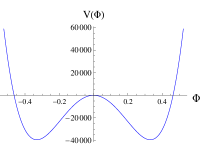
(a) Early times $(\tau_{0}\to 0)$

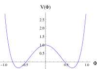
(b) Intermediate times $(\tau_{0}\sim\mathcal{O}(1))$

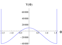
(c) Late times $(\tau_{0}>>1)$

Figure 2: The scalar potential on the constant $\tau$ slices, $\Sigma|_{\tau=\tau_{0}}$ (Eq. (22)), for early, intermediate and late times. We set $\kappa=\lambda=1$ and $\epsilon=0.9$. Notice the increased depth of the two degenerate minima in early and late times and the rise of the maxima in late times.

We conclude that most of the links of the slinky experience a fall from the two walls of $V(\Phi)$ (around $\Phi=\pm\pi/2$) towards the minima, the latter approaching the $\Phi=\pm\pi/2$ values as $\tau\to\infty$. Hence, it is only at late times that we can interpret the scalar profile in Eq. (18) as a true kink interpolating between the two (cusped) degenerate minima of $V(\Phi)$, as speculated in Sec. 2.

4 From Domain Wall to Brane cosmology

In this section we elaborate on what it is exactly that we are going to interpret as brane cosmology in the above setup.

Observing the time evolution of $\phi(\omega,\tau)$, we realize that when $\tau\to\infty$ we are naturally in a thin brane limit, where the brane is located at $\omega=0$. Inspired by the thin brane limit of maximally 4-symmetric domain wall configurations with non vanishing brane cosmological constant, $\Lambda_{b}$ [40], we recall the way in which this cosmological constant is matched. To be more specific the brane cosmological constant is due to the energy density of the bulk soliton when it is squeezed to the very same brane it generates at $\omega=0$, once the thin limit is taken.

4.1 Obtaining the brane cosmological constant in the thick RS case

As an instructive exercise, we review the results of [40] for a maximally 4-symmetric domain wall configuration which admits the RS model as its thin limit. The metric ansatz is:

$$ds^{2}=-dy^{2}+e^{2f(y)}\left[dt^{2}-d\vec{x}^{2}\right].$$ (23)

Considering again a minimally coupled scalar field $\varphi$ in the geometry described by the above equation, one writes the Einstein and Klein-Gordon equations, which are significantly simpler than the time dependent case and obtains the following solution:

$$\varphi=A\arctan[\tanh(\beta y/2)]\qquad V(\varphi)=A^{2}\beta^{2}/8-(A^{2}\beta^{2}/8)(1+\kappa A^{2}/3)\sin^{2}(2\varphi/A),$$ (24)

where $A$ and $\beta$ are constants. The geometry that corresponds to the above kink configuration and potential is dictated by $e^{f(y)}$, where:

$$e^{f(y)}=D[\cosh(\beta y)]^{-\kappa A^{2}/12}.$$ (25)

The thin limit of the above configuration is a delicate one in which $\beta\to\infty$, $A\to 0$ and $A^{2}\beta$ is fixed. In this limit $f\to-\kappa A^{2}\beta|y|/12$, such that $f^{\prime}\to-(\kappa A^{2}\beta/12)(\theta(y)-\theta(-y))$ and $f^{\prime\prime}\to-(\kappa A^{2}\beta/6)\delta(y)$. The resulting bulk geometry is that of a slice of $AdS_{5}$ divided by the brane (infinitely thin domain wall centered at $y=0$) into two disconnected regions, across which there is a jump of the extrinsic curvature. On identifying the degenerate minima of the potential in Eq. (24) with the 5D cosmological constant associated to the thin-limit $AdS_{5}$ space, one obtains:

$$V(\pm\pi A/4)=\Lambda_{5}=-\kappa A^{4}\beta^{2}/24\quad\Rightarrow\quad f^{\prime\prime}\to-2(-\Lambda_{5}\kappa/6)^{1/2}\delta(y).$$ (26)

The presence of the delta function in $f^{\prime\prime}$ combined with the (00) component of the Einstein equations for the metric in Eq. (23) [40], entail that both $\varphi^{\prime 2}$ and $V(\varphi)$ must contain the same delta function. Consequently, in the thin limit a term $e^{2f}[\varphi^{\prime 2}/2+V(\varphi)]\to A^{2}\beta/2\delta(y)=\Lambda_{b}\delta(y)$ is generated in $T_{00}$. This term corresponds to a brane cosmological constant, which automatically satisfies the RS fine tuning relation $\Lambda_{5}+\kappa\Lambda_{b}^{2}/6=0$. Namely, what had to be put by hand in the RS model is an output of the above dynamics.

An alternative way to derive $\Lambda_{b}$ is by requiring the 5D action $\int dy\sqrt{-g}\mathcal{L}=-\int dye^{4f}[\varphi^{\prime 2}/2$
$+V(\varphi)]=(3/\kappa)\int dye^{4f}(f^{\prime\prime}+2f^{\prime 2})$ to generate the RS action $\int dye^{4f}(-\Lambda_{5}-\Lambda_{b}\delta(y))$ in the thin limit. Using this prescription it is clear that $\Lambda_{5}$ comes only from the $2f^{\prime 2}$ term and $\Lambda_{b}$ comes only from the $f^{\prime\prime}$ term. The RS fine tuning relation is obviously satisfied by these results.

4.2 Obtaining the brane cosmological constant for slinky configurations

In our case we will assume that the time evolution of the kink configuration of Eq. (18), also controlled by the dimensionless parameter $\lambda$, is slow enough that a thin brane limit can be taken at every constant time slice, similarly to the maximally 4-symmetric case of [40]. Then, by matching to an instantaneous RS-like action or inspecting the behavior of $T_{00}$, we determine the bulk ($\Lambda_{5}(\tau)$) and brane induced ($\Lambda_{b}(\tau)$) cosmological constants at each slice of constant $\tau$. The brane (bulk) cosmological constant is an energy density which is constant in the instantaneous 3(4) space dimensions and satisfies $p=-\rho$.

To further elaborate along the lines of the above procedure, we first write the metric components along a constant $\tau$ slice, at say $\tau=\tau_{0}$:

$$\left.ds^{2}\right|_{\tau=\tau_{0}}=g^{\Sigma_{0}}_{ij}dx^{i}dx^{j}=-a^{2}(\omega,\tau=\tau_{0})d\vec{x}^{2}-\epsilon^{2}a^{2}(\omega,\tau=\tau_{0})d\omega^{2}=\frac{-1}{{1+\tilde{\lambda}^{2}\omega^{2}}}[d\vec{x}^{2}+\epsilon^{2}d\omega^{2}],$$ (27)

where $\tilde{\lambda}=\tau_{0}\lambda$ and spatial indices $i,j=x,y,z,\omega$. We note in passing that the metric ansatz we chose in Eq. (5) is conformally flat, but in contrast with the maximally 4-symmetric cases in [37, 38, 39, 40, 41], it does not admit an asymptotic $AdS_{5}$ limit (with a 5D cosmological constant corresponding to the value of the minima of the potential), due to the non-removable coordinate dependence in $V(\phi)$. Moreover, although we have written the time and extra dimension as $\tau$ and $\omega$, respectively, we recall that the $\tau-\omega$ symmetric ansatz for the warp factors in Eq. (17), is inspired by the solutions to the maximally 4-symmetric case with a conformal extra dimensional coordinate [46]. Thus, in order to inspect the cosmological time, $t$, and proper distance coordinate, $y$, we should in principle rewrite the solution using the relations $dy=b(\omega,\tau)d\omega$ and $dt=a(\omega,\tau)d\tau$ . Provided no singularity occurs in the coordinate transformation, we can work with $(\omega,\tau)$ coordinates and later transform to $(y,t)$ coordinates without loss of generality.

Considering the instantaneous geometry on each constant time slice described by the metric in Eq. (27), we obtain the bulk energy density and match it to a RS-like setup as follows. From the action in Eq. (4), or equivalently from the (00) component of the energy momentum tensor $T_{00}=(1/2)\dot{\phi}^{2}+(1/2\epsilon^{2})\phi^{\prime 2}+a^{2}V(\phi)$ (where $T_{MN}=(2/\sqrt{G})\delta\mathcal{L}/\delta G^{MN}$ and the Einstein Equations take the form $R_{MN}-(1/2)G_{MN}R=\kappa T_{MN}$), we realize that we have three separate contributions to the energy density which we label as: $\Omega_{\phi^{\prime 2}}$, $\Omega_{\dot{\phi}^{2}}$ and $\Omega_{V(\phi)}$, where $T_{00}=\Omega_{\phi^{\prime 2}}+\Omega_{\dot{\phi}^{2}}+\Omega_{V(\phi)}$ and

$$\Omega_{\phi^{\prime 2}}=\frac{1}{2\epsilon^{2}}\phi^{\prime 2}=\frac{3\tau^{2}\lambda^{2}}{2\kappa\epsilon^{2}(1+\lambda^{2}\omega^{2}\tau^{2})^{2}}=\frac{3\tilde{\lambda}^{2}}{2\kappa\epsilon^{2}(1+\tilde{\lambda}^{2}\omega^{2})^{2}},$$ (28)

$$\Omega_{\dot{\phi}^{2}}=\frac{1}{2}\dot{\phi}^{2}=\frac{3\omega^{2}\lambda^{2}}{2\kappa(1+\lambda^{2}\omega^{2}\tau^{2})^{2}}=\frac{3\omega^{2}\lambda^{2}}{2\kappa(1+\tilde{\lambda}^{2}\omega^{2})^{2}},$$ (29)

$$\Omega_{V(\phi)}=a^{2}V(\phi)=\frac{3\lambda^{2}\left(\tau^{2}-\omega^{2}\epsilon^{2}\right)\left(1-4\tau^{2}\omega^{2}\lambda^{2}\right)}{2k\epsilon^{2}\left(1+\tau^{2}\omega^{2}\lambda^{2}\right)^{2}}=\frac{3\left(\tilde{\lambda}^{2}-4\tilde{\lambda}^{4}\omega^{2}-\lambda^{2}\omega^{2}\epsilon^{2}+4\tilde{\lambda}^{2}\lambda^{2}\omega^{4}\epsilon^{2}\right)}{2k\epsilon^{2}\left(1+\tilde{\lambda}^{2}\omega^{2}\right)^{2}}.$$ (30)

In the above equations the second equality is written on $\Sigma|_{\tau=\tau_{0}}$, on which we are going to characterize each of the above contributions, term by term, to determine the localization properties of the associated energy densities and consequently what should be interpreted as $\Lambda_{b}(\tau_{0})$.

To implement the procedure described in the above paragraph, we perform a transformation $\omega\to y$ to a proper distance extra dimensional coordinate defined on each constant time slice, $\Sigma|_{\tau=\tau_{0}}$. Using Eq. (27) we obtain:

$$a(\omega,{\tau=\tau_{0}})d\omega=\frac{1}{\sqrt{1+\tilde{\lambda}^{2}\omega^{2}}}d\omega=dy\quad\Rightarrow\quad y={\rm arcsinh}(\tilde{\lambda}\omega)/\tilde{\lambda}\quad\Rightarrow\quad\omega=\sinh(\tilde{\lambda}y)/\tilde{\lambda}.$$ (31)

While the scaling of each term in the energy densities in Eqs. (28)-(30) with the time coordinate $\tau$ is determined by the powers of $\tilde{\lambda}$, their $\omega$ dependence remains explicit and is translated into the dependence on $y$ according to Eq. (31). The thin limit on each constant $\tau$ slice (when $\tau_{0}$ is simply a finite constant), is taken in principle by letting $\lambda\to\infty$. However, this limit is not well defined since the $\lambda$ dependence of all contributions is such that most of them will naively vanish in this limit. We can in principle overcome this problem by modifying $\phi$, $V(\phi)$ and $a(\omega,\tau=\tau_{0})$ to contain an additional pre-factor $A$ such that the thin limit is taken by keeping $A^{2}\lambda$ fixed while letting $A\to 0$ and $\lambda\to\infty$ as in [40]. However, such a modification of the warp factor, $a(\omega,\tau=\tau_{0})$, by virtue of Eqs. (11) and (12), will result in a non solitonic profile which blows towards infinity and will therefore fails to generate the thick brane (kink) we are looking for in the first place.

On the other hand, by simply observing the $\omega$ dependence of the same contributions in Eqs. (28)-(30), we see that they are all (except for the last term in Eq. (30)) peaked at (or around) $\omega=0(y=0)$. In particular, the common denominator for all contributions, $\tilde{D}(\tilde{\lambda},\omega)\equiv 1/(\sqrt{1+\tilde{\lambda}^{2}\omega^{2}})^{4}$ translates into $[sech(\tilde{\lambda}y)]^{4}$, which is strongly peaked at $y=0$ when $\tilde{\lambda}\to\infty$. Moreover, the $\omega$ dependence of $\Omega_{\phi^{\prime 2}}$, $\Omega_{\dot{\phi}^{2}}$ and $\Omega_{V(\phi)}$ is characterized by three distinct behaviours, $\tilde{D}$, $\omega^{2}\tilde{D}$ and $\omega^{4}\tilde{D}$, each of which also enters with different powers of $\tilde{\lambda}$. Since $\omega=\sinh(\tilde{\lambda}y)/\tilde{\lambda}$, it is clear that the $\omega^{2}\tilde{D}$ terms will also be peaked around $\omega=0$. So, a priori it seems like all of the energy densities in Eqs. (28)-(30) should be interpreted as contributions to the brane cosmological constant and do not correspond to any bulk cosmological constant, except for the fourth term in $\Omega_{V}$. In order to determine the brane induced cosmological constant we will integrate the densities of Eqs. (28)-(30) over $\omega$ on $\Sigma|_{\tau=\tau_{0}}$, to get a result which we are going to interpret as the instantaneous cosmological constant on the 3-brane located at $\omega=0$, at $\tau=\tau_{0}$. Labelling the four terms in $\Omega_{V}$ of Eq. (30) as $\Omega_{V}^{1,2,3,4}$, we realize that $\Omega_{\phi^{\prime 2}}=\Omega_{V}^{1}$ and $\Omega_{\dot{\phi}^{2}}=-\lambda^{2}\epsilon^{2}\Omega_{V}^{2}/(4\tilde{\lambda}^{4})=-\Omega_{V}^{3}$.

The limits of integration $\omega\to\pm\infty$ translate into $y\to\pm\infty$, as it can be inferred from Eq. (31). Starting from $\Omega_{\phi^{\prime 2}}$ and recalling that $d\omega=\cosh(\tilde{\lambda}y)dy$ we get:

$$\int d\omega\sqrt{G}\Omega_{\phi^{\prime 2}}=\int dy\frac{3\tilde{\lambda}^{2}}{2\kappa\epsilon(\cosh^{8}(\tilde{\lambda}y))}=\frac{3\tilde{\lambda}^{2}}{2\kappa\epsilon}\left(\left.\frac{16\tanh(\tilde{\lambda}y)}{35\tilde{\lambda}}\right|^{y_{+}\to+\infty}_{y_{-}\to-\infty}+\ldots\right)\approx\frac{48\tilde{\lambda}}{35\kappa\epsilon},$$ (32)

where the $\ldots$ stand for extra terms which are proportional in addition to $sech(\tilde{\lambda}y)^{2,4,6}$. These terms yield negligible contributions when the $y\to\pm\infty$ integration limits are taken. This will be especially true when the $\tilde{\lambda}\to\infty$ limit will be taken, a subtle case, which is treated separately with a different procedure in Sec. 4.3. Nevertheless, an explicit calculation of the integral in this limit will yield the same $\tilde{\lambda}$ (and $\epsilon$) scaling behavior with a different numerical pre-factor, which will correspond to the same late time cosmology on the brane.

Turning to $\Omega_{\dot{\phi}^{2}}$ and the related $\Omega_{V}^{2,3}$ we get:

$$\int d\omega\sqrt{G}\Omega_{\dot{\phi}^{2}}=\int dy\frac{3\lambda^{2}\epsilon}{2\kappa\tilde{\lambda}^{2}}\,\frac{\sinh^{2}(\tilde{\lambda}y)}{\cosh^{8}(\tilde{\lambda}y)}=\frac{3\lambda^{2}\epsilon}{2\kappa\tilde{\lambda}^{2}}\left(\left.\frac{8\tanh(\tilde{\lambda}y)}{105\tilde{\lambda}}\right|^{y_{+}\to+\infty}_{y_{-}\to-\infty}+...\right)\approx\frac{8\lambda^{2}\epsilon}{35\kappa\tilde{\lambda}^{3}},$$ (33)

which implies:

$$\int d\omega\sqrt{G}\Omega_{V}^{2}=-\frac{4\tilde{\lambda}^{4}}{\lambda^{2}\epsilon^{2}}\int d\omega\sqrt{G}\Omega_{\dot{\phi}^{2}}\approx-\frac{32\tilde{\lambda}}{35\kappa\epsilon}.$$ (34)

Finally, we turn to $\Omega_{V}^{4}$, which seems to have different localization properties from the other energy density contributions. After integration, we obtain:

$$\int d\omega\sqrt{G}\Omega_{V}^{4}=\frac{6\epsilon\lambda^{2}}{\kappa\tilde{\lambda}^{2}}\int\frac{\sinh^{4}(\tilde{\lambda}y)}{\cosh^{8}(\tilde{\lambda}y)}dy=\frac{6\epsilon\lambda^{2}}{\kappa\tilde{\lambda}^{2}}\left(\left.\frac{2\tanh(\tilde{\lambda}y)}{35\tilde{\lambda}}\right|^{y_{+}\to+\infty}_{y_{-}\to-\infty}+...\right)\approx\frac{24\lambda^{2}\epsilon}{35\kappa\tilde{\lambda}^{3}}.$$ (35)

Summarizing, we see that while the contributions of $\Omega_{V}^{3}$ and $\Omega_{\dot{\phi}^{2}}$ cancel each other, the identical contributions of $\Omega_{\phi^{\prime 2}}$ and $\Omega_{V}^{1}$ add up to yield an energy density peaked at $y=0$, and scales with $\tilde{\lambda}$. Together with the contribution coming from $\Omega_{V}^{2}$, this energy density is positive and amounts to $\Omega_{\tilde{\lambda}^{1}}^{brane}\simeq 64\tilde{\lambda}/(35\kappa\epsilon)$. As we shall show below the contribution coming from $\Omega_{V}^{4}$ corresponds instead to an instantaneous bulk energy density, which is a direct generalization of the bulk cosmological constant, $\Lambda_{5}$, of the maximally 4 symmetric case discussed in [40]. Further insight into the role of these energy densities will be gained through the procedure described in the next section.

4.3 The cosmological constant from matching to an instantaneous RS-like action

To get a better understanding of the localization properties of $\Omega_{V}^{1,2,3,4}$ and $\Omega_{\dot{\phi}^{2},\phi^{\prime 2}}$, in particular in their natural (yet problematic) late time thin limit, $\tilde{\lambda}\to\infty$, we first conveniently rewrite the equations of motion in terms of $f_{a}(\omega,\tau)$, defined as:

$$e^{f_{a}(\omega,\tau)}=a(\omega,\tau)\quad\Rightarrow\quad f_{a}(\omega,\tau)=-\ln(\sqrt{1+\lambda^{2}\omega^{2}\tau^{2}})\quad\Rightarrow\quad f_{a}(y,\tau)=-\ln\cosh(\tilde{\lambda}y),$$ (36)

where the last equality is written on a constant $\tau$ slice according to the coordinate transformation of Eq. (31). Since $b(\omega,\tau)=\epsilon a(\omega,\tau)$, we have $H(\omega,\tau)=F(\omega,\tau)=\dot{f_{a}}$ and $h(\omega,\tau)=f(\omega,\tau)=f_{a}^{\prime}$. Thus, it is straightforward to rewrite Eqs. (8), (11) and (12) in terms of $f_{a}(\omega,\tau)$ and its derivatives and subsequently use these equations to rewrite the action of Eq. (4) in terms of $f_{a}$. The resulting action acquires the following form:

$$S=\int d^{5}x\sqrt{G}\left(\frac{1}{2}a^{-2}\dot{\phi}^{2}-\frac{1}{2\epsilon^{2}}a^{-2}\phi^{\prime 2}-V(\phi)\right)=\int d^{5}x\sqrt{G}e^{-2f_{a}}\frac{3}{\kappa}\left(\frac{f_{a}^{\prime\prime}}{\epsilon^{2}}-\ddot{f_{a}}+\frac{f_{a}^{\prime 2}}{\epsilon^{2}}-\dot{f}_{a}^{2}\right).$$ (37)

The matching to an instantaneous RS-like action should be performed in the thin ($\tilde{\lambda}\to\infty$) limit of the domain wall configuration obtained in Sec. 2. On constant $\tau$ surfaces $\Sigma|_{\tau=\tau_{0}}$ the RS-like action will consist of a bulk cosmological constant term and a 3-brane cosmological constant, where the brane is located at $y=0$ (or $\omega=0$). To match we first transform the action of Eq. (37) to $y$ coordinates and require that:

$$S = (\int d\tau)\int d^{3}xd\omega\sqrt{G}e^{-2f_{a}(\omega,\tau)}\frac{3}{\kappa}\left(\frac{f_{a}^{\prime\prime}}{\epsilon^{2}}-\ddot{f_{a}}+\frac{f_{a}^{\prime 2}}{\epsilon^{2}}-\dot{f}_{a}^{2}\right)$$ (38)

$$= (\int d\tau)\int d^{3}xdy\sqrt{G}e^{-f_{a}(y,\tau)}\frac{3}{\kappa}\left(\frac{f_{a}^{\prime\prime}}{\epsilon^{2}}+2\frac{f_{a}^{\prime 2}}{\epsilon^{2}}-e^{-2f_{a}}(\ddot{f_{a}}-\dot{f}_{a}^{2})\right)$$

$$\,\,\underset{\tilde{\lambda}\to\infty}{\longrightarrow}\,\, (\int e^{f_{a}}d\tau)\left[\int dyd^{3}x\sqrt{g^{\Sigma_{0}}}(-\Lambda_{bulk})+\int d^{3}x\sqrt{g^{(3)}}(-\Lambda_{3-brane})\right]\,.$$

Using $\cosh(\tilde{\lambda}y)\underset{\tilde{\lambda}\to\infty}{\to}e^{\tilde{\lambda}|y|}/2$ we obtain all relevant quantities on $\Sigma|_{\tau=\tau_{0}}$, in the thin ($\tilde{\lambda}\to\infty$) limit.

$$f_{a}(y)\underset{\tilde{\lambda}\to\infty}{\to}-\tilde{\lambda}|y|\quad\Rightarrow\quad a(y)\underset{\tilde{\lambda}\to\infty}{\longrightarrow}2e^{-\tilde{\lambda}|y|},$$ (39)

$$f_{a}^{\prime}(y)\equiv\frac{df_{a}(y)}{dy}=-\tilde{\lambda}\tanh(\tilde{\lambda}y)\underset{\tilde{\lambda}\to\infty}{\longrightarrow}-\tilde{\lambda}(\theta(y)-\theta(-y)),$$ (40)

$$f_{a}^{\prime\prime}(y)\equiv\frac{d^{2}f_{a}(y)}{dy^{2}}=-\tilde{\lambda}^{2}{\rm sech}^{2}(\tilde{\lambda}y)\underset{\tilde{\lambda}\to\infty}{\longrightarrow}-2\tilde{\lambda}\delta(y).$$ (41)

We immediately realize that the $\tilde{\lambda}\to\infty$ limit of $f_{a}^{\prime\prime}(y)$ in Eq. (38), will generate a brane localized energy density proportional to $\tilde{\lambda}$, $\Lambda_{3-brane}^{f_{a}^{\prime\prime}}=6\tilde{\lambda}/(\kappa\epsilon)$, which agrees with the previous results obtained by analyzing the various terms in $T_{00}$ in Sec. 4.2. In particular the brane cosmological constant, $\Lambda_{3-brane}^{f_{a}^{\prime\prime}}$, is related to the contributions of the $\Omega_{\phi^{\prime 2}}$ and $\Omega_{V}^{2}$ densities of Eqs. (28) and (30) by:

$$\Omega_{\phi^{{}^{\prime}2}}+\Omega_{V}^{1}\underset{\tilde{\lambda}\to\infty}{\longrightarrow}T_{00}(\Lambda_{3-brane}^{f_{a}^{\prime\prime}})=e^{2f_{a}}\delta(y)\Lambda_{3-brane}^{f_{a}^{\prime\prime}}$$ (42)

The contribution coming from $f_{a}^{\prime 2}(y)$ will instead correspond to the aforementioned generalization of the bulk cosmological constant, $\Lambda_{5}$, appearing in [40] and Sec.4.1. These contributions are $y$ independent in the $\tilde{\lambda}\to\infty$ limit and will be specified later. To obtain the explicit form for the $\dot{f}_{a}$ and $\ddot{f}_{a}$ terms we act with derivatives with respect to $\tau$ on $f_{a}(\omega,\tau)$, since the coordinate transformation of Eq. (31) is defined only on constant $\tau$ surfaces. Once the derivatives have been obtained we express them in terms of $y$ on $\Sigma|_{\tau=\tau_{0}}$ which results in:

$$\dot{f}_{a}\equiv\frac{df_{a}(\omega,\tau)}{d\tau}|_{\Sigma|_{\tau=\tau_{0}}}=-\frac{\lambda\tilde{\lambda}\omega^{2}}{1+{\tilde{\lambda}}^{2}\omega^{2}}=-\frac{\lambda\sinh^{2}(\tilde{\lambda}y)}{\tilde{\lambda}\cosh^{2}(\tilde{\lambda}y)}\underset{\tilde{\lambda}\to\infty}{\longrightarrow}-\frac{\lambda}{\tilde{\lambda}}\left(\theta(y)-\theta(-y)\right)^{2}=-\frac{\lambda}{\tilde{\lambda}}\,.$$ (43)

This contribution also corresponds to a $y$ independent (totally delocalized in $y$) energy density in the $\tilde{\lambda}\to\infty$ limit. Finally, we inspect the $\tilde{\lambda}\to\infty$ limit of $\ddot{f}_{a}$ in an analogous way to $\dot{f}_{a}$ and obtain:

$$\ddot{f}_{a}\equiv\frac{d^{2}f_{a}(\omega,\tau)}{d\tau^{2}}|_{\Sigma|_{\tau=\tau_{0}}}=\frac{2{\tilde{\lambda}}^{2}\lambda^{2}\omega^{4}}{(1+{\tilde{\lambda}}^{2}\omega^{2})^{2}}-\frac{\lambda^{2}\omega^{2}}{1+{\tilde{\lambda}}^{2}\omega^{2}} = \frac{\lambda^{2}}{\tilde{\lambda}^{2}}\left(2\tanh^{4}(\tilde{\lambda}y)-\tanh^{2}(\tilde{\lambda}y)\right)$$

$$\underset{\tilde{\lambda}\to\infty}{\longrightarrow}\frac{\lambda^{2}}{\tilde{\lambda}^{2}}\left(2(\theta(y)-\theta(-y))^{4}-(\theta(y)-\theta(-y))^{2}\right)=\frac{\lambda^{2}}{\tilde{\lambda}^{2}}$$ (44)

From Eqs. (38), (43) and (44) we realize that the $\tanh(\tilde{\lambda}y)^{4}$ terms in $\dot{f_{a}}^{2}$ and $\ddot{f}_{a}$ are added to each other, leaving us with both $\tanh^{2}(\tilde{\lambda}y)$ and $\tanh^{4}(\tilde{\lambda}y)$ terms, which will together contribute to a $y$ dependent bulk energy density. Their contribution enters with a conformal prefactor $e^{-2f_{a}}$, implying that the associated bulk energy density, $\Omega_{\dot{f}_{a}^{2},\ddot{f}_{a}}$ behaves as $\cosh^{2}(\tilde{\lambda}y)\tanh(\tilde{\lambda}y)^{(2,4)}$. However, since the metric is strongly peaked at $y=0$ in the $\tilde{\lambda}\to\infty$ limit and we care about the contribution of $\Omega_{\dot{f}_{a}^{2},\ddot{f}_{a}}$ to the induced instantaneous brane cosmological constant, the $e^{-2f_{a}}$ conformal prefactor does not modify the step function limits of Eqs. (43) and (44) relevant for our purpose. Notice also that if we integrate over $y$, the total contribution of these energy densities remains finite. The associated bulk contribution to the brane induced cosmological constant amounts to $\Lambda_{bulk}^{\dot{f}_{a},\ddot{f}_{a}}=(6/\kappa)\lambda^{2}/\tilde{\lambda}^{2}$ in the $\tilde{\lambda}\to\infty$ limit. This result corresponds to the contribution of $\Omega_{V}^{4}=(6/\kappa)(\lambda^{2}/\tilde{\lambda}^{2})\tanh^{4}(\tilde{\lambda}y)$ in Eq. (30).

Finally, from Eqs. (38) and (40) the contribution of the $f_{a}^{\prime 2}$ term to the bulk energy density (on $\Sigma_{\tau=\tau_{0}}$), $\Lambda^{f_{a}^{\prime}}_{bulk}=-(6/\kappa)\tilde{\lambda}^{2}/\epsilon^{2}$ corresponds to the contribution of $\Omega_{V}^{2}$, which is thus interpreted as a bulk energy term.

5 Simplest Cosmological scenarios

The above analysis tells us that in the thin ($\tilde{\lambda}\to\infty$) limit the slinky configuration introduced in Sec. 2 is equivalent to a brane in a $AdS_{5}$-like bulk characterized by the warp factor $a(y)=e^{-\tilde{\lambda}|y|}$. We have found that the bulk and brane cosmological constants are given by:

$$\Lambda_{5}^{sl.}=\frac{6}{\kappa}\left(\frac{\lambda^{2}}{\tilde{\lambda}^{2}}-\frac{\tilde{\lambda}^{2}}{\epsilon^{2}}\right)\qquad\Lambda_{b}^{sl.}=\frac{6}{\kappa}\frac{\tilde{\lambda}}{\epsilon}.$$ (45)

From the above equation, we immediately realize that the RS fine tuning relation is asymptotically satisfied on every constant $\tau$ slice, in the limit $\tilde{\lambda}\to\infty$ (;large times) thus supplementing us with a static brane. This happens for any value of the parameter $\epsilon$. Also notice that, unlike the solution in [46], $\epsilon=1$ does not correspond to a free solution. At any finite $\tilde{\lambda}$, we have an induced brane dark energy density given by:

$$(\Lambda_{b}^{ind.})_{slinky}=\kappa\frac{(\Lambda_{b}^{sl.})^{2}}{6}+\Lambda_{5}^{sl.}=\frac{6\tilde{\lambda}^{2}}{\kappa}\left(\frac{1}{\epsilon^{2}}-\frac{1}{\epsilon^{2}}\right)+\frac{6\lambda^{2}}{\kappa\tilde{\lambda}^{2}}=\frac{6\lambda^{2}}{\kappa\tilde{\lambda}^{2}}\,.$$ (46)

Notice that the brane cosmological constant, $\Lambda_{b}^{sl.}$ enters quadratically in the RS fine tuning relation. This is in exact correspondence to the well known analysis of fundamental brane cosmology by Deffayet et al. [18, 22], as follows. In the general time-dependent fundamental brane case, one solves the 5-dimensional Einstein equations by imposing the Israel matching conditions relating the discontinuities in the derivatives of the metric components across $y=0$, to delta distribution sources (see [18]). It turns out that the behaviors of the brane sources and the metric components evaluated at $y=0$ are independent of the metric solutions in the bulk, and obey a modified Friedmann equation where the brane energy density enters quadratically.

Thus, the late time (large $\tilde{\lambda}$) cosmology of the simplest slinky configuration reported in Sec. 2, in the absence of additional sources, is simply driven by a dark energy density $(\Lambda_{b}^{ind.})_{slinky}$, which will consist only of the bulk contributions generated by the $\dot{f}_{a}^{2}$ and $\ddot{f}_{a}$ terms in the action of Eq. (38), which decay like $1/\tau^{2}$ for large values of $\tau$.

To conclude the analysis of the late time ($\tau>>1$) cosmology on the brane we write (and solve) the effective Friedmann equation for the evolution of the scale factor of the instantaneous 3-brane:

$$H_{b}(\tau)^{2}=\kappa\Lambda_{b}^{ind.}=\frac{6}{\tau^{2}}\Rightarrow a_{b}(\tau)=e^{\int H_{b}(\tau)d\tau}=C_{b}\,\tau^{\sqrt{6}},$$ (47)

where $H_{b}(\tau)$ is the brane Hubble constant and $C_{b}$ is an integration constant. Thus, the late time brane is accelerating with a power law for the scale factor, corresponding to a deceleration parameter, $q=-a_{b}\,\ddot{a_{b}}/\dot{a}_{b}^{2}=1/\sqrt{6}-1\simeq-0.6$, which is rather plausible if we simply treat $\tau$ as the cosmological time.

The addition of (a-priori) brane localized sources (matter, radiation), will obviously enable various modifications of the brane cosmological evolution, all of which will be analogous to the analysis of [18, 22]. Needless to say, the latter possibility is highly implausible due to the large element of arbitrariness or the lack of underlying dynamics.

Finally, we comment on the early time cosmological interpretation of the solution reported in Sec. 2. Since at early times ($\tilde{\lambda}\to 0$) the kink configuration and warp factor are nearly flat ($\phi\to 0$ and $a(\omega,\tau)\to 1$), we should expect that the average of the large early time bulk energy densities, $\Omega_{\dot{f}_{a},\ddot{f}_{a}}$, will dictate the cosmological evolution of the 4D geometry obtained by integrating out $\omega$ (or $y$).

The main problem with this early time picture is the absence of a brane, or a specific region in the extra dimension, corresponding to the 4D DW brane universe we wish to obtain in the first place. It is at this point that we take advantage of the fact that the solution reported in Sec. 2 is symmetric in $\omega$ and $\tau$. By performing the same analysis of Sec. 4.3 on constant $\omega$ slices, $\Sigma|_{\omega=\omega_{0}}$, we realize that in the limit $\omega\to\infty$ the scalar field, $\phi$, becomes a “brane in time” ($\tau$-brane) localized at $\tau=0$. Similarly, the $\ddot{f}_{a}$ term in the action (Eq. (37)), will become a delta distribution in time for $\omega\to\infty$ , in analogy with Eq. (41) and will thus correspond to a brane localized energy density.

Given the above, the hypersurface $\Sigma|_{\tau=0}$ will correspond to the center of a thick “$\tau$-brane”, with a brane localized energy density that diverges as $\omega\to\infty$ - thus providing an element of creation, which occurs smoothly for any finite value of $\omega$, in the spirit of the Hartle-Hawking no boundary proposal.

To conclude, we find the cosmological interpretation of the slinky solution introduced in Sec. 2 and studied above to be plausible and problematic at the same time. It is plausible, because an extremely simple 5D setup with a single scalar field is able to generate a DW brane universe with an early and late time accelerating phases, thus addressing directly the dark energy paradigm.

The main problem with the same interpretation stems from the subtle identification of early time dynamics and the interpolation between the late time and early time regimes. The most natural explanation, which seems to suggest itself, is that our DW brane universe is localized towards $\omega\to\infty$ as $\tau\to 0$ (which can also be perceived as its creation at this point in the extra dimension) and evolves to an infinitely thin brane at $\omega=0$ for $\tau\to\infty$, thus corresponding to a different (non trivial) watershed than the one we naively started with, namely the line $\omega=0$. To realize such a possibility one must find a new solution in the intermediate time regime, which is able to interpolate between the above early and late time behaviors. Simultaneously, this interpolating solution should satisfy the $(05)$ constraint (Eq. (10)), to balance the DW-bulk energy transfer in intermediate times (Eq. (21)). Further study of this possibility and the search for alternative solutions will be the subject of future publications.

6 Conclusions

In this paper we have proposed a novel type of time dependent DW configurations in a warped 5D space time. The purpose is to find a dynamical realization for braneworld cosmology. After discussing the initial symmetry of the time $t$ and some extra spatial dimension $y$ prior to the dynamics generating the DW brane universe, we have introduced the notion of slinky configurations. We require that such configurations satisfy the most obvious properties for a cosmologically plausible time dependent DW brane setup, namely an element of creation, a finite inflationary period and late time acceleration.

The simplest configuration we were able to find was based on a time “proportional” ansatz for the metric warp factors, corresponding to a conformally flat 5D metric. This configuration has most of the desired features, however it introduces an explicitly coordinate dependent scalar potential. As part of future steps in this direction, it will be important to clarify the role and implications of properties such as non factorizability in $(t,y)$ of the solutions and how these properties are related to the possible loss of 5D covariance.

The cosmological evolution of the proposed DW brane configuration was studied by constructing instantaneous energy densities associated with the DW scalar and its supporting potential on constant time ($\tau$) slices, where the potential can be written in a covariant form. This procedure allowed to identify bulk and brane induced energy densities (cosmological constants). The resulting cosmology was shown to include a smooth element of creation (in the spirit of the Hartle-Hawking no boundary proposal [52]), a naturally terminating inflationary period and a late time acceleration phase.

An underlying dynamics that accounts for more detailed cosmological features would in principle require the addition of matter and gauge fields, rendering the problem even more difficult to solve. No satisfactory solution has been found up to date. Another, simplifying avenue is to study cosmological perturbations on a given slinky configuration. We plan to search for new more satisfactory solutions in the context of slinky configurations and follow the proposed avenues in order to probe their cosmological implications.

The long term purpose of this study is to find a cosmologically plausible and fully dynamical DW brane setup, which unifies cosmological and particle physics aspects, and can be used for particle physics in the spirit of [47]. A configuration able to satisfy simultaneously the constraints coming from both cosmological observations and collider physics experiments is certainly highly desirable; it is also appealing the possibility that its building blocks require nothing more than General Relativity and Quantum Field Theory in 5D.

References

- [1] T. Kaluza, “On the Problem of Unity in Physics,” Sitzungsber.Preuss.Akad.Wiss.Berlin (Math.Phys.) 1921 (1921) 966–972. Often incorrectly cited as Sitzungsber.Preuss.Akad.Wiss.Berlin (Math. Phys.) K1,966. In reality there is no volume number, so SPIRES used the year in place of a volume number.
- [2] O. Klein, “Quantum Theory and Five-Dimensional Theory of Relativity. (In German and English),” Z.Phys. 37 (1926) 895–906.
- [3] P. Horava and E. Witten, “Eleven-Dimensional Supergravity on a Manifold with Boundary,” Nucl. Phys. B475 (1996) 94–114, hep-th/9603142.
- [4] P. Horava and E. Witten, “Heterotic and type I string dynamics from eleven dimensions,” Nucl. Phys. B460 (1996) 506–524, hep-th/9510209.
- [5] N. Arkani-Hamed, S. Dimopoulos, and G. Dvali, “The Hierarchy problem and new dimensions at a millimeter,” Phys.Lett. B429 (1998) 263–272, hep-ph/9803315.
- [6] I. Antoniadis, “A Possible new dimension at a few TeV,” Phys.Lett. B246 (1990) 377–384.
- [7] I. Antoniadis, N. Arkani-Hamed, S. Dimopoulos, and G. Dvali, “New dimensions at a millimeter to a Fermi and superstrings at a TeV,” Phys.Lett. B436 (1998) 257–263, hep-ph/9804398.
- [8] D. Kapner, T. Cook, E. Adelberger, J. Gundlach, B. R. Heckel, et. al., “Tests of the gravitational inverse-square law below the dark-energy length scale,” Phys.Rev.Lett. 98 (2007) 021101, hep-ph/0611184.
- [9] A. A. Geraci, S. J. Smullin, D. M. Weld, J. Chiaverini, and A. Kapitulnik, “Improved constraints on non-Newtonian forces at 10 microns,” Phys.Rev. D78 (2008) 022002, 0802.2350.
- [10] A. Sushkov, W. Kim, D. Dalvit, and S. Lamoreaux, “New Experimental Limits on Non-Newtonian Forces in the Micrometer Range,” Phys.Rev.Lett. 107 (2011) 171101.
- [11] L. Randall and R. Sundrum, “A large mass hierarchy from a small extra dimension,” Phys. Rev. Lett. 83 (1999) 3370–3373, hep-ph/9905221.
- [12] L. Randall and R. Sundrum, “An alternative to compactification,” Phys. Rev. Lett. 83 (1999) 4690–4693, hep-th/9906064.
- [13] M. Visser, “An Exotic Class of Kaluza-Klein Models,” Phys.Lett. B159 (1985) 22, hep-th/9910093.
- [14] G. Gibbons and D. Wiltshire, “Space-Time as a Membrane in Higher Dimensions,” Nucl.Phys. B287 (1987) 717, hep-th/0109093.
- [15] K. Agashe, G. Perez, and A. Soni, “Flavor structure of warped extra dimension models,” Phys.Rev. D71 (2005) 016002, hep-ph/0408134.
- [16] M. S. Carena, A. Delgado, E. Ponton, T. M. Tait, and C. Wagner, “Precision electroweak data and unification of couplings in warped extra dimensions,” Phys.Rev. D68 (2003) 035010, hep-ph/0305188.
- [17] P. Brax, C. van de Bruck, and A.-C. Davis, “Brane world cosmology,” Rept.Prog.Phys. 67 (2004) 2183–2232, hep-th/0404011.
- [18] P. Binetruy, C. Deffayet, and D. Langlois, “Nonconventional cosmology from a brane universe,” Nucl.Phys. B565 (2000) 269–287, hep-th/9905012.
- [19] C. Csaki, M. Graesser, C. F. Kolda, and J. Terning, “Cosmology of one extra dimension with localized gravity,” Phys.Lett. B462 (1999) 34–40, hep-ph/9906513.
- [20] J. M. Cline, C. Grojean, and G. Servant, “Cosmological expansion in the presence of extra dimensions,” Phys.Rev.Lett. 83 (1999) 4245, hep-ph/9906523.
- [21] D. J. Chung and K. Freese, “Cosmological challenges in theories with extra dimensions and remarks on the horizon problem,” Phys.Rev. D61 (2000) 023511, hep-ph/9906542.
- [22] P. Binetruy, C. Deffayet, U. Ellwanger, and D. Langlois, “Brane cosmological evolution in a bulk with cosmological constant,” Phys.Lett. B477 (2000) 285–291, hep-th/9910219.
- [23] E. E. Flanagan, S. Tye, and I. Wasserman, “Cosmological expansion in the Randall-Sundrum brane world scenario,” Phys.Rev. D62 (2000) 044039, hep-ph/9910498.
- [24] G. Dvali and S. Tye, “Brane inflation,” Phys.Lett. B450 (1999) 72–82, hep-ph/9812483.
- [25] J. Khoury, B. A. Ovrut, P. J. Steinhardt, and N. Turok, “The Ekpyrotic universe: Colliding branes and the origin of the hot big bang,” Phys.Rev. D64 (2001) 123522, hep-th/0103239.
- [26] Y.-i. Takamizu and K.-i. Maeda, “Collision of domain walls and reheating of the brane universe,” Phys.Rev. D70 (2004) 123514, hep-th/0406235.
- [27] D. Baumann, A. Dymarsky, I. R. Klebanov, and L. McAllister, “Towards an Explicit Model of D-brane Inflation,” JCAP 0801 (2008) 024, 0706.0360.
- [28] C. S. Chan, P. L. Paul, and H. L. Verlinde, “A Note on warped string compactification,” Nucl.Phys. B581 (2000) 156–164, hep-th/0003236.
- [29] B. L. Altshuler, “String theory provides landmarks fixing RS branes’ positions: Possibility to deduce large mass hierarchy from small numbers,” hep-th/0511271.
- [30] B. S. Acharya, F. Benini, and R. Valandro, “Warped models in string theory,” hep-th/0612192.
- [31] P. Kanti, I. I. Kogan, K. A. Olive, and M. Pospelov, “Cosmological three-brane solutions,” Phys.Lett. B468 (1999) 31–39, hep-ph/9909481.
- [32] P. Mounaix and D. Langlois, “Cosmological equations for a thick brane,” Phys.Rev. D65 (2002) 103523, gr-qc/0202089.
- [33] I. Navarro and J. Santiago, “Unconventional cosmology on the (thick) brane,” JCAP 0603 (2006) 015, hep-th/0505156.
- [34] M. Cvetic and M. Robnik, “Gravity Trapping on a Finite Thickness Domain Wall: An Analytic Study,” Phys.Rev. D77 (2008) 124003, 0801.0801.
- [35] V. Rubakov and M. Shaposhnikov, “Do We Live Inside a Domain Wall?,” Phys.Lett. B125 (1983) 136–138.
- [36] K. Akama, “An Early Proposal of ’Brane World’,” Lect.Notes Phys. 176 (1982) 267–271, hep-th/0001113.
- [37] O. DeWolfe, D. Freedman, S. Gubser, and A. Karch, “Modeling the fifth-dimension with scalars and gravity,” Phys.Rev. D62 (2000) 046008, hep-th/9909134.
- [38] M. Gremm, “Four-dimensional gravity on a thick domain wall,” Phys.Lett. B478 (2000) 434–438, hep-th/9912060.
- [39] M. Gremm, “Thick domain walls and singular spaces,” Phys.Rev. D62 (2000) 044017, hep-th/0002040.
- [40] A. Davidson and P. D. Mannheim, “Dynamical localization of gravity,” hep-th/0009064.
- [41] M. Giovannini, “Gauge invariant fluctuations of scalar branes,” Phys.Rev. D64 (2001) 064023, hep-th/0106041.
- [42] C. Csaki, J. Erlich, T. J. Hollowood, and Y. Shirman, “Universal aspects of gravity localized on thick branes,” Nucl.Phys. B581 (2000) 309–338, hep-th/0001033.
- [43] A. Kehagias and K. Tamvakis, “Localized gravitons, gauge bosons and chiral fermions in smooth spaces generated by a bounce,” Phys.Lett. B504 (2001) 38–46, hep-th/0010112.
- [44] D. Bazeia, A. Gomes, and L. Losano, “Gravity localization on thick branes: A Numerical approach,” Int.J.Mod.Phys. A24 (2009) 1135–1160, 0708.3530.
- [45] T. R. Slatyer and R. R. Volkas, “Cosmology and fermion confinement in a scalar-field-generated domain wall brane in five dimensions,” JHEP 0704 (2007) 062, hep-ph/0609003. 29 pages, 12 figures/ minor changes, accepted by JHEP.
- [46] M. Giovannini, “Time-dependent gravitating solitons in five dimensional warped space-times,” Phys.Rev. D76 (2007) 124017, 0708.1830.
- [47] D. P. George, M. Trodden, and R. R. Volkas, “Extra-dimensional cosmology with domain-wall branes,” JHEP 0902 (2009) 035, 0810.3746.
- [48] R. Davies, D. P. George, and R. R. Volkas, “The Standard model on a domain-wall brane,” Phys.Rev. D77 (2008) 124038, 0705.1584.
- [49] A. Davidson, D. P. George, A. Kobakhidze, R. R. Volkas, and K. C. Wali, “SU(5) grand unification on a domain-wall brane from an E(6)-invariant action,” Phys.Rev. D77 (2008) 085031, 0710.3432.
- [50] V. Dzhunushaliev, V. Folomeev, and M. Minamitsuji, “Thick brane solutions,” Rept.Prog.Phys. 73 (2010) 066901, 0904.1775.
- [51] A. Davidson, D. Karasik, and Y. Lederer, “Geodesic nucleation and evolution of a de Sitter brane,” Phys.Rev. D72 (2005) 064011, gr-qc/0509127.
- [52] J. Hartle and S. Hawking, “Wave Function of the Universe,” Phys.Rev. D28 (1983) 2960–2975.
- [53] WMAP Collaboration, E. Komatsu et. al., “Seven-Year Wilkinson Microwave Anisotropy Probe (WMAP) Observations: Cosmological Interpretation,” Astrophys. J. Suppl. 192 (2011) 18, 1001.4538.