Kinetic derivation of a Hamilton-Jacobi traffic flow model

Abstract

Kinetic models for vehicular traffic are reviewed and considered from the point of view of deriving macroscopic equations. A derivation of the associated macroscopic traffic flow equations leads to different types of equations: in certain situations modified Aw-Rascle equations are obtained. On the other hand, for several choices of kinetic parameters new Hamilton-Jacobi type traffic equations are found. Associated microscopic models are discussed and numerical experiments are presented discussing several situations for highway traffic and comparing the different models.

1 Introduction

Macroscopic models for vehicular traffic have been first introduced by Lighthill and Whitham [23]. These models are based on the continuity equation for the density $\rho$ closing the equation by an equilibrium assumption on the mean velocity $u$, where $u$ is approximated by a uniquely determined equilibrium value, [23]. An additional momentum equation for $u$ has been introduced by Payne and Whitham in [19, 23] in analogy to fluid dynamics. To avoid certain inconsistencies, like wrong way traffic, of models such as the Payne/Whitham model a new macroscopic model has been introduced by Aw and Rascle [3], see also [1] or [10]. These models have been subsequently improved, for example, in [6, 7].

Kinetic equations for vehicular traffic can be found, for example, in [20, 18, 17, 14, 13]. Procedures to derive macroscopic traffic equations including the Aw/Rascle model from underlying kinetic models have been performed in different ways by several authors, see, for example, [11] and [16]. These procedures are developed in analogy to the transition from the kinetic theory of gases to continuum gas dynamics.

In the present paper these derivations are reviewed. A closer analysis shows that Aw-Rascle type traffic equations can be derived from kinetic problems for certain choices of kinetic parameters. For other choices, however, new equations with Hamilton-Jacobi terms are derived.

The paper is arranged in the following way: In Section 2 different reduced kinetic models are presented. Section 3 contains the derivation of the macroscopic models mentioned above. Section 4 contains the associated microscopic traffic flow models. Finally, in Section 5 numerical results are given comparing the derived macroscopic equations for several nonhomogeneous traffic flow situation.

2 Kinetic Models

The kinetic models presented in this section are based on work in [15, 13] and describe highway traffic in a cumulative way averaging over all lanes. These models are given by integro-differential and Fokker-Planck type equations respectively. In particular, the Fokker-Planck type models are changed allowing only for densities below a maximal density and for a better comparison of the models.

2.1 Correlations and the reduced density

The basic quantity in a kinetic approach is the single car distribution $f(x,v)$ describing the (number) density of cars at $x$ with velocity $v$. The total density $\rho$ on the highway is defined by

$$\rho(x)\;=\;\int_{0}^{w}f(x,v)dv,$$

where $w$ denotes the maximal velocity. Let $F(x,v)$ denote the probability distribution in $v$ of cars at $x$, i.e. $f(x,v)=\rho(x)F(x,v)$. Then , the mean velocity is

$$u(x)\;=\;\int_{0}^{w}vF(x,v)dv.$$

An important role is played by the distribution $f^{(2)}(x,v,h,v_{+})$ of pairs of cars being at the spatial point $x$ with velocity $v$ and leading cars at $x+h$ with velocity $v_{+}$. This distribution function has to be approximated by the one-vehicle distribution function $f(x,v)$. Usually, a chaos assumption is used,

$$f^{(2)}(x,v,h,v_{+})=q(h,v;f)\,f(x,v)\,F(x+h,v_{+}),$$

compare Nelson [17]. For a vehicle with velocity $v$ the function $q(h,v;f)$ denotes the distribution of leading vehicles with distance $h$ under the assumption that the velocities of the vehicles are distributed according to the distribution function $f$.

Moreover, we introduce thresholds for braking ($H_{B}$) and acceleration ($H_{A}$):

$$H_{X}=H_{X}(v)\;=\;H_{0}+vT_{X},\quad X=B,A.$$

$T_{B}<T_{A}$ are reaction times. $H_{0}$ denotes the minimal distance between the vehicles. For simplicity we choose $H_{A}$ and $H_{B}$ in the following as constants.

The distribution of leading vehicles $q(h,v;f)$ is prescribed a priori. The main properties, which $q(h,v;f)$ has to fulfill are positivity,

$$\int_{0}^{\infty}q(h,v;f)dh\;=\;1,$$

and

$$\int_{0}^{w}\int_{0}^{\infty}hq(h,v;f)dh\,F(v)dv\;=\;\frac{1}{\rho}.$$ (2.1)

Equation (2.1) means that the average headway of the cars is $1/\rho$. Here, the leading vehicles are assumed to be distributed in an uncorrelated way with a minimal distance $H_{B}$ from the car under consideration, see Nelson [17]:

$$q(h,v;f)\;=\;q(h;\rho)=\tilde{\rho}\,e^{-\tilde{\rho}(h-H_{B})}\,\chi_{[H_{B},\infty)}(h).$$

The reduced density $\tilde{\rho}$ has to be defined in such a way, that (2.1) is fulfilled. One obtains

$$\tilde{\rho}\;=\;\frac{\rho}{1-\rho\,\int_{0}^{w}H_{B}F(v)dv}\;=\;\frac{\rho}{1-\rho\,H_{B}}.$$ (2.2)

Remark 2.1

The reduced density $\tilde{\rho}$ must be positive, i.e.

$$\rho\;\;<\;\frac{1}{H_{B}}$$

We note that

$$q(H_{A};\rho)\;=\;\tilde{\rho}\,e^{-\tilde{\rho}(H_{A}-H_{B})}$$

and

$$q(H_{B};\rho)\;\;=\;\tilde{\rho}\;.$$

Moreover, from phenomenological considerations the probability of braking can be derived as

$$P_{B}=1-(1-\rho H_{B})e^{-\tilde{\rho}H_{B}},$$

see [9]. These basic considerations can be used to develop different kinetic models.

2.2 Models based on Integro-differential equations

A first kinetic model is derived using classical Boltzmann arguments. It is given by the following evolution equation for the distribution function $f$, see [16, 9]:

$$\partial_{t}f+v\partial_{x}f = C^{+}(f)$$

$$= \left[q_{B}P_{B}(G^{+}_{B}-L^{+}_{B})(f)+q_{A}(G^{+}_{A}-L^{+}_{A})(f)\right]$$

with

$$G_{B}^{+}(f) = \int\int_{\hat{v}>\hat{v}_{+}}|\hat{v}-\hat{v}_{+}|\sigma_{B}(v;\hat{v},\hat{v}_{+})f(x,\hat{v})F(x+H_{B},\hat{v}_{+})d\hat{v}d\hat{v}_{+}$$

$$L_{B}^{+}(f) = \int_{\hat{v}_{+}<v}|v-\hat{v}_{+}|f(x,v)F(x+H_{B},\hat{v}_{+})d\hat{v}_{+}$$

$$G_{A}^{+}(f) = \int\int_{\hat{v}<\hat{v}_{+}}|\hat{v}-\hat{v}_{+}|\sigma_{A}(v;\hat{v},\hat{v}_{+})f(x,\hat{v})F(x+H_{A},\hat{v}_{+})d\hat{v}d\hat{v}_{+}$$

$$L_{A}^{+}(f) = \int_{\hat{v}_{+}>v}|v-\hat{v}_{+}|f(x,v)F(x+H_{A},\hat{v}_{+})d\hat{v}_{+}$$

$G_{B},L_{B}$ stand for gain and loss terms resulting from braking interactions, $G_{A},L_{A}$ result from accelerating interactions. Reaching the braking line the vehicle brakes, such that the new velocity $v$ is distributed with a distribution function $\sigma_{B}$ depending on the old velocities $\hat{v},\hat{v}_{+}$. For acceleration, the new velocity is distributed according to $\sigma_{A}$.

Remark 2.2

In [9] additionally a relaxation term is introduced, describing a random behaviour of the drivers. It is given by

$$G_{S}(f)-L_{S}(f)\;=\;\nu(\int_{0}^{w}\sigma_{S}(v,\hat{v})f(x,\hat{v})d\hat{v}-f(v)).$$

This term is necessary as long as one is interested in a more detailed investigation of the stationary solutions of the kinetic model and the resulting fundamental diagrams. However, in the present investigation we aim at deriving different macroscopic equations without relaxation terms on the right hand side. For such a derivation it is sufficient to consider the simplified version above. For further remarks on this Boltzmann/Enskog approach to traffic flow modelling see [16].

Example 1

For the probability distributions $\sigma_{A},\sigma_{B}$ we choose the following simple expressions, see [9]:

$$\sigma_{B}(v,\hat{v},\hat{v}_{+})\;=\;\frac{1}{\hat{v}-\hat{v}_{+}}\,\chi_{[\hat{v}_{+},\hat{v}]}(v)$$ (2.4)

and

$$\sigma_{A}(v,\hat{v},\hat{v}_{+})\;=\;\frac{1}{\hat{v}_{+}-\hat{v}}\,\chi_{[\hat{v},\hat{v}_{+}]}(v).$$ (2.5)

This means we have an equidistribution of the new velocities between the velocity of the car and the velocity of its leading car.

Example 2

Another possible choice is, see [16]

$$\sigma_{B}(v,\hat{v})=\frac{1}{\hat{v}(1-\beta)}\chi_{[\beta\hat{v},\hat{v}]}(v)$$

and

$$\sigma_{A}(v,\hat{v})=\frac{1}{\mbox{min}(w,\alpha\hat{v})-\hat{v}}\chi_{[\hat{v},\mbox{min}(w,\alpha\hat{v})]}(v).$$

2.3 Models based on Vlasov-Fokker-Planck equations

In [13] a kinetic model based on a VlasovFokker-Planck approach has been developed:

$$\partial_{t}f+v\partial_{x}f=C^{+}(f)=-\partial_{v}\big{(}B[f]f\big{)}.$$ (2.6)

Here, $f$ stands again for a traffic distribution function. We denote by $\rho,u$ again the macroscopic density and speed associated with $f.$

To define the braking and acceleration behaviour of drivers in response to traffic situations, we use the following braking/acceleration forces as functions of the traffic conditions. Slightly changing the approach in [13], i.e. adding the parameters $q_{B}$ and $q_{A}$, we consider

$$\begin{split}B[f](t,x,v)\;=\;\begin{cases}-q_{B}P_{B}c_{\eta}|v-u^{B}|^{\eta}\,&\quad v\,>\,u^{B}\\[5.69054pt] q_{A}c_{\eta}|u^{A}-v|^{\eta}&\quad v\,\leq\,u^{B}\text{ and }v\,\leq\,u^{A}\\[5.69054pt] 0&\quad\text{else}\end{cases}\end{split}$$ (2.7)

Again we look at two examples, i.e. $\eta=1$ and $\eta=2$. Here $c_{\eta}=v_{ref}$ with $v_{ref}$ a reference velocity if $\eta=1$ and $c_{\eta}$ dimensionless if $\eta=2$ and

$$\begin{split}\rho^{X}\;=\;\rho(x+H_{X},t),\quad\quad&u^{X}\;=\;u(x+H_{X},t)\end{split}$$ (2.8)

for $X=A,B$.

Remark 2.3

Similar to the case of the integro-differential equation, we use for the present investigation a simplified version of the kinetic model, see also [12]. In the original version of the model in [13] a diffusion term

$$\partial_{v}(D[f]\partial_{v}f)$$

with

$$D[f](\rho,u,v)=\begin{bmatrix}\sigma(\rho^{B},u^{B})|v-u^{B}|^{\gamma}&v>u^{B}\\ \sigma(\rho^{A},u^{A})|v-u^{A}|^{\gamma}&\mbox{ else }\end{bmatrix}$$

with $\gamma\geq 1$ has been added to the right hand side of the above equation. Details of the function $\sigma(\rho,u)$ can be found in reference [13]. For the presentation here we neglect this diffusion term. It is however necessary to obtain smooth homogeneous solutions.

3 Derivation of Macroscopic Models

In this section macroscopic equations for density and mean velocity are derived following the procedure in [16]. Among these equations are new Hamilton-Jacobi type traffic equations which have not been discussed up to now in literature. This section shows that the resulting equations do not depend on the the different kinetic models used, but rather on the type of interaction terms. Using simplified closure relations explicit results are obtained compared to the numerical closures in [16]. However, the resulting equations are still more detailed than the usually used macroscopic models.

3.1 Balance Equations

Multiplying the inhomogeneous kinetic equation (2.2) or (2.6) with $1$ and $v$ and integrating it with respect to $v$ one obtains the following set of balance equations:

$$\partial_{t}\rho+\partial_{x}(\rho u) = 0$$ (3.9)

$$\partial_{t}(\rho u)+\partial_{x}(P+\rho u^{2})+E = 0$$

with the ’traffic pressure’

$$P\;=\;\int_{0}^{w}(v-u)^{2}fdv,$$ (3.10)

and the flux term

$$E\;=\;-\int_{0}^{w}vC^{+}(f)(x,v,t)dv.$$ (3.11)

To obtain closed equations for $\rho$ and $u$ one has to specify the dependence of $P$ and $E$ on $\rho$ and $u$.

3.2 Closure and resulting macroscopic equations

To approximate the distribution function we use the simplest possible one node quadrature ansatz disregarding fluctuations in the distribution function. That means, we use $f(v)\sim\rho\delta_{u}(v)$ for the distribution function in (3.10) and (3.11) to approximate the true distribution $f$ and to close the equations, compare [12] for such an ansatz in the traffic case or [5] for a similar procedure for interacting particle systems. Using this Ansatz, one obviously neglects the variance of the distribution function. However, the main features of the resulting macroscopic equation are preserved. We obtain for the traffic pressure

$$P\sim 0.$$

We are left with the Enskog term $E$. It is approximated by considering expression (3.11) for $E$ and substituting the closure for $f$. One obtains different expressions depending on the kinetic model under consideration.

3.2.1 Integro-differential equations

In the case of integro-differential equations one obtains

$$E\;=\;E_{B}(f)+E_{A}(f)$$

with

$$E_{B}(f) = -q_{B}P_{B}\int\int_{\hat{v}>\hat{v}_{+}}|\hat{v}-\hat{v}_{+}|$$

$$f(x,\hat{v})F(x+H_{B},\hat{v}_{+})[\int_{0}^{w}v\sigma_{B}(v,\hat{v},\hat{v}_{+})dv-\hat{v}]d\hat{v}_{+}d\hat{v}$$

and

$$E_{A}(f) = -q_{A}\int\int_{\hat{v}<\hat{v}_{+}}|\hat{v}-\hat{v}_{+}|$$

$$f(x,\hat{v})F(x+H_{A},\hat{v}_{+})[\int_{0}^{w}v\sigma_{A}(v,\hat{v},\hat{v}_{+})dv-\hat{v}]d\hat{v}_{+}d\hat{v}.$$

Using now

$$F(x,v)=\delta_{u(x)}(v)$$

gives for $u>u^{B}$ approximately:

$$E_{B}\sim-q_{B}P_{B}\rho|u-u^{B}|[\int_{0}^{w}v\sigma_{B}(v,u,u^{B})dv-u]$$

and $0$ otherwise. Approximating $u^{B}-u$ by $H_{B}\partial_{x}u$ this is approximated for $\partial_{x}u<0$ by

$$q_{B}P_{B}\rho H_{B}\partial_{x}u[\int_{0}^{w}v\sigma_{B}(v,u,u^{B})dv-u].$$

The acceleration term gives

$$E_{A}\;\sim\;-q_{A}\rho|u-u^{A}|[\int_{0}^{w}v\sigma_{A}(v,u,u^{A})dv-u]$$

for $u<u^{A}$ and $0$ otherwise. Therefore one obtains for $\partial_{x}u>0$ the approximation

$$-q_{A}\rho H_{A}\partial_{x}u[\int_{0}^{w}v\sigma_{A}(v,u,u^{A})dv-u].$$

The final result depends on the interaction model. Example 1 gives

$$E=\left\{\begin{array}[]{ll}E_{B}\sim-q_{B}P_{B}\rho H_{B}^{2}\partial_{x}u|\partial_{x}u|,&\partial_{x}u<0\\ E_{A}\;\sim\;-q_{A}\rho H_{A}^{2}\partial_{x}u|\partial_{x}u|,&\partial_{x}u>0.\end{array}\right.$$

Example 2 gives

$$E=\left\{\begin{array}[]{ll}E_{B}\sim-q_{B}P_{B}\rho H_{B}\frac{1-\beta}{2}u\partial_{x}u,&\partial_{x}u<0\\ E_{A}\;\sim\;-q_{A}\rho H_{A}\frac{min(\alpha u,w)-u}{2}\partial_{x}u,&\partial_{x}u>0.\end{array}\right.$$

3.2.2 Vlasov-Fokker-Planck equations

Similar results are obtained for the Vlasov-Fokker-Planck equations. Computing

$$E=\int v\partial_{v}\big{(}B[f]f\big{)}dv=-\int\big{(}B[f]f\big{)}dv$$

one obtains for $u>u^{B}$

$$E\sim c_{\eta}q_{B}P_{B}\rho|u-u^{B}|^{\eta}$$

and for $u<u^{B}$ and $u<u^{A}$

$$E\;\sim\;-c_{\eta}q_{A}\rho|u-u^{A}|^{\eta}$$

and $0$ else. This gives for $\eta=1$

$$E\sim\left\{\begin{array}[]{ll}-v_{ref}q_{B}P_{B}\rho H_{B}\partial_{x}u,&\partial_{x}u<0\\ -v_{ref}q_{A}\rho H_{A}\partial_{x}u,&\partial_{x}u>0.\end{array}\right.$$

For $\eta=2$ we have

$$E\sim\left\{\begin{array}[]{ll}-c_{\eta}q_{B}P_{B}\rho H_{B}^{2}|\partial_{x}u|\partial_{x}u,&\partial_{x}u<0\\ -c_{\eta}q_{A}\rho H_{A}^{2}|\partial_{x}u|\partial_{x}u,&\partial_{x}u>0.\end{array}\right.$$

Remark 3.1

In both cases, depending on the interaction law, either a linear dependence on $\partial_{x}u$ or a nonlinear functional dependence is observed.

3.3 Macroscopic equations

Altogether, one obtains macroscopic equations either of the form

$$\partial_{t}\rho+\partial_{x}(\rho u) = 0$$ (3.12)

$$\partial_{t}(\rho u)+\partial_{x}(\rho u^{2})-\rho a(\rho,u)\partial_{x}u = 0$$

or of the form

$$\partial_{t}\rho+\partial_{x}(\rho u) = 0$$ (3.13)

$$\partial_{t}(\rho u)+\partial_{x}(\rho u^{2})-\rho b(\rho,u)|\partial_{x}u|\partial_{x}u = 0,$$

where the coefficients are given by

$$a(\rho,u)=\left\{\begin{array}[]{ll}\frac{H_{B}P_{B}}{\frac{1}{\rho}-H_{B}}f_{B}(u)&\partial_{x}u<0\\ \frac{H_{A}}{\frac{1}{\rho}-H_{B}}\exp(-\tilde{\rho}(H_{A}-H_{B}))f_{A}(u)&\partial_{x}u>0\end{array}\right.$$

$$b(\rho,u)=\left\{\begin{array}[]{ll}\frac{H_{B}^{2}P_{B}}{\frac{1}{\rho}-H_{B}}&\partial_{x}u<0\\ \frac{H_{A}^{2}}{\frac{1}{\rho}-H_{B}}\exp(-\tilde{\rho}(H_{A}-H_{B}))&\partial_{x}u>0\end{array}\right.$$

with suitable functions $f_{A},f_{B}$. We note that $a(\rho,u),b(\rho,u)>0$. Looking at these equations one observes that equation (3.12) is a Rascle-type equation with microscopically justified coefficients which include braking and acceleration threshold. On the other hand, equation (3.13) is an equation with Hamilton-Jacobi terms, which has, to the knowledge of the authors, not been discussed in the literature. Vehicles described by (3.13) will brake stronger or accelerate faster, the steeper the gradient in velocity is ahead of them.

If we simplify further, choosing $H_{A}=H_{B}=H$ and $q_{A}=q_{B}=\tilde{\rho}$, $P_{B}=1$ and approximating $f_{A},f_{B}$ by $v_{ref}$ one obtains the coefficients

$$a(\rho)=\frac{Hv_{ref}}{\frac{1}{\rho}-H}=\frac{v_{ref}}{\frac{1}{\rho H}-1}$$ (3.14)

$$b(\rho)=\frac{H^{2}}{\frac{1}{\rho}-H}=\frac{H}{\frac{1}{\rho H}-1}.$$ (3.15)

Remark 3.1

Equation (3.12) with the coefficient (3.14) is similar to the modified Rascle equation discussed together with its limits in [6]. From the kinetic point of view these equations are strongly simplified. In particular, they treat the braking and acceleration interaction in the same way, which is clearly not physical. However, they still contain the essential features of traffic flow, see [6].

Remark 3.2

The kind of equation one obtains does not depend on the fact whether an integro-differential equation model or a Fokker-Planck type model is used, but rather on the fact which interaction rule is chosen.

Remark 3.3

We note that traffic equations with different Hamilton-Jacobi terms have also been discussed in [12].

Remark 3.4

The two results obtained here could be also merged into a third equation by using

$$\partial_{t}\rho+\partial_{x}(\rho u) = 0$$ (3.16)

$$\partial_{t}(\rho u)+\partial_{x}(\rho u^{2})-\rho b(\rho)c(|\partial_{x}u|)\partial_{x}u = 0$$

with

$$c(|\partial_{x}u|)=\mbox{min}\;\{|\partial_{x}u|,C\}$$

with a constant $C$. This would limit the braking force.

4 Associated microscopic car-following models

Equation (3.12) with coefficient (3.14) can be derived from microscopic models of the form

$$\dot{x}_{i} = v_{i}$$

$$\dot{v}_{i} = \frac{Hv_{ref}}{x_{i+1}-x_{i}}\frac{v_{i+1}-v_{i}}{x_{i+1}-x_{i}-H}.$$

This can be easily seen by the following procedure, compare [2]. Set

$$l_{i} = x_{i+1}-x_{i},$$

then the microscopic equations are

$$\dot{x}_{i} = v_{i}$$

$$\dot{v}_{i} = \frac{Hv_{ref}}{l_{i}}\frac{v_{i+1}-v_{i}}{l_{i}-H}.$$

The local (normalized) density around vehicle i and its inverse the local (normalized) specific volume are respectively defined by

$$\rho_{i}=\frac{H}{l_{i}}\;\mbox{and}\;\;\tau_{i}=\frac{1}{\rho_{i}}=\frac{l_{i}}{H}.$$

One obtains the microscopic model

$$\dot{x}_{i} = v_{i}\;,$$ (4.17)

$$\dot{v}_{i} = \frac{v_{ref}}{\tau_{i}}\frac{1}{H}\;\frac{(v_{i+1}-v_{i})}{\tau_{i}-1}.$$

We have

$$\dot{l}_{i}=v_{i+1}-v_{i}\;\;\mbox{or}\;\;\dot{\tau}_{i}=\frac{1}{H}\;(v_{i+1}-v_{i}).$$

One considers the coordinate $X=\int^{x}\rho(y,t)dy$ describing the total space occupied by cars up to point $x$. Approximating $(v_{i+1}-v_{i})/H$ by $\partial_{X}u$ yields the Lagrangian form of the macroscopic equations, i.e. the equivalent of the p-system in gas dynamcis

$$\partial_{T}\tau-\partial_{X}u = 0\;$$ (4.18)

$$\partial_{T}u-\frac{a(\tau)}{\tau}\partial_{X}u = 0\;,$$

where

$$a(\tau)=\frac{v_{ref}}{\tau-1}.$$ (4.19)

We change the Lagrangian “mass” coordinates $(X,T)$ into Eulerian coordinates $(x,t)$ with

$$\partial_{x}X=\rho,\;\partial_{t}X=-\rho v,\;T=t$$

or

$$\partial_{X}x=\rho^{-1}=\tau,\;\partial_{T}x=v.$$

The macroscopic system in Eulerian coordinates is then

$$\partial_{t}\rho+\partial_{x}(\rho u) = 0,$$ (4.20)

$$\partial_{t}(\rho u)+\partial_{x}(\rho u^{2})-\rho a(\rho)\partial_{x}u = 0$$

with

$$a(\rho)=v_{ref}\left(\frac{1}{\rho}-1\right)^{-1}.$$ (4.21)

This means we obtain again the equations (3.12) and (3.14) taking into account that in the kinetic derivation $\rho$ is the number density. That means the quantity $\rho H$ in the kinetic part is equivalent to the normalized density considered in this section.

Remark 4.1

We note that the above statement is equivalent to considering the kinetic equations for the rescaled distribution functions $f^{\prime}=fH$. This leads, for example, to a Vlasov equation where the braking and acceleration term in (2.6) is multiplied by $\frac{1}{H}$.

Remark 4.2

For numerical simulations of the microscopic system and comparison with the macroscopic equation the quantity $H$ is chosen such that the total space $\int_{0}^{L}\rho(x)dx$ occupied by the cars is equal to $HN$, where $L$ is the total length of the region under consideration and $N$ is the total number of vehicles.

Using the same procedure one obtains the microscopic model associated to equation (3.13) and (3.15). It is given by

$$\dot{x}_{i} = v_{i}$$

$$\dot{v}_{i} = \frac{H}{(x_{i+1}-x_{i})^{2}}.\frac{|v_{i+1}-v_{i}|(v_{i+1}-v_{i})}{x_{i+1}-x_{i}-H}.$$

The latter equations are similar to microscopic traffic equations originally stated by Wiedemann and Leutzbach [24].

5 Numerical Investigations

In this section we investigate the macroscopic equations numerically. In particular, the Hamilton-Jacobi type equations equation (3.13) are compared to the Aw-Rascle type equations (3.12) .

5.1 Numerical methods

We choose a numerical method suited for the hyperbolic equation in non-conservative form (3.12) as well as for the Hamilton-Jacobi term in (3.13). A suitable choice is given e.g. by second order central scheme developed in [4]. For completeness we state an extended version of the scheme as used in our numerical computations. To start with, the above equations are written in the form

$$\partial_{t}\phi+H(\phi,\phi_{x}) = 0$$ (5.22)

with

$$\phi=\left(\begin{array}[]{ll}\rho\\ \rho u\end{array}\right).$$

For equations (3.12) we have

$$H(\phi,\phi_{x})=\left(\begin{array}[]{ll}\rho u_{x}+u\rho_{x}\\ (\rho u^{2})_{x}-\rho a(\rho)u_{x})\end{array}\right)$$

and for equations (3.13)

$$H(\phi,\phi_{x})=\left(\begin{array}[]{ll}\rho u_{x}+u\rho_{x}\\ (\rho u^{2})_{x}-\rho b(\rho)|u_{x}|u_{x})\end{array}\right).$$

For the numerical scheme a grid of equally spaced points $x_{i}\ i=1,\dots,N$, with $\Delta x=x_{i}-x_{i-1}$ is given. In the following we consider the explicit time step from $t_{m}$ to $t_{m+1}=t_{m}+\Delta t$. The aim is to construct a second order scheme for the above 1-D equations. A detailed derivation can be found in [4].

Based on piecewise quadratic interpolations one obtains the following expression for the iterate $\phi_{i}^{m}$ approximating $\phi(x_{i},t_{m})$;

$$\phi_{i}^{m+1}=\phi_{i-\frac{1}{2}}^{m+1}+\frac{1}{2}(\Delta\phi)^{m+1}_{i}-\frac{1}{8}\mathcal{D}(\Delta\phi)^{m+1}_{i}$$ (5.23)

with the second order approximation of the equation

$$\phi^{m+1}_{i-\frac{1}{2}}=\phi_{i-\frac{1}{2}}^{m}-\Delta tH(\phi_{i-\frac{1}{2}}^{m+\frac{1}{2}},(\phi_{x})_{i-\frac{1}{2}}^{m+\frac{1}{2}})$$

where

$$\phi_{i-\frac{1}{2}}^{m+\frac{1}{2}} = \phi_{i-\frac{1}{2}}^{m}-\frac{\Delta t}{2}H(\phi_{i-\frac{1}{2}}^{m},(\phi_{x})_{i-\frac{1}{2}}^{m})$$

$$(\phi_{x})_{i-\frac{1}{2}}^{m+\frac{1}{2}} = (\phi_{x})_{i-\frac{1}{2}}^{m}-\frac{\Delta t}{2}[\frac{\partial H}{\partial\phi}(\phi_{i-\frac{1}{2}}^{m},(\phi_{x})_{i-\frac{1}{2}}^{m})(\phi_{x})_{i-\frac{1}{2}}^{m}$$

$$+\frac{\partial H}{\partial\phi_{x}}(\phi_{i-\frac{1}{2}}^{m},(\phi_{x})_{i-\frac{1}{2}}^{m})\frac{\mathcal{D}(\Delta\phi)^{m}_{i-\frac{1}{2}}}{(\Delta x)^{2}}].$$

In these expressions the following definitions are obtained from Taylor expansions:

$$\phi^{m}_{i\pm\frac{1}{2}} = \phi_{i}^{m}\pm\frac{1}{2}(\Delta\phi)_{i\pm\frac{1}{2}}^{m}-\frac{1}{8}\mathcal{D}(\Delta\phi)^{m}_{i\pm\frac{1}{2}}$$

$$(\phi_{x})_{i-\frac{1}{2}}^{m} = \frac{(\Delta\phi)_{i-\frac{1}{2}}^{m}}{\Delta x}$$

and the following approximations of the first

$$(\Delta\phi)^{m}_{i+\frac{1}{2}}=\phi_{i+1}^{m}-\phi_{i}^{m}$$

$$(\Delta\phi)^{m+1}_{i}=\phi_{i+\frac{1}{2}}^{m+1}-\phi_{i-\frac{1}{2}}^{m+1}$$

and the second derivatives

$$\mathcal{D}(\Delta\phi)^{m}_{i+\frac{1}{2}} = MM[(\Delta\phi)^{m}_{i+\frac{3}{2}}-(\Delta\phi)^{m}_{i+\frac{1}{2}},\frac{1}{2}\left((\Delta\phi)^{m}_{i+\frac{3}{2}}-(\Delta\phi)^{m}_{i-\frac{1}{2}}\right),$$

$$(\Delta\phi)^{m}_{i+\frac{1}{2}}-(\Delta\phi)^{m}_{i-\frac{1}{2}}]$$

$$\mathcal{D}(\Delta\phi)^{m+1}_{i} = MM[(\Delta\phi)^{m+1}_{i+1}-(\Delta\phi)^{m+1}_{i},\frac{1}{2}\left((\Delta\phi)^{m+1}_{i+1}-(\Delta\phi)^{m+1}_{i-1}\right),$$

$$(\Delta\phi)^{m+1}_{i}-(\Delta\phi)^{m+1}_{i-1}]$$

with the Min-Mod function

$$MM(x_{1},x_{2},x_{3})=\left\{\begin{array}[]{ll}\mbox{min}_{j}\{x_{j}\},&\mbox{if all}\;x_{j}>0\\ \mbox{max}_{j}\{x_{j}\},&\mbox{if all}\;x_{j}<0\\ 0,&\mbox{otherwise}.\end{array}\right.$$

The limiter is used to deal with the possible appearance of discontinuites.

Remark 5.1

For the above second order scheme a CFL condition has to be fulfilled:

$$\frac{\Delta t}{\Delta x}|\lambda_{max}|\leq\frac{1}{2}$$

where $\lambda_{max}$ is the maximal (in absolute value) eigenvector of $\frac{\partial H}{\partial\phi_{x}}(\phi,\phi_{x})$. Thus, for the Hamilton-Jacobi model the choice of the time step depends on the values of the gradient $\partial_{x}u$ and might be very small for very sharp gradients. This could be avoided by using, for example, equation (3.16).

Remark 5.2

We note that using the above described second order method for the Aw-Rascle equations with situations involving contact discontinuities gives, among other problems, quite diffusive results. This is observed for classical numerical methods for hyperbolic equations as well, see [8]. For a strategy to compute the contact discontinuities in a more accurate and efficient way we refer to [21, 8].

5.2 Numerical examples

For the numerical simulations we consider the equations (3.12), (3.13) with coefficients (3.14), (3.15) respectively and the constants $H=1,v_{ref}=1$, i.e. $\rho_{max}=1$. The behavior of the solutions to the macroscopic equations is investigated in four different test scenarios. To illustrate the performance of the scheme described above the results are presented with two different mesh sizes $\Delta x=0.01$ and $\Delta x=0.001$. All test cases start with Riemann problems of the following form:

$$\phi(x,0)=\left\{\begin{array}[]{ll}\phi_{l},&\mbox{for}\;x<x_{0}\\ \phi_{r},&\mbox{for }\;x>x_{0}\end{array}\right.$$

where

$$\phi_{l/r}=\left(\begin{array}[]{ll}\rho_{l/r}\\ u_{l/r}\end{array}\right)$$

are given as initial data.

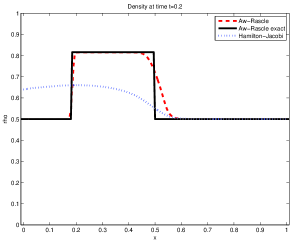
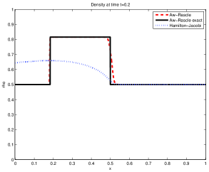
Example 1: In the first example the end of a traffic jam is considered. Thereby fast cars approach from the left a group of cars at rest on the right. The corresponding data is given by

$$\rho_{l}=0.5,\;u_{l}=1, \rho_{r}=0.5,\;u_{r}=0$$

and $x_{0}=0.5$. For the Rascle model the computations are performed in conservative form using the variables $(\rho,y=\rho(u-\mbox{ln}(1-\rho)))$ to obtain the correct shock speeds. The numerical results are shown in Figure 1. The exact solution of the Rascle model (solid line) is given by a shock-wave moving to the right followed by a stationary contact-discontinuity, see [3]. The numerical results for the Hamilton-Jacobi model (dotted line) show a faster braking of the approaching cars. This leads to a faster back-traveling wave and a less dense congested state. About the numerical aspects, the diffusion at the contact discontinuity is reduced by the finer grid, whereas the resolution of the shock in the Rascle model (dashed line) remains satisfactory.

Figure 1: Density $\rho$ at $t=0.2$ for the Riemann problem with $\rho_{l}=0.5,\;u_{l}=1,\;\rho_{r}=0.5,\;u_{r}=0$ and $x_{0}=0.5$.

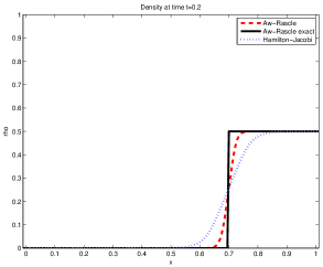
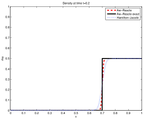
Example 2: Now the tail of a group of moving cars followed by an empty road is studied. The initial states are chosen as

$$\rho_{l}=0,\;u_{l}=1 \rho_{r}=0.5,\;u_{r}=1\ ,$$ and

with the discontinuity at $x_{0}=0.5$. As shown in Figure 2, the exact solution of the Rascle model (solid line) is given by a single contact-discontinuity moving at the speed of the leading cars. This behavior is captured well by the numerical scheme (dashed line) and holds also true for the Hamilton-Jacobi model. In both cases the cars are not influenced by the free space behind them and are thus following the constant state in front.

Figure 2: Density $\rho$ at $t=0.2$ for the Riemann problem with $\rho_{l}=0,\;u_{l}=1,\;\rho_{r}=0.5,\;u_{r}=1$ and $x_{0}=0.5$.

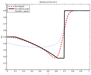
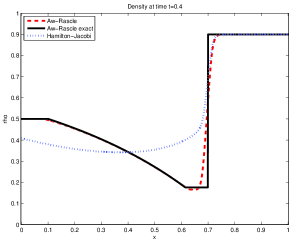
Example 3: Here we consider a group of faster vehicles escaping from slower ones in behind. Therefore we chose

$$\rho_{l}=0.5,\;u_{l}=0 \rho_{r}=0.9,\;u_{r}=0.5$$ and

on the left and right of $x_{0}=0.5$. In Figure 3 the corresponding solutions are plotted. The exact solution of the Rascle model (solid line) consists of a left going rarefaction wave and a contact-discontinuity moving to the right. As the drivers of the Hamilton Jacobi model (dotted line) tend to accelerate faster than those of the Rascle model (dashed line), the arising gap is less distinct. Thus a more homogeneous state is reached on the left. By increasing the number of grid points only the resolution of the contact discontinuity is improved.

Figure 3: Density $\rho$ at $t=0.4$ for the Riemann problem with $\rho_{l}=0.5,\;u_{l}=0,\;\rho_{r}=0.9,\;u_{r}=0.5$ and $x_{0}=0.5$.

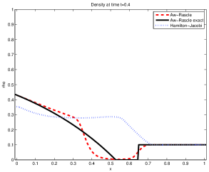
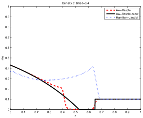
Example 4: Finally we consider an example similar to the above one, but now with faster cars on the right. The data is given as

$$\rho_{l}=0.5,\;u_{l}=0, \rho_{r}=0.1,\;u_{r}=1$$

and $x_{0}=0.25$. The exact solution of the Rascle model (solid line, Figure 4) is given by a rarefaction wave connected to a vacuum state, which is followed by a contact-discontinuity moving to the right. Here a difference to the numerical solution (dashed line) is observed. The applied scheme fails to properly capture the fake wave connecting the rarefaction wave to the vacuum state. The artificial jump can not be reduced by an increase of the computational accuracy. In the Hamilton Jacobi model (dotted line) no such vacuum state arises, since the drivers tend to accelerate faster.

Figure 4: Density $\rho$ at $t=0.5$ for the Riemann problem with $\rho_{l}=0.5,\;u_{l}=0,\;\rho_{r}=0.1,\;u_{r}=1$ and $x_{0}=0.25$.

In the above examples the wave fronts for the Hamilton-Jacobi model are smeared compared to the Aw-Rascle model as expected. In particular, Example 1 shows a stronger breaking for the Hamilton-Jacobi model and example 3 shows a faster acceleration of the vehicles keeping contact with the leading cars.

Remark 5.1

One also observes comparing the coarse and fine grid numerical solution, that the Hamilton-Jacobi equations are already well approximated by the coarse grid solution. Only example 4 shows a further steepening of the solution by refining the mesh. In general, the Rascle type conservation law is well approximated by the scheme except some smearing of the contact discontinuities. The only exception is the vacuum wave in example 4, where a non-physical jump is generated. Numerical difficulties at vacuum states are discussed e.g. in [22].

Remark 5.3

The numerical solution of the hyperbolic Aw-Rascle model is sensitive to the choice of variables. Example 1 (a solution with a shock) is computed using conservative variables $(\rho,y=\rho(u-\mbox{ln}(1-\rho))$ to ensure the correct intermediate state. Example 2,3,4 have been computed in $(\rho,\rho u)$ variables, since no shocks appear. Although this choice of variables improves the resolution of the contact discontinuity it remains rather diffusive. As mentioned above using the methods described in [21, 8] a sharp resolution of the contact discontinuities can be obtained. Nevertheless, we plotted in the above figures for comparison the solutions using the scheme described in Section 5.1.

Conclusions

• The paper contains the derivation of two classes of macroscopic models from kinetic equations. The type of equation one obtains does not depend on the fact whether an integro-differential equation or a Fokker-Planck type model is used, but rather on the fact which interaction rule is chosen.

• In certain cases a Hamilton-Jacobi term can be derived in the momentum equations instead of the classical Rascle term.

• Numerical investigation using a suitable second order method have been used to investigate the behavior of the solutions showing a smearing effect of the wave fronts for the Hamilton-Jacobi equations.

• Further investigations will include the derivation of suitable relaxation terms from kinetic models and multiphase traffic equations.

Acknowledgments

The present work has been supported by DFG KL 1105/16-1 and the DAAD PhD Program MIC.

References

• [1] A. Aw, Modèles hyperboliques de trafic automobile, PhD thesis, Nice, 2001.
• [2] A. Aw, A. Klar, T. Materne, and M. Rascle, Derivation of Continuum Traffic Flow Models from Microscopic Follow-the-Leader Models. SIAM J. Appl. Math. 63/1, 259-278, 2002
• [3] A. Aw and M. Rascle, Resurrection of second order models of traffic flow?, SIAM J. Appl. Math., 60 (2000), pp. 916–938.
• [4] S. Bryson, D. Levy, Central schemes for multidimensional Hamilton-Jacobi equations SIAM Sci. Comp. 25, 3, 767-791, 2003
• [5] Carrillo, J.A., D’Orsogna, M.R., Panferov, V.: Double milling in self-propelled swarms from kinetic theory. Kinetic and Related Models, 2 (2009), pp. 363-378.
• [6] F. Berthelin, P. Degond, M. Delitla, M. Rascle, A model for the formation and evolution of traffic jams Arch. Rat. Mech. Anal. 187, 185-220, 2008
• [7] F. Berthelin, P. Degond, V. Le Blanc, S. Moutari, J. Royer, M. Rascle, A Traffic-Flow Model with Constraints for the Modeling of Traffic Jams, Mathematical Models and Methods in Applied Sciences 18, 1269-1298, 2008
• [8] C. Chalons, P. Goatin, Transport-equilibrium schemes for computing contact discontinuities in traffic flow modelling, Commun. Math. Sci. Volume 5,3, 533-551, 2007
• [9] M. Günther, A. Klar, T. Materne, and R. Wegener, Multivalued fundamental diagrams and stop and go waves for continuum traffic flow equations. SIAM J. Appl. Math. 64/2, 468-483, 2003
• [10] J. Greenberg, Extension and amplification of the Aw-Rascle model, SIAM J. Appl. Math., 62 (2001), pp. 729–745.
• [11] D. Helbing, Gas-kinetic derivation of Navier-Stokes-like traffic equation, Physical Review E, 53 (1996), pp. 2366–2381.
• [12] M. Herty, R. Illner, On stop and go waves in dense traffic, Kinetic and Related Models (KRM),1, 2008, 437-452
• [13] R. Illner, A. Klar, and T. Materne, Vlasov-fokker-planck models for multilane traffic flow, Comm. Math. Sci., 1 (2003), pp. 1–12.
• [14] A. Klar and R. Wegener, Enskog-like kinetic models for vehicular traffic, J. Stat. Phys., 87 (1997), pp. 91–114.
• [15] A. Klar and R. Wegener, A hierachy of models for multilane vehicular traffic I: Modeling, SIAM J. Appl. Math., 59 (1998), pp. 983–1001.
• [16] A. Klar and R. Wegener, Kinetic derivation of macroscopic anticipation models for vehicular traffic, SIAM J. Appl. Math., 60 (2000), pp. 1749–1766.
• [17] P. Nelson, A kinetic model of vehicular traffic and its associated bimodal equilibrium solutions, Transport Theory and Statistical Physics, 24 (1995), pp. 383–408.
• [18] S. Paveri-Fontana, On Boltzmann like treatments for traffic flow, Transportation Research, 9 (1975), pp. 225–235.
• [19] H. Payne, FREFLO: A macroscopic simulation model of freeway traffic, Transportation Research Record, 722 (1979), pp. 68–75.
• [20] I. Prigogine and R. Herman, Kinetic Theory of Vehicular Traffic, American Elsevier Publishing Co., New York, 1971.
• [21] E.F. Toro, Riemann solvers and numerical methods for fluid dynamics, Springer, Berlin, Heidelberg, 2009.
• [22] E.F. Toro,Shock-Capturing Methods for Free-Surface Shallow Flows, John Wiley, 2001
• [23] G. Whitham, Linear and Nonlinear Waves, Wiley, New York, 1974.
• [24] W. Leutzbach, R. Wiedemann, Development and application of traffic simulation models at Karlsruhe Institut fuer Verkehrswesen, Traffic engineering and control, May, 20-278, 1986