Numerical bifurcation analysis of the pattern formation in a cell based auxin transport model

Abstract

Transport models of growth hormones can be used to reproduce the hormone accumulations that occur in plant organs. Mostly, these accumulation patterns are calculated using time step methods, even though only the resulting steady state patterns of the model are of interest. We examine the steady state solutions of the hormone transport model of Smith et al (2006) for a one-dimensional row of plant cells. We search for the steady state solutions as a function of three of the model parameters by using numerical continuation methods and bifurcation analysis. These methods are more adequate for solving steady state problems than time step methods. We discuss a trivial solution where the concentrations of hormones are equal in all cells and examine its stability region. We identify two generic bifurcation scenarios through which the trivial solution loses its stability. The trivial solution becomes either a steady state pattern with regular spaced peaks or a pattern where the concentration is periodic in time.

keywords:Bifurcation analysis, pattern formation, parameter dependence, auxin transport model, stability, periodic solution pattern PACS37N25 92C15 92C80

1 Introduction

1.1 Biological background

For centuries, the formation of well-defined patterns in plants, such as the orientation and shape of leaves, their venation patterns, the spatial distribution of hairs and stomata, the early embryonic development patterns and the branching patterns in both root systems and treetops, has intrigued many scientists. Experimental research has identified a number of molecular components that play a major role in several of these pattern formation processes. One of them is the plant hormone auxin, and more specifically the auxin molecule Indol-3-Acetic Acid (IAA). Experiments have shown that the active directional transport, which leads to accumulation spots of the auxin hormone, plays a central part in the pattern formation (Scarpella et al, 2006; Benková et al, 2003; Bilsborough et al, 2011).

Based on such experimental evidence, Reinhardt et al. developed a conceptual model that describes the auxin transport through the cells (Reinhardt et al, 2003). Smith and collaborators then constructed a computational simulation model (Smith et al, 2006) incorporating the experimental evidence that the transport of the auxin molecule IAA is driven by a pumping mechanism that is mediated by PIN1 proteins located at the cell membrane in addition to diffusion (Palme and Gälweiler, 1999). Therefore, Smith and collaborators modeled the transport of the IAA hormone through the cells by describing the simultaneous evolution of the PIN1 protein and the IAA hormone concentrations over time. Also other computational models were developed based on these molecular mechanisms identified by Reinhardt et al.. For instance Jönsson et al. proposed a phyllotaxis model based on the polarized auxin transport (Jönsson et al, 2006). They analyzed a simplified version of their model that assumes an equal and constant PIN1 concentration in every cell and membrane. In their simulations they used a linear row of uniform cells with periodic boundary conditions. The results show that the spacing and the number of peaks in this simplified model depends on the different parameters. Jönsson and collaborators also performed a stability analysis and found an analytical expression for the eigenvalues, belonging to a solution pattern with equal auxin concentrations. The eigenvalues are all real and a function of the model parameters of the model. They also identified the parameter threshold where the largest eigenvalue becomes unstable. Beyond this threshold, all stable solutions will contain auxin peaks.

This paper expands the study of the steady states in the transport of hormones. We limit ourselves to the study of the auxin distribution in a linear row of uniform cells that represents, for example, a cross section through a young leaf. We perform a thorough mathematical exploration of the behavior of the models and how their equations are solved starting from the basic coupled model of Smith et al (2006). In contrast to the analysis of Jönsson et al. on a row of cells with fixed concentration of PIN1, we will use a coupled model where the PIN1 concentration is allowed to change from cell to cell. The analysis gives new insights into the spacing of auxin accumulations that form the basis of vascular development (Scarpella et al, 2006).

The patterns that emerge in a dynamical system are often studied mathematically through a bifurcation analysis. It relates the stability of the patterns to the parameters that occur in the systems description. The transitions where the patterns lose their stability are bifurcation points. For an overview of the bifurcation analysis of patterns we refer to the book (Hoyle, 2006).

The main contribution of the paper is a systematic numerical bifurcation analysis for the coupled model of Smith et al (2006) describing the transport of auxin. The analysis identifies two generic bifurcation scenarios that reappear for various choices of the parameters of the problem. Through the bifurcation diagrams we identify the genesis of the patterns that were observed by Smith and collaborators. Furthermore, we have found a limited parameter range that allows periodic solutions in the system. In these solutions, the concentration of auxin of each cell varies periodically over time. To the knowledge of the authors these results have not appeared in the literature.

We present our work as follows. In section 1.2 the basic cell polarization and auxin transport model of Smith et al (2006), where PIN1 is allowed to change, is reconstructed. We also introduce a slightly generalized version of the active transport equation of this model. In the next section, a specific model that will be used in the simulations is defined. In Smith et al (2006) the domain roughly correlates to a ring of cells around an axial plant organ. In subsequent situations we consider a linear row of cells running from the margin to the midvein of the leaf and we consider zero fluxes at the boundary of the leaf. We will describe this by using homogeneous Neumann boundary conditions instead of periodic boundary conditions which is explained in section 2.1. Also in this section we look at the different parameter values. Similar to Smith et al., we use time integration to solve the coupled equations of Smith et al. in section 2.2. Since we are only interested in the steady state solutions, we define in section 2.3, the corresponding steady state systems of the slightly different equations. For these steady state models, we define in section 3 a trivial solution and its stability properties. The stability is dependent on the model parameters and we examine for which parameter regions the trivial solution is stable. Section 4 contains the techniques that will be used to solve the models. In particular, we will discuss bifurcation analysis (4.1) and continuation methods (4.2). Bifurcation analysis reveals the relation between the stability of a solution and the model parameters and continuation methods calculates approximate solutions in function of a model parameter. In section 5 we show the results of our simulations. In section 6 we conclude and give an outlook.

1.2 Description of the mathematical model

Before constructing a compartmental model that describes the concentration of growth hormones per cell and its transport through a plant organ such as for example a leaf, its geometry must be specified.

1.2.1 Geometry of the cells

The domain in this work is a regular one dimensional row of cells, as in figure 1. Each cell is labeled and the set of cells is denoted with $V$. Therefore, for every cell in $V$, we can define the neighboring cells, a subset of $V$. For example, $\mathcal{N}_{i}=\left\{i-1,i+1\right\}$ is the set of neighboring cells of cell $i$. Further every cell consists of a number of cell walls. The length of a cell wall between cell $i$ and cell $j$ is denoted with $l_{ij}=l_{ji}$.

The one dimensional domain in figure 1 represents the 1D geometry of a group of cells in a part of a plant organ at a certain moment in time. In advanced models this geometry changes over time because cell walls grow and cells divide (Smith et al, 2006), but in this paper we look at the basic, coupled cell polarization and auxin transport model of Smith et al. and the geometry is assumed to be static. As a consequence the row of cells is fixed. The length of the cell wall is taken to be the length unit. As a result the volume of a cell also is the unit volume.

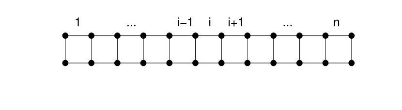
Figure 1: The one-dimensional domain, a row of regular square cells from $1$ to $n$.

1.2.2 Transport of growth hormones

For this geometry it is now possible to formulate a model for the transport of the growth hormones through the cells. We will write down with a concise mathematical notation the coupled equations of Smith et al (2006) applied to a section across a leaf with the geometry specified above. Subsequently we introduce a slight generalization of the active transport term in the equation.

In every cell $i$ two substances play an important role in the growth process:

• The concentration of proteins PIN$1$ in cell $i$, which is time dependent, is denoted as $\left[\textrm{PIN}1\right]_{i}\left(t\right)\in\mathbb{R}^{+}$ and is measured in micromol, i.e 10^-6mol, over the unit volume. We use the dimensionless variable $p_{i}\left(t\right)=\left[\textrm{PIN}1\right]_{i}\left(t\right)/\mu$M.

• The concentration of the hormone IAA in cell $i$, also known as auxin, is also time dependent and is denoted as $\left[\textrm{IAA}\right]_{i}\left(t\right)\in\mathbb{R}^{+}$. Again in units of $\mu$M. We use the dimensionless variable $\left[\textrm{IAA}\right]_{i}\left(t\right)/\mu$M, which is denoted as $a_{i}\left(t\right)$.

The model describes the evolution of these dimensionless concentrations in each cell. This evolution depends in a non-linear way on the concentrations of the neighboring cells. The value of $p_{i}\left(t\right)$ is determined by the production and decay of PIN$1$. Its time evolution for each cell $i\in V$ is modeled by

$$\dfrac{dp_{i}\left(t\right)}{dt}=\dfrac{\rho_{{}_{\textnormal{{\tiny PIN}}_{0}}}+\rho_{{}_{\textnormal{{\tiny PIN}}}}a_{i}\left(t\right)}{1+\kappa_{{}_{\textnormal{{\tiny PIN}}}}p_{i}\left(t\right)}-\mu_{{}_{\textnormal{{\tiny PIN}}}}p_{i}\left(t\right),$$ (1)

where $\rho_{{{}_{\textnormal{{\tiny PIN}}}}_{0}}\in\mathbb{R}^{+}$ is the base production of PIN1 proteins and $\rho_{{}_{\textnormal{{\tiny PIN}}}}\in\mathbb{R}^{+}$ is a coefficient capturing the up-regulation of PIN1 production by auxin, both measured per second, $\kappa_{{}_{\textnormal{{\tiny PIN}}}}\in\mathbb{R}^{+}$ is the saturation coefficient of the PIN1 production, which is dimensionless, and $\mu_{{}_{\textnormal{{\tiny PIN}}}}\in\mathbb{R}^{+}$ is the PIN1 decay constant, which has units of $1$/s. This means that the evolution of $p_{i}\left(t\right)$ in time depends strictly on the concentration in the cell itself.

The concentration of IAA in a cell depends not only on the production and the decay of auxin in the cell. Change of $a_{i}\left(t\right)$ is also determined by diffusion (passive transport) and active transport of auxin between the cells. The change over time of the concentration of IAA is modeled by the equation

$$\dfrac{da_{i}\left(t\right)}{dt} = \dfrac{\rho_{{}_{\textnormal{{\tiny IAA}}}}}{1+\kappa_{{}_{\textnormal{{\tiny IAA}}}}a_{i}\left(t\right)}-\mu_{{}_{\textnormal{{\tiny IAA}}}}a_{i}\left(t\right)-\sum_{j\in\mathcal{N}_{i}}\textnormal{D}\left(a_{i}\left(t\right)-a_{j}\left(t\right)\right)$$

$$\left.\right.\hskip 14.22636pt+\sum_{j\in\mathcal{N}_{i}}\left(\text{ActiveTransport}_{j\rightarrow i}-\text{ActiveTransport}_{i\rightarrow j}\right),$$

where $\rho_{{}_{\textnormal{{\tiny IAA}}}}\in\mathbb{R}^{+}$ is the IAA production coefficient which is measured per second, $\kappa_{{}_{\textnormal{{\tiny IAA}}}}\in\mathbb{R}^{+}$ is the dimensionless coefficient which controls the saturation of IAA production, $\mu_{{}_{\textnormal{{\tiny IAA}}}}\in\mathbb{R}^{+}$ is the IAA decay constant and $D\in\mathbb{R}^{+}$ is the IAA diffusion coefficient, both measured per second. The active transport depends on the presence of PIN1 denoted by $p_{i}$ and is modeled by the formula

$$\text{ActiveTransport}_{i\rightarrow j}=\textnormal{T}\left(\dfrac{p_{i}\left(t\right)l_{ij}\textnormal{b}^{a_{j}\left(t\right)}}{\sum_{k\in\mathcal{N}_{i}}{l_{ik}\textnormal{b}^{a_{k}\left(t\right)}}}\right)\dfrac{a_{i}\left(t\right)^{2}}{1+\kappa_{{}_{\textnormal{{\tiny T}}}}a_{j}\left(t\right)^{2}},$$ (3)

where $T\in\mathbb{R}^{+}$ is a polar IAA transport coefficient expressed per second, $b\in\mathbb{R}^{+}$ is the exponentiation base which controls the extent to which the PIN1 protein distribution is affected by the neighboring cells and $\kappa_{{}_{T}}\in\mathbb{R}^{+}$ is an IAA transport saturation coefficient. These parameters are dimensionless. From equation (1.2.2) we know that the evolution of $a_{i}(t)$ depends only on itself, the first and the second nearest neighbors of cell $i$. Since we can specify the neighbors for every cell, the second nearest neighbors can be easily determined. For example the second neighbors of cell $i$ are all elements in $\bigcup_{j\in\mathcal{N}_{i}}\mathcal{N}_{j}$. Remark that because the length of each cell wall is taken to be the length unit, it cancels from the equation.

Equations (1), (1.2.2) and (3) describe the basic coupled model of Smith et al. that has been used to study the transport of hormones in the Arabidopsis shoot apex. It differs mainly from other transport models by the active transport term. Smith et al. uses a quadratic dependence to describe the flux on the auxin concentrations instead of a linear dependence. Further they introduce an exponential dependence of the localization of PIN1 on the concentration of IAA. Therefor we will also consider two other models. One where the active transport is modeled with a linear dependence to describe the flux on the auxin concentration

$$\text{ActiveTransport}_{i\rightarrow j}=\textnormal{T}\left(\dfrac{p_{i}\left(t\right)\textnormal{b}^{a_{j}\left(t\right)}}{\sum_{k\in\mathcal{N}_{i}}{\textnormal{b}^{a_{k}\left(t\right)}}}\right)\dfrac{a_{i}\left(t\right)}{1+\kappa_{{}_{\textnormal{{\tiny T}}}}a_{j}\left(t\right)},$$ (4)

and one model without the exponential dependence of the localization of PIN1 on the concentration of IAA

$$\text{ActiveTransport}_{i\rightarrow j}=\textnormal{T}\left(\dfrac{p_{i}\left(t\right)a_{j}\left(t\right)}{\sum_{k\in\mathcal{N}_{i}}{a_{k}\left(t\right)}}\right)\dfrac{a_{i}\left(t\right)^{2}}{1+\kappa_{{}_{\textnormal{{\tiny T}}}}a_{j}\left(t\right)^{2}}.$$ (5)

The three different equations that model the active transport (equations (3), (4) and (5)) can be combined in one generalized equation

$$\text{ActiveTransport}^{\omega,\tau}_{i\rightarrow j}=\textnormal{T}\left(\dfrac{p_{i}\left(t\right)\left(\omega\textnormal{b}^{a_{j}\left(t\right)}+\left(1-\omega\right)a_{j}\left(t\right)\right)}{\sum_{k\in\mathcal{N}_{i}}{\left(\omega\textnormal{b}^{a_{k}\left(t\right)}+\left(1-\omega\right)a^{k}\left(t\right)\right)}}\right)\dfrac{a_{i}\left(t\right)^{\tau}}{1+\kappa_{{}_{\textnormal{{\tiny T}}}}a_{j}\left(t\right)^{\tau}},$$ (6)

For $\omega=1$ and $\tau=2$, (1), (1.2.2) and (6) describe the equations of Smith et al (2006).

In Smith et al (2006) a row of 50 equal sized cells with periodic boundary conditions was investigated. The results of the time evolution, starting from an initially flat solution with a small amount of noise to break symmetry, showed the emergence of a pattern in the IAA concentrations (figure 2). Some cells have a very high concentration of auxin. It was found that the peaks in a pattern are equally spaced and become more prominent for an increasing IAA transport coefficient T.

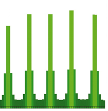
Figure 2: Simulation results of Smith et al (2006) for a one dimensional row of $50$ cells with periodic boundary conditions. The shades of green show a difference in the IAA concentration. (figure reproduced from Smith et al (2006)).

2 The simulation problem

2.1 Domain, boundary conditions and parameters

In this paper we analyze the solutions of equations (1) and (1.2.2), for a one dimensional file of equal sized square cells. We assume that this file of cells represents a part of a leaf from the left margin to the midvein. This assumption is necessary in order to specify the boundary condition. Other parts of plant organs can give rise to other boundary conditions which will result in a small change in the model.

To provide the boundary conditions, two ghost cells are required at each end of the domain, since the model relates each cell with two cells at the left and the right (figure 3).

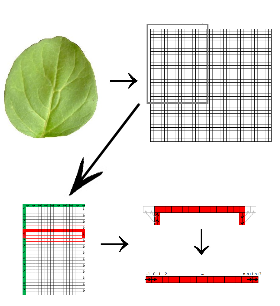
Figure 3: The one-dimensional model can be seen as a row of cells cut out of a leaf with equal sized square cells. In the first step we represent the leaf as a two dimensional squared grid of equal sized square cells. The second arrow indicates that we only consider the part from the left margin till the midvein. Here in each cell at the boundary, the direction of the auxin fluxes is indicated. In the third step a horizontal row of inner cells with, at each side two boundary cells is cut out of the domain. In the last step this domain is enrolled so it forms a one dimensional file of equal sized square cells. The two boundary cells at each side of the domain are the ghost cells.

The $n$ interior cells are labeled $1$ to $n$. The ghost cells are cells $-1$ and $0$ at the left of the domain and cells $n+1$ and $n+2$ at the right. The concentration of the IAA hormone in the two ghost cells on each side are chosen to describe the influx at the boundary of the leaf and the efflux at the vein. The IAA concentration then changes linearly at the boundaries as if Neumann boundary conditions are applied. We assume zero flux boundary conditions. This means that the boundary conditions become

$$\begin{cases}a_{-1}\left(t\right)=a_{1}\left(t\right)\quad\text{and}\quad a_{0}\left(t\right)=a_{1}\left(t\right),\\ a_{n+1}\left(t\right)=a_{n}\left(t\right)\quad\text{and}\quad a_{n+2}\left(t\right)=a_{n}\left(t\right).\end{cases}$$ (7)

The value of $p_{0}\left(t\right)$ and $p_{n+1}\left(t\right)$ in the ghost cells is determined by equation (1) that couples it to the value of $a_{i}\left(t\right)$ in the ghost cell. Note that $p_{-1}\left(t\right)$ and $p_{n+2}\left(t\right)$ do not appear in the problem since equation (3) does not require it. Together with an initial condition, the problem is transformed in an initial value problem that we can solve numerically with a time step method. Remark that these homogeneous Neumann boundary conditions are different from periodic boundary conditions. The concentrations in the cells on the left side of the domain can indeed be different from the concentrations in the cells on the right side of the domain.

Equations (1), (1.2.2) and (3) contain $11$ parameters. A short description can be found in table 1 and further details can be found in Smith et al (2006). The values of these parameters must be real and positive. For the simulations in this paper we used three different parameter sets, M1, M2 and M3. Parameter set M2 corresponds with the values used by Smith et al (2006). Parameter set M1 and M3 contain the same values for the parameters as set M2 except for the IAA production coefficient. The value of this parameter is higher in parameter set M1 and lower in set M3.

Table 1: Values of the parameters of equations (1)–(3) used in the simulations. The parameter values of M2 are found in Smith et al (2006).

Symbol	Description	Value
		M1	M2	M3
b	Base for exponential PIN allocation	$3.000$	$3.000$	$3.000$
$\kappa_{{}_{\textnormal{{\tiny PIN}}}}$	PIN saturation coefficient	$1.000$	$1.000$	$1.000$
$\kappa_{{}_{\textnormal{{\tiny T}}}}$	Transport saturation coefficient	$1.000$	$1.000$	$1.000$
$\kappa_{{}_{\textnormal{{\tiny IAA}}}}$	IAA saturation coefficient	$1.000$	$1.000$	$1.000$
$\rho_{{}_{\textnormal{{\tiny PIN}}_{0}}}$	Base production of PIN	$0.000$	$0.000$	$0.000$
$\rho_{{}_{\textnormal{{\tiny PIN}}}}$	PIN production coefficient	$1.000$	$1.000$	$1.000$
$\mu_{{}_{\textnormal{{\tiny PIN}}}}$	PIN decay coefficient	$0.100$	$0.100$	$0.100$
$\mu_{{}_{\textnormal{{\tiny IAA}}}}$	IAA decay coefficient	$0.100$	$0.100$	$0.100$
$\rho_{{}_{\textnormal{{\tiny IAA}}}}$	IAA production coefficient	$1.500$	$0.750$	$0.500$
D	IAA diffusion coefficient	$1.000$	$1.000$	$1.000$
T	IAA transport coefficient	$3.500$	$3.500$	$3.500$

2.2 Time integration

Similar to Smith et al (2006), we can solve the initial value problem of Smith and collaborators with numerical integration. Analysis of the eigenvalues of the Jacobian shows that they are mostly located along the negative real axis with some small complex conjugate pairs of outliers at the left of the imaginary axis. This suggests that the fourth order Runge-Kutta method (Hairer et al, 2009) with time step $\Delta t=0.01$ results in a stable method to integrate the equations.

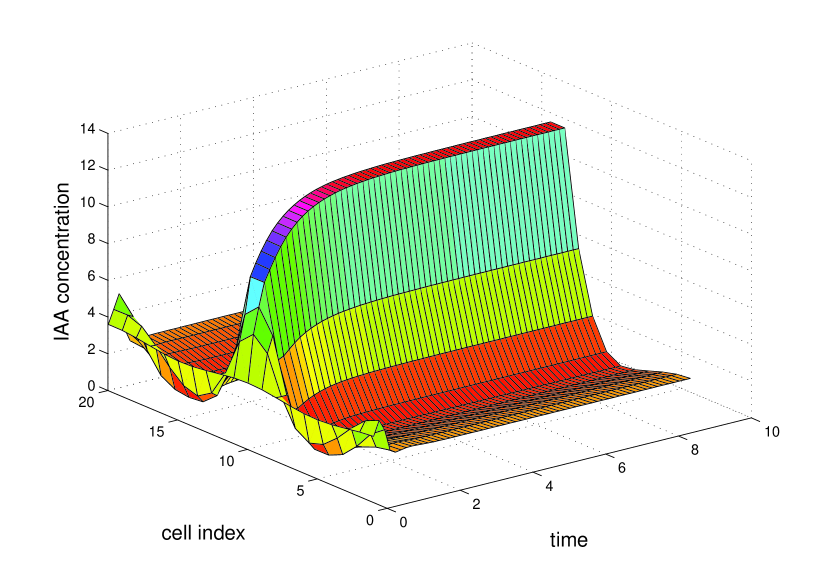
Figure 4: The time evolution of the solution of equations (1), (1.2.2) and (3) for a row of 20 cells with zero Neumann boundary condition and parameter set M1. The initial condition is given by equation (8) and we used RK4 for numerical integration.

In figure 4 the time evolution is shown from $t=0$ to $t=10$. The domain contains $20$ cells plus $4$ ghost cells where we assume zero Neumann boundary conditions. The parameter values of set M1 are used and the initial value for the concentration is

$$p_{i}(t=0)=5.4\quad\text{and}\quad a_{i}(t=0)=3.4,$$ (8)

where a small perturbation $0.2\sin\left(\left(5\left(i+2\right)\pi\right)/24\right)$ for $i=1,\ldots,20$ was added to it to break symmetry. Any other initial state nearby will lead to the same long term solution.
Figure 4 shows the development of a pattern in the concentration of auxin. After a certain time the pattern arrives in a stable steady state. For the row of $20$ cells a single peak with a high IAA concentration is formed.

2.3 Steady state problem

Rather than evolving the system in time, we can calculate the steady state solutions directly. We rewrite equations (1), (1.2.2) and (3) in order to obtain the steady state equations for this specific geometry and boundary conditions. The steady state problem becomes:

$$\begin{cases}0&=\dfrac{\rho_{{}_{\textnormal{{\tiny PIN}}_{0}}}+\rho_{{}_{\textnormal{{\tiny PIN}}}}a_{i}}{1+\kappa_{{}_{\textnormal{{\tiny PIN}}}}p_{i}}-\mu_{{}_{\textnormal{{\tiny PIN}}}}p_{i}\quad\text{with}\quad i=0,1,\ldots,n,n+1\\ 0&=\dfrac{\rho_{{}_{\textnormal{{\tiny IAA}}}}}{{1+\kappa_{{}_{\textnormal{{\tiny IAA}}}}}a_{i}}-\mu_{{}_{\textnormal{{\tiny IAA}}}}a_{i}-{\textnormal{D}\left(a_{i}-a_{i-1}\right)}-{\textnormal{D}\left(a_{i}-a_{i+1}\right)}\\ &+\textnormal{T}\left(\dfrac{p_{i-1}\textnormal{b}^{a_{i}}}{\textnormal{b}^{a_{i-2}}+\textnormal{b}^{a_{i}}}\right)\dfrac{a_{i-1}^{2}}{1+\kappa_{{}_{T}}a_{i}^{2}}-\textnormal{T}\left(\dfrac{p_{i}\textnormal{b}^{a_{i-1}}}{\textnormal{b}^{a_{i-1}}+\textnormal{b}^{a_{i+1}}}\right)\dfrac{a_{i}^{2}}{1+\kappa_{{}_{T}}a_{i-1}^{2}}\\ &+\textnormal{T}\left(\dfrac{p_{i+1}\textnormal{b}^{a_{i}}}{\textnormal{b}^{a_{i}}+\textnormal{b}^{a_{i+2}}}\right)\dfrac{a_{i+1}^{2}}{1+\kappa_{{}_{T}}a_{i}^{2}}-\textnormal{T}\left(\dfrac{p_{i}\textnormal{b}^{a_{i+1}}}{\textnormal{b}^{a_{i-1}}+\textnormal{b}^{a_{i+1}}}\right)\dfrac{a_{i}^{2}}{1+\kappa_{{}_{T}}a_{i+1}^{2}}\\ &\hskip 199.16928pt\textrm{with }\quad i=1,\ldots,n\\ \\ &a_{-1}=a_{1}\quad\text{and}\quad a_{0}=a_{1}\\ &a_{n+1}=a_{n}\quad\text{and}\quad a_{n+2}=a_{n},\end{cases}$$ (9)

where the indices $0$ and $n+1$ in the first equation express the coupling of $p_{i}$ to $a_{i}$ in the first ghost cells. This system can be written as the system of equations

$$F\left(\mathbf{U},\boldsymbol{\lambda}\right)=\mathbf{0},$$ (10)

where $F:\mathbb{R}^{2n+m}\longrightarrow\mathbb{R}^{2n}:\left(\mathbf{U},\boldsymbol{\lambda}\right)\mapsto F\left(\mathbf{U},\boldsymbol{\lambda}\right)$ with $n$ the number of cells and $m$ the number of parameters. $\mathbf{U}$ is a $2n$ dimensional solution vector of the problem that contains both the $p$ and $a$ steady state variables and $\boldsymbol{\lambda}\in\mathbb{R}^{m}$ denotes the set of parameters.

For the equations (1) and (1.2.2) with active transport equations (4), (5) or (6) the steady state problem can be obtained in the same way.

3 The trivial solution

In this section we search for a trivial solution of system (9), a solution that can be calculated analytically and that will be used as a starting point for the numerical continuation in section 5.

If we assume that the solution is homogeneous then the values of $p$ and $a$ are the same for all cells so that

$$p_{i}=p_{j}\quad\text{and}\quad a_{i}=a_{j}\qquad\forall i,j=-1,\ldots,n+2.$$ (11)

The system (9) now reduces to

$$\begin{cases}0=\dfrac{\rho_{{}_{\textnormal{{\tiny PIN}}_{0}}}+\rho_{{}_{\textnormal{{\tiny PIN}}}}a_{i}}{1+\kappa_{{}_{\textnormal{{\tiny PIN}}}}p_{i}}-\mu_{{}_{\textnormal{{\tiny PIN}}}}p_{i}\quad\text{ for }i=0,\ldots,n+1\\ 0=\dfrac{\rho_{{}_{\textnormal{{\tiny IAA}}}}}{{1+\kappa_{{}_{\textnormal{{\tiny IAA}}}}}a_{i}}-\mu_{{}_{\textnormal{{\tiny IAA}}}}a_{i}\quad\text{ for }i=1,\ldots,n,\end{cases}$$ (12)

and

$$a_{-1}=a_{0}=a_{1}\quad\text{and}\quad a_{n+1}=a_{n+2}=a_{n}.$$ (13)

Because $p_{i}$ and $a_{i}$ are real positive numbers, we find a unique solution that is given by

$$\begin{cases}p_{i}=\dfrac{-1+\sqrt{1+4\kappa_{{}_{\textnormal{{\tiny PIN}}}}\left(\rho_{{}_{\textnormal{{\tiny PIN}}_{0}}}+\rho_{{}_{\textnormal{{\tiny PIN}}}}a_{i}\right)/\mu_{{}_{\textnormal{{\tiny PIN}}}}}}{2\kappa_{{}_{\textnormal{{\tiny PIN}}}}},\\ a_{i}=\dfrac{-1+\sqrt{1+4\kappa_{{}_{\textnormal{{\tiny IAA}}}}\rho_{{}_{\textnormal{{\tiny IAA}}}}/\mu_{{}_{\textnormal{{\tiny IAA}}}}}}{2\kappa_{{}_{\textnormal{{\tiny IAA}}}}},\end{cases}$$ (14)

with $i=-1,\ldots,n+2$. This is the trivial solution of the system. Note that the same trivial solution is obtained for the models with active transport equation (4), (5) or (6) . From equation (12) we know that for a certain parameter set, there is only one trivial homogeneous solution. By formula (14) it is easy to calculate this trivial solution for different parameter values. Figure 5 shows the concentration of IAA in one cell (cell number 6) versus the parameter $\rho_{{}_{\textnormal{{\tiny IAA}}}}$. Because the solution is homogeneous, the trivial solution curve would be the same for every cell and is independent of the number of cells. Figure 5 denotes also the trivial solution for parameter set M1, M2 and M3 with a square.

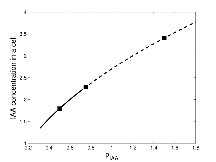
Figure 5: The concentration of IAA in the trivial solution as a function of the IAA production coefficient $\rho_{\textnormal{{\tiny IAA}}}$. Each cell has the same concentration. However, for large $\rho_{\textnormal{{\tiny IAA}}}$ this solution becomes unstable. Stability is calculated for equation (9) and a row of 20 cells. The other parameters are taken from table 1.

3.1 Stability of the trivial solution

The value of the IAA concentration in the trivial solution is independent of the IAA diffusion coefficient D and the IAA transport coefficient T. Furthermore, it does not depend on the type of model for the active transport. Any choice of $\omega$ or $\tau$ yields to the same trivial solution. However, the stability depends in a sensitive way on the diffusion and transport coefficients and on the model of the active transport. Although expression (14) for the trivial solution is readily obtained, it is not easy to determine the stability of this solution. The Jacobian matrix of the coupled system (9) is not trivial. It has a sparse blocked structure where the first top-left block is diagonal and contains the linearization of Eq. (1). The top-right block is also diagonal and has the derivative of Eq. (1) to $a_{i}$. The bottom-left block is tridiagonal since the active transport in cell $i$ depends on $p_{i-1}$, $p_{i}$ and $p_{i+1}$. Finally, the bottom right block has five diagonals because the active transport depends on the neighbors and the neighbors of the neighbors. Because of the complicated structure the eigenvalues are non-trivial and we have found that for the coupled problem they are not necessarily real valued in contrast to the results of the uncoupled problem, see for example (Jönsson et al, 2006).

The stability can, however, easily be calculated by numerical means and in our simulations we approximate the Jacobian with central finite differences. The $j$-th column of $J(\mathbf{U},\boldsymbol{\lambda})$ is $J(\mathbf{U},\boldsymbol{\lambda})\mathbf{e}_{j}$ where $\mathbf{e}_{j}$ is the unit vector with the $j$-th component equal to 1 and the other components equal to 0. The column is then approximated as

$$J(\mathbf{U},\boldsymbol{\lambda})\mathbf{e}_{j}=\frac{F(\mathbf{U}+\epsilon\mathbf{e}_{j},\boldsymbol{\lambda})-F(\mathbf{U}-\epsilon\mathbf{e}_{j},\boldsymbol{\lambda})}{2\epsilon},$$ (15)

where $\epsilon$ is taken of the order of 10^-7. Once an approximation to the Jacobian is obtained, its eigenvalues can be calculated. This numerical approach can also be used to study the stability of other solutions.

The stability of the trivial solution of equation (9) for a row of $20$ cells is shown in figure 5. For smaller values of $\rho_{{}_{\textnormal{{\tiny IAA}}}}$ the eigenvalues of the trivial solutions lie in the left half-plane of the complex plane. Therefor these stable solutions are drawn with a full line in figure 5. For larger values of $\rho_{{}_{\textnormal{{\tiny IAA}}}}$, at least one eigenvalue lies in the right half plane and so the trivial solution is unstable. This is indicated with a dotted line.

Also for other parameter values we can calculate the stability of the trivial solution. In each plot on figure 6 two parameter values are varied. The other parameter values are taken as in parameter set M2. The first row of figures corresponds with the stability region for equation (9) ( i.e. the basic coupled model of Smith et al (2006)) and the second row of figures represents the stability regions for the steady state problem with a modified active transport equation (4). These plots show where the trivial solution is stable (marked in gray) for a row of $20$ cells.

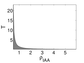
(a)

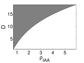
(b)

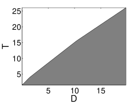
(c)

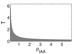
(d)

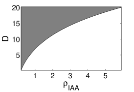
(e)

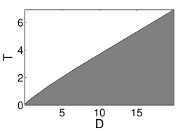
(f)

Figure 6: Stable (marked in gray) and unstable region of the trivial solution for a row of 20 cells and different choices of the parameters $\rho_{\textnormal{{\tiny IAA}}}$ (IAA production coefficient), D (IAA diffusion coefficient) and T (IAA transport coefficient). Other parameters are taken from parameter set M2. The first row of figures displays the stability regions for the model with active transport equation (3), the second row for the model with active transport equation (4).

For example, figure 6a shows that very small values of $\rho_{{}_{\textnormal{{\tiny IAA}}}}$ give a stable trivial solution for almost every value of T in the original model. All other values of $\rho_{{}_{\textnormal{{\tiny IAA}}}}$ give an unstable trivial solution if T is not too small. Further we find that when the active transport is modeled with a linear dependence on the auxin concentration, the shape of the stability region of the trivial solution remains approximately the same but it is much smaller than with a quadratic dependency (compare for example figure 6a and figure 6d). For both models we find that increasing the number of cells, leads to approximately the same shape of the stable region of the trivial solution – it only gets slightly smaller. Applying the model without the exponential dependence of the localization of PIN1 on the concentration of IAA results in a stable trivial solution for the entire tested range of parameters.

4 Methods

4.1 Bifurcation analysis

The study of the relation between the stability of a solution and the parameters of the corresponding dynamical system is known as bifurcation analysis (Seydel, 1994). Such an analysis identifies the stable and unstable solutions and the bifurcation points that mark the transitions between them. This is biologically relevant since it will allow us to predict the patterns that emerge in the time evolution as the parameters of the model are changed. A bifurcation point is a solution $\left(\textbf{U}_{i},\boldsymbol{\lambda}_{i}\right)$ of system (10) where the number of solutions changes when $\boldsymbol{\lambda}$ passes $\boldsymbol{\lambda}_{i}$. In this article there are several types of bifurcation points such branch points, limit points and Hopf bifurcation points that will play a role. A branch point is a bifurcation point where two or more branches with distinct tangents intersect. A limit point, also called a turning point, is a point where, locally, no solutions exist on one side of the limit point and two solutions on the other side. A Hopf bifurcation is a transition where a periodic orbit appears and branch points and limit points are both bifurcation points among steady state solutions. For complete review of their properties wer refer to (Seydel, 1994). The analysis usually leads to a bifurcation diagram that highlights the connections between stable and unstable branches as the parameters change. It is useful to track all these solution branches that emerge, split or end in a bifurcation point. This can be done with the help of numerical continuation methods.

4.2 Continuation methods

The system of equations (10) is a smooth map and we know that $\mathbf{0}\in\text{Range}\left(F\right)$. Following the implicit function theorem we know that for a regular point $\mathbf{x}_{0}=\left(\mathbf{U}_{0},\boldsymbol{\lambda}_{0}\right)\in\mathbb{R}^{2n+m}$ of $F$ that satisfies $F\left(\mathbf{x}_{0}\right)=\mathbf{0}$, the solution set $F^{-1}\left(\mathbf{0}\right)$ can be locally parametrized about $\mathbf{x}_{0}$ with respect to some parameter $s$. This means that the system of equations $F\left(\mathbf{U},\boldsymbol{\lambda}(s)\right)=\mathbf{0}$ defines an implicit curve $\mathbf{U}(\boldsymbol{\lambda}(s))$ where $\boldsymbol{\lambda}(s):\mathbb{R}\rightarrow\mathbb{R}^{m}$ is any parametric curve in the $\mathbb{R}^{m}$ (Allgower and Georg, 1994). The idea of continuation methods is to find a curve $c$ of approximate solutions U of the system in function of the parameter $\boldsymbol{\lambda}(s)$. To construct such a curve of subsequent solution points $\mathbf{x}_{i}=\left(\mathbf{U}_{i},\boldsymbol{\lambda}_{i}\right)=\left(\mathbf{U}_{i},\boldsymbol{\lambda}(s_{i})\right)$, continuation methods use a starting point $\mathbf{x}_{0}=\left(\mathbf{U}_{0},\boldsymbol{\lambda}_{0}\right)$, a solution of system (10), along with an initial continuation direction (Krauskopf et al, 2007). This starting point is typically a trivial solution. An important family of the continuation methods are the predictor-corrector methods such as pseudo-arc-length continuation. The idea of the algorithm is to first predict a new solution point. In the corrector step, this predicted point is the start value for an iterative method that will approximate the solution to a given tolerance. For the pseudo-arc-length, the predictor step uses the tangent vector to the curve at a solution point and a given step size to predict a guess for the next solution point on the curve. The corrector step improves the guess with Newton iterations.

Numerical continuation is available in AUTO (Doedel et al, 1997), LOCA part of Trilinos (Salinger et al, 2005), PyDS (Clewley et al, 2007) and others. These libraries can often also identify the bifurcations that occur along the continued curve and some of them, such as AUTO can automatically switch between branches at bifurcation points.

5 Results

This section presents several examples that highlight specific properties of the dynamics of the model. In the first three examples we give, for a file of $20$ cells, the numerical bifurcation analysis of equation (9) with respectively parameter sets M1, M2 and M3. In the fourth example, we enlarge the system and study now a file of $100$ cells with parameter set M1 instead of $20$ cells. In the last two examples we investigate the model with a generalized equation for the active transport. In example 5, we look at the influence of the parameter $\tau$ on the bifurcation scheme found in example $1$. Finally in example $6$ we investigate the influence of the parameter $\omega$ on the stability.

In examples $1$ to $5$ the IAA transport coefficient T is the continuation parameter. We have chosen T as the continuation parameter similar to the one-dimensional simulations of Smith et al (2006). Also Jönsson et al (2006) investigated the influence of the IAA transport coefficient T in their simple model by changing the ratio D/TP, with P the fixed value for PIN1. In example 6 we use $\omega$ as continuation parameter.

Each time we choose to display a bifurcation diagram that depicts the IAA concentration in cell number $6$ versus the continuation parameter. Alternative choices for the measure on the y-axis (e.g. a different cell) would be equally valid.

We will find that the trivial solution loses its stability through either a branch point or a Hopf bifurcation. The results also show the small effect of the quadratic dependence in comparison with the linear dependence to describe the flux on the auxin concentration.

Example 1.

This example illustrates the first generic scenario that is encountered when the trivial solution loses its stability. The results of the bifurcation analysis for equation (9) and parameter set M1 are shown in figure 7.

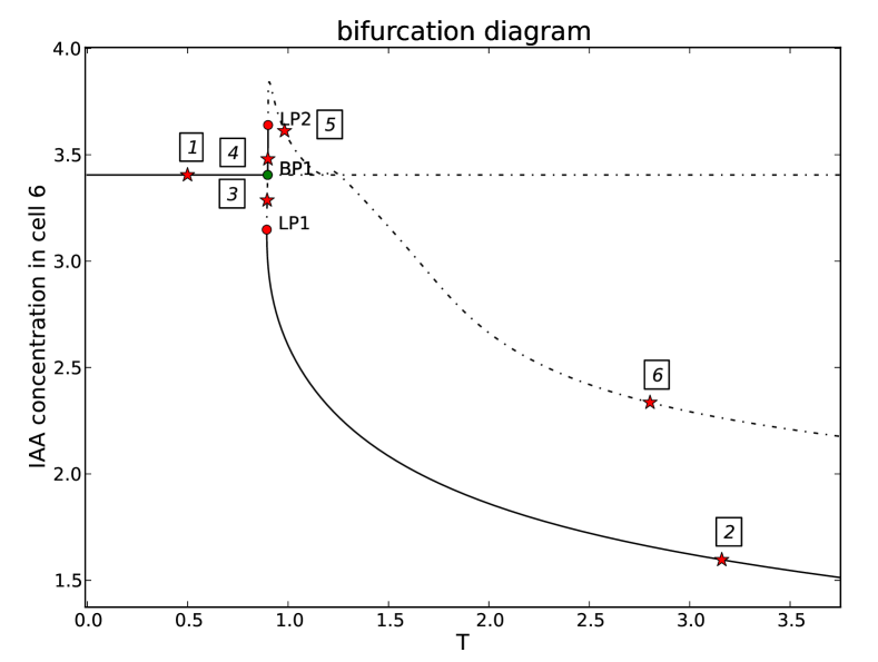
(a) Bifurcation Diagram

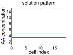
(b) Solution 1

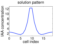
(c) Solution 2

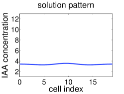
(d) Solution 3

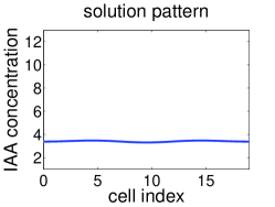
(e) Solution 4

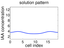
(f) Solution 5

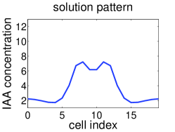
(g) Solution 6

Figure 7: (a) The bifurcation diagram of example 1 (steady state equation (9)) for a row of $20$ cells with the IAA concentration in cell number 6 versus the continuation parameter T (IAA transport coefficient). Other parameters are taken from M1. BP denotes a branch point and LP a limit point. The stars mark the places of the figures displayed below.
(b)-(g) On these figures the IAA concentration in the whole domain is displayed corresponding with the stars marked on (a).

Figure 7a shows the bifurcation diagram that depicts the concentration of auxin in cell number 6 versus the parameter T. The other plots in figure 7 show the steady state auxin patterns in all cells for the specific places indicated with labels in the bifurcation diagram.
The trivial solution curve is the starting point of the continuation. It is the flat horizontal line in the bifurcation diagram. When the parameter T becomes larger than a critical value (T$=0.8983$), the trivial solution loses its stability at a branch point. It was found by calculating for every solution $\left(\textbf{U}_{i},\boldsymbol{\lambda}_{i}\right)$ on the branch, the eigenvalues of the augmented Jacobian matrix defined as

$$J_{\text{aug}}=\left[J_{\mathbf{U}}\left|J_{\boldsymbol{\lambda}}\right.\right].$$ (16)

If the Jacobian $J_{\mathbf{U}}$ is singular and the rank of the augmented Jacobian is still smaller than $2n$, then the solution point $\left(\textbf{U}_{i},\boldsymbol{\lambda}_{i}\right)$ is a branch point. This means that there exist an eigenvalue $\mu\left(\boldsymbol{\lambda}_{i}\right)$ of the Jacobian which is equal to zero. Inserted into a graph, there is a path of an eigenvalue of the solution points corresponding to $\boldsymbol{\lambda}$ close to $\boldsymbol{\lambda}_{i}$, that crosses the imaginary axis at the real axis when $\boldsymbol{\lambda}=\boldsymbol{\lambda}_{i}$. In the branch point on figure 7 there is an exchange of stability to another branch, also shown in the diagram. There are two stable parts on this other solution branch with patterns. When the IAA transport coefficient T is large, the stable solution pattern on this branch consist of one big peak (figure 7c). The other stable part on this branch appears in a very limited range where T is smaller. For example solution 4 is such a stable pattern and it has two small variations (figure 7e). The pattern in figure 7c is the same pattern that was obtained by numerical integration with the fourth order Runge-Kutta in figure 4 as discussed in Section 2.2. We thus found a connection between the trivial flat solution and the numerical solution with peaks.

Example 2.

Here we illustrate a second scenario in which the trivial solution loses its stability. It describes the results of the bifurcation analysis for the model with parameter set M2 that Smith et al. used in their publication (Smith et al, 2006). It differs from the parameter set M1 by a lower production coefficient of IAA, $\rho_{{}_{\textnormal{{\tiny IAA}}}}$. In the previous example, the stability was lost in a branch point. Now, we find that the stability is lost through a Hopf bifurcation where the equilibrium transitions into a periodic orbit. Looking at the eigenvalues of the Jacobian in this Hopf point, there is a pair of eigenvalues that satisfies

$$\mu\left(\boldsymbol{\lambda}_{i}\right)=\pm i\beta.$$ (17)

If we draw a trajectory of the eigenvalues of solution points with $\boldsymbol{\lambda}$ close to $\boldsymbol{\lambda}_{i}$, we see that there are two complex conjugated eigenvalues different from zero that cross the imaginary axis when $\boldsymbol{\lambda}=\boldsymbol{\lambda}_{i}$.

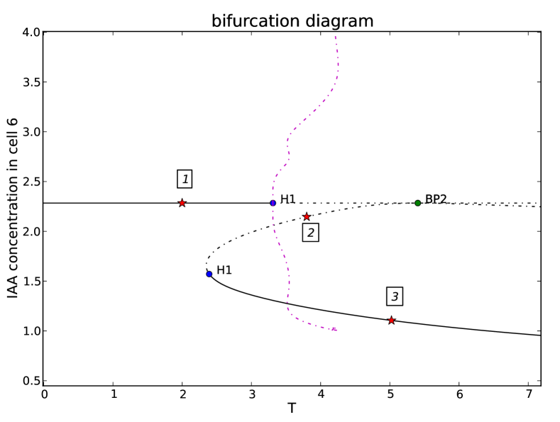
(a) Bifurcation Diagram

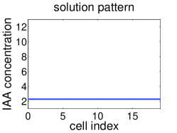
(b) Solution 1

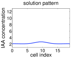
(c) Solution 2

(d) Solution 3

Figure 8: (a) The bifurcation diagram of example 2 (steady state equation (9)) for a row of $20$ cells with the IAA concentration in cell number $6$ versus the continuation parameter T (IAA transport coefficient). Other parameters are taken from M2. The stars mark the places of the figures displayed below. The dotted line through point H1 shows the maximal and minimal value of the IAA concentration in cell number 6 of the periodic solution for each choice of the parameter T. H and BP denote respectively a Hopf point and a branch point.
(b)-(d) On these figures the IAA concentration in the whole domain is displayed corresponding with the stars marked on (a).

Figure 8a shows the bifurcation diagram depicting again the concentration of IAA in cell $6$ versus the continuation parameter T for the same model as in example 1, but now for parameter set M2. In this situation, the stability of the trivial solution is lost in a Hopf point at T $=3.3113$. The branch that emerges from this Hopf point, shows the maximal and minimal IAA concentration over the orbit for each choice of parameter T. All the solutions on this branch are unstable and therefore we only have unstable periodic solutions. Further, also another steady state branch, different from the trivial solution branch, is displayed. This branch intersects with the trivial solution branch at a branch point (T $=5.4047$ ). Around this branch point, all solutions are unstable. However, when we follow this new branch, we encounter another Hopf point where we now gain stability. The pattern of these stable solutions consist of one single big peak in the middle of the domain (see figure 8d).

Example 3.

This example illustrates that there are stable orbits beyond the Hopf bifurcation point for some particular choices of the parameters. For the third example parameter set M3 is used that differs from sets M1 and M2 in the production coefficient of IAA. It is smaller than in set M2. Again equation (9) is solved.

The resulting bifurcation diagram is shown in figure 9.

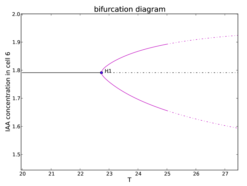
Figure 9: Bifurcation diagram of example 3 where equation (9) was solved with parameter set M3. It depicts the IAA concentration in cell number 6 versus the continuation parameter T (IAA transport coefficient). H denotes a Hopf point. The stable orbit for T$=23.5$ is shown on figure 10.

As in example 2, the stability of the trivial solution is lost in a Hopf point (T $=22.7384$). However, in contrast with this previous example, the periodic solution branch that intersects with the trivial solution branch in this point contains stable periodic solutions. Figure 10 shows, in a three dimensional plot, the stable periodic solution for IAA transport coefficient $T=23.5$ found with RK4 starting from the initial value

$$p_{i}(0)=1.79\quad\text{and}\quad a_{i}(0)=3.76,$$ (18)

where a small perturbation $0.02\sin\left(\left(5\left(i+2\right)\pi\right)/24\right)$ for $i=1,\ldots,20$ was added. Any other initial state nearby will lead to the same long term solution.

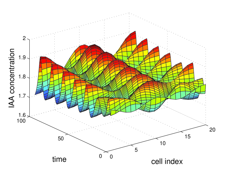
Figure 10: The time evolution of equations (1), (1.2.2) and (3) for a row of $20$ cells starting from the initial value in equation (18) and with parameter set M3 but with IAA transport coefficient T$=23.5$. We used RK4 for numerical integration. The resulting solution is a periodic solution where the pattern changes from one peak concentration of auxin in the middle of the domain to a pattern with high concentrations at the boundaries. The periodic solution corresponds with the solution for T$=23.5$ on the periodic solution branch in figure 9.

We see that the periodic solution changes in time from a pattern with one peak concentration of auxin in the middle of the domain to a pattern with two high auxin concentrations at the sides of the domain.

Figure 11: The trajectory of the time evolution of figure 10 in the $\left(a_{6}\left(t\right),da_{6}\left(t\right)/dt\right)$-plane. We used a row of $20$ cells starting from initial value (18) and parameter set M3 but with IAA transport coefficient T$=23.5$ and we used RK4 for numerical integration.

In figure 11 we plotted this trajectory in the $\left(a_{6}\left(t\right),da_{6}\left(t\right)/dt\right)$-plane starting from the initial value in equation (18).

Example 4.

The previous three examples showed a part of the bifurcation diagrams for equation (9) corresponding with parameter sets M1, M2 and M3, that differ in IAA production rate, for a one dimensional domain of 20 cells. In this example we look to a row of $100$ cells and use the parameter values of set M1. In this example, the stability of the trivial solution is again, as in example 1, lost at a branch point (T $=0.8504$) (see figure 12a). The branch that crosses the trivial solution branch in this point is a bit more complicated. The branch contains 3 different stable parts.

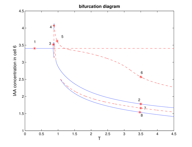
(a) Bifurcation Diagram

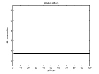
(b) Solution 1

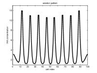
(c) Solution 2

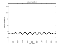
(d) Solution 3

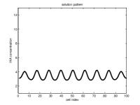
(e) Solution 4

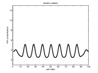
(f) Solution 5

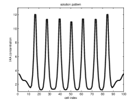
(g) Solution 6

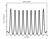
(h) Solution 7

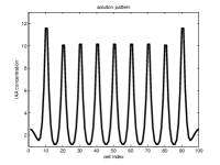
(i) Solution 8

Figure 12: (a) Bifurcation diagram of example 4 (steady state equation (9)) for a row of $100$ cells and parameter set M1. The diagram shows the IAA concentration in cell number $6$ versus the continuation parameter T (IAA transport coefficient). The unconnected branch is found by time integrating the steady state solution of figure 7c copied five times in a row until a steady state is found. The resulting steady state is then used as a starting point for the continuation.The stars mark the places of the figures displayed below. (b)-(i) On these figures the IAA concentration in the whole domain is displayed corresponding with the stars marked on (a).

The stable part that contains solution point 2 consists of solutions with a pattern with 8 peaks (see figure 12c). Also the small stable area on the branch that contains solution 3 consists of patterns with $8$ peaks, but they are smaller due to the small value of T in this region. We see that the peaks become higher for an increasing IAA transport coefficient T (compare for example the patterns in figures 12c and 12d or in figures 12f and 12g). The third stable part on this solution branch, appears also in a limited range of T. The patterns show only $7$ peaks of high auxin concentration (see figure 12e). The patterns on the unstable part of the branch that contains solutions $5$ and $6$ also consist of 7 peaks (see figure 12f and 12g)

The other solution branch in figure 12a is found by time integration by starting with the steady state solution of figure 4 or the pattern in figure 7c copied five times in a row which rapidly leads to a steady state that can be used as a starting point for the continuation. We see that this branch is not (directly) linked with the trivial solution branch and consists of one stable and one unstable part. On both parts the patterns consist of $9$ high peaks of auxin concentration (see figures 12h and 12i).

Figures 7, 8, 9 and 12 for examples 1, 2, 3 and 4 show different bifurcation diagrams of equation (9). In the examples 1 and 4, where parameter set M1 is used, the stability of the trivial solution is lost in a branch point. While in the examples 2 and 3 it is lost in a Hopf point. We can calculate the type of these bifurcation points for every transition from stable to unstable for the three dimensional space of the parameters D, T and $\rho_{{}_{\textnormal{{\tiny IAA}}}}$. We found that in the one-dimensional case, for a row of cells, only two different situations can occur: either the stability of the trivial solution is lost in a Hopf point or it is lost in a branch point. Figure 13 shows, for a row of $20$ cells and parameter values from table 1, the stability boundary for the parameters D, T and $\rho_{{}_{\textnormal{{\tiny IAA}}}}$. The line also indicates the corresponding type of bifurcation.

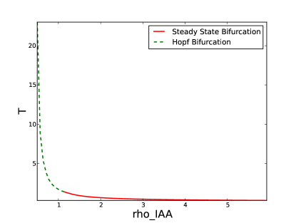
(a) $\textrm{D}=1.000$

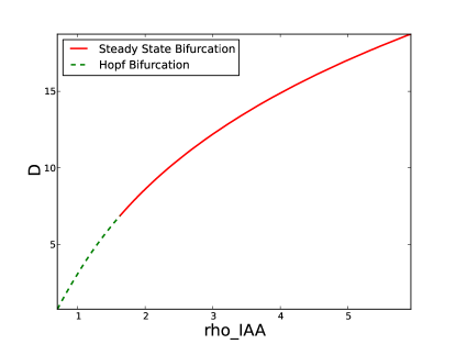
(b) $\textrm{T}=3.500$

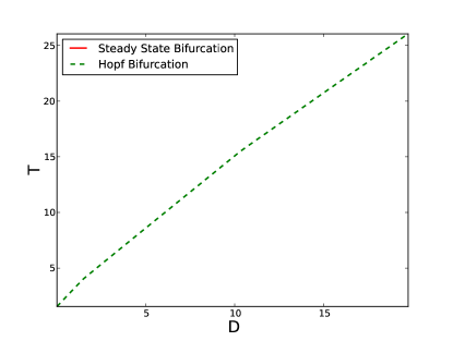
(c) $\rho_{{}_{\textnormal{{\tiny IAA}}}}=0.750$

Figure 13: Map of types of bifurcation points for equation (9) and a row of $20$ cells and different choices of the parameters $\rho_{{}_{\textnormal{{\tiny IAA}}}}$ (IAA production coefficient), D (IAA diffusion coefficient), T (IAA transport coefficient). Other parameters are taken from table 1.

For example figure 13a shows that for small values of the production coefficient of IAA the stability of the trivial solution will be lost in a Hopf point. Indeed, in example 2 and 3 we found similar results.

Example 5.

This example explores the role of the quadratic dependence of the active transport on the auxin concentration and the bifurcation diagrams will be calculated for varying exponents $\tau$. We will use the adapted model with active transport equation (6) with parameter $\omega$ equal to one and for different values for parameter $\tau$. The results in figure 14 show the concentration of auxin in cell number $6$ versus the parameter T for $\tau=1/2,1,3/2$ and $2$. In this example we use again parameter set M1 and a row of $20$ cells, as in example $1$.

Figure 14: The bifurcation diagrams of example 5 for a row of $20$ cells with the IAA concentration in cell number $6$ versus the continuation parameter T (IAA transport coefficient). The adapted model with active transport equation (6) is used where the exponent in the active transport ($\tau$) is set to different values ($\tau=2,3/2,1$ and $1/2$). The parameter $\omega$ is set to 1 and the other parameter values are taken from M1.

The flat branch, on top of the figure, is the trivial solution branch, which is independent of the value for the exponent $\tau$. However, the stability of this branch depends on $\tau$ and is only shown for $\tau=1/2$.

Similarly to example 1 the trivial solution loses, for each choice of $\tau$, its stability at a branch point. These points are indicated on the trivial solution branch with a dot for $\tau$ equal to $1/2,1,3/2$ and $2$ (left to right in the figure), where the latter is the model of Smith and co-authors. The larger $\tau$, the more the bifurcation point shifts to the right. Thus the stability of the trivial solution is lost for larger values of the transport coefficient T. This result corresponds with the result in section 3.1.

The branches that emerge at these points contain steady state solutions with peaks as described earlier. Note that figure 14 only shows the bottom half of the emerging branches. The branch at the right with $\tau=2$ contains the solutions with peaks for the model with exponent 2 and is the basic coupled model of Smith et al.. This branch is the same branch as in figure 7a. For other choices of the exponents the figure is qualitatively the same. Only the stability changes slightly. When $\tau$ is smaller the range of transport coefficients T where the solution branch is stable becomes smaller.

We have also found that the spacing between the peaks hardly changes if $\tau$ is changed in a continuous way

So we conclude that there is little difference between the quadratic or linear dependence of the active transport on the auxin concentration. Varying the exponent leads to qualitatively the same bifurcation.

Example 6.

This example explores the influence of the exponential dependence of the localization of PIN1 on the concentration of IAA. We change, in a continuous way, the parameter $\omega$ in the active transport equation (6). Figure 15 shows the bifurcation diagram that depicts the concentration of auxin in cell number 6 versus the parameter $\omega$ for parameter set M1 and a row of $20$ cells. The transport coefficient T is now fixed at $1.5$.

Figure 15: The bifurcation diagram of example $6$ for a row of $20$ cells, parameter set M1 and active transport equation (6) with $\tau=2$. The diagram shows the IAA concentration in cell number $6$ versus the continuation parameter $\omega$. The flat branch is the trivial solution, the other branch is found by starting with the steady state solution found in section 2.2 for $\omega=1$.

Again the flat branch represents the trivial solution that is independent of the parameter $\omega$. When $\omega$ is equal to zero, the active transport equation is equal to equation (5) and here the trivial solution is stable (see also in section 3.1). When $\omega$ increases, and the model transitions into the basic coupled model of Smith et al., the trivial solution becomes unstable (at $\omega=0.2371$). The other branch on this figure contains steady state solutions with peaks. For $\omega$ equal to one, the solution corresponds with the steady state solution in figure 4. When $\omega$ becomes smaller, the solution with peaks loses its stability in a turning point ($\omega=0.1424$). The solution with peaks of figure 4 in the model with $\omega=1$ has no corresponding solution in the model with $\omega=0$. This bifurcation diagram shows only a connection between the model with $\omega=0$ and $\omega=1$ by the trivial solution.

Similar figures are found for other choices of the transport coefficient $T$.

6 Conclusion and discussion

In this paper we explored the model proposed by Smith et al (2006) for the transport of auxin in a one-dimensional row of cells. The model describes the evolution of the concentration of PIN1 and IAA in each of the cells by a coupled set of non-linear ordinary differential equations. The change in concentration of IAA in each cell depends only on PIN1 and IAA concentrations in that cell, its nearest and next-nearest neighbors and this leads to a sparsely coupled system.

We analyzed the steady state solutions of the system as a function of three of the 11 parameters in the problem. We have varied the IAA transport coefficient T, the diffusion coefficient D and the production rate $\rho_{\textnormal{{\tiny IAA}}}$. Furthermore, we introduced a slight generalization of the active transport equation. The main tool used in the paper is numerical continuation to generate these solutions starting from a trivial solution of the system.

The trivial solution is identified as an analytical solution where the concentration in all the cells is the same. This solution is stable for some region of the parameter space. However, changing the parameters, for example, increasing the IAA transport coefficient T, destroys its stability. In contrast to the uncoupled system studied by Jönsson et al (2006), the eigenvalues of the Jacobian of this coupled system can not be easily analyzed analytically. The Jacobian now has a blocked sparse structure and its eigenvalues are studied numerically.

In the exploration of the solutions, we identified two generic bifurcation scenarios through which the trivial solution loses its stability. These scenarios reappear for various choices of the parameters. In the first scenario, a stable solution can lose its stability through a branch point, where it becomes a pattern with regular spaced peaks of high auxin concentration. This solution was already found by Smith and collaborators by direct numerical simulation. The spacing and the height of the peaks in the pattern depends on the other parameters of the system.

However, we have found in the coupled system that the trivial state can also lose it stability through a Hopf bifurcation, where the Jacobian has two complex conjugate eigenvalues that become purely imaginary. For a limited parameter range this leads to stable periodic solutions, where the concentration in the cell changes periodically over time. However, for another range of parameters these periodic orbits are unstable and the trivial solution then loses its stability through an unstable orbit. The steady state solution then falls, beyond a parameter threshold, back to a pattern of regularly spaced peaks (see figure 8). These Hopf bifurcation and the periodic solutions are not present in the model studied by Jönsson where the PIN1 concentration is kept constant and all eigenvalues of the Jacobian are real.

These are the only two bifurcation scenarios that we have found at the stability boundary of the trivial solution for various choices of the 11 parameters in the model and for an increasing number of cells in the row.

We also explored modifications to the model of the active transport. The quadratic dependence on the auxin concentration is replaced by a linear dependence. The resulting bifurcation diagram is qualitatively the same. However, replacing the exponential dependence of the pin localization on the auxin transport leads to a different dynamical system where the trivial solution is always stable.

Although the paper studies the steady state solutions of a rather academic model with a row of equal sized square cells, the authors believe it is a valuable contribution to our understanding of pattern formation by auxin accumulation since it builds the foundation for a rigorous bifurcation analysis of the steady state patterns in a two dimensional array of cells.

As demonstrated by Smith et al (2006) generalized linear models are a powerful first step to understand the behavior of the biological system. Such studies can be complemented by simulations of patterns of higher complexity that more closely resemble specific biological systems.

Applying the numerical continuation framework to a more general network of connected (ir)regular shaped cells, requires a Newton-Krylov solver so that the Newton iteration deals with the non-linearity and the Krylov iteration solves the Jacobian system exploiting the sparsity. Furthermore the Krylov subspace iteration only requires the application of the Jacobian to a vector, which avoids the explicit construction of the Jacobian matrix (Kelley, 1995).

For the two dimensional array of cells, we expect to find a similar trivial solution that will lose again its stability as the parameters change and turn into regular patterns of high concentration peaks and time periodic solutions.

In this paper we, essentially re-implemented the same linear file of cells as Smith et al (2006), but instead of using wrap-around boundary conditions, we implemented homogeneous Neumann boundary conditions. In principle it is also possible to investigate the effect of varying in- and out-flux from the system and performing similar studies for these inhomogeneous Neumann boundary conditions. However, then there is no analytically solvable trivial solution.

There are several situations where changing boundary conditions are biologically relevant. First, in the leaf mesophyll, where a row of cells in which local maxima may induce new vascular development could be located between margins. These are a possible source of auxin and emerging veins that drain the auxin (Scarpella et al, 2006), or at a later stage be surrounded by veins draining locally produced auxin. Second, in epidermal cells at the shoot apex along a tip to base gradient, where auxin comes in from the base and is transported to apical positions. And finally, in central linear cell files in the root, auxin flows from base to tip and in the external layers auxin flows from the tip to the base leading to auxin gradients (Grieneisen et al, 2007).

We have explored continuation in the Neumann boundary condition and found, amongst others, s-shaped bifurcation diagrams with double limit points. This leads to a hysteresis effect in the boundary conditions. This is described in Draelants et al (2012).

Also for problems with periodic boundary conditions a similar analysis can be performed. There, however, the Jacobian will have a one dimensional null-space associated with the translation invariance of solutions. This can be regularized by introducing a phase condition as described by (Champneys and Sandstede, 2007).

There are still many uncertainties in the current generation of models. Especially the large number of parameters and the uncertainty in their values is a reason for concern. By focusing on the qualitative properties of the transitions that appear in the models rather than on the states for particular choices of the parameters, we hope to understand more about the possible patterns that appear in real systems. It is valuable to calculate similar bifurcation diagrams for all the proposed models for auxin transport using the numerical continuation methods. We could also use homotopy and use a continuous transformation to go from one model into another model. Numerical continuation can then follow the solutions from one model into the solutions of another model. This will allow the comparison of models across a range of parameters and check if they exhibit qualitatively the same transition if parameters change.

In real plants it is impossible to tune a parameter such as the transport coefficient T in a continuous way as is done in these calculations. It can only be changed in discrete steps in a plant by the introduction of, for example, mutations that compromise or enhance the auxin production or transport. Comparing such experiments with the model outcome will make it possible to refine the models to give a more realistic description of the biological system.

The bifurcation analysis on the linear system with zero-influx at the boundaries yields interesting new insights into the potential behaviors of the biological system. It is interesting to note that low values of the IAA transport coefficient lead to flat distributions of the auxin concentration, whereas high concentrations are required to establish sharp accumulation peaks.

1-N-naphthylphthalamic acid (NPA) has long been used experimentally as an inhibitor of auxin efflux. The precise molecular mechanism by which NPA impacts on auxin transport is still unknown, although several NPA-binding proteins have been identified (Muday and Delong, 2001). Previously, we have assumed that NPA inhibits the cycling of PIN proteins to the cell membrane (Merks et al, 2007). In terms of our model, this would relate to a lowering of $\rho_{{}_{\textnormal{{\tiny PIN}}_{0}}}$ and/or $\rho_{{}_{\textnormal{{\tiny PIN}}}}$ which results in the formation of lower auxin peaks. Indeed, experimental inhibition of auxin transport with NPA abolishes the normal narrow accumulation peaks and results in a much flatter auxin distribution pattern (Scarpella et al, 2006). Also consistently with the model, the vam3 mutation that perturbs PIN1 polarization, prevents auxin peaks forming and inhibits formation of higher order veins (Shirakawa et al, 2009). More recently it was shown that a mutation in the auxin import carrier lax2, which inhibits auxin transport increases the numbers of vascular strand breaks (Péret et al, 2012), which may also be explained by the model prediction of lower auxin maxima, which could be unable to fully induce vascular development. Thus, the model behavior appears to be consistent with physiological treatments and mutations that affect specific model parameters.

The bifurcation analysis also yields interesting new insights into additional potential behaviors of the biological system. One especially interesting behavior is the oscillation obtained with a specific set of parameter values (Fig 10). This behavior has to our knowledge never been observed in the context of leaf development. However, in the root basal meristem, oscillating auxin concentrations have been observed and related to the regular induction of laterals along the growing axis of the root (De Smet et al, 2007).

One other characteristic unveiled by the bifurcation analysis is that across the region where a pattern of auxin accumulation peaks are generated, these peaks occur at very stable distances. This would imply that in the case of vascular patterning, the initial distance between veins is relatively stable, implying that observed differences in vascular density in mature leaves (Dhondt et al, 2011) largely result from differences in subsequent development. This is an example of an new hypothesis generated by modeling a biological process that can be experimentally validated and underlines the importance of systematic exploration of biologically relevant parameter variations.

It is important to repeat that we have kept the plant geometry fixed in the current model. It is an open question how the calculations can be extended to include cells to undergo growth and division.

References

- Allgower and Georg (1994) Allgower E, Georg K (1994) Numerical Path Following. Springer-Verlag Berlin
- Benková et al (2003) Benková E, Michniewicz M, Sauer M, Teichmann T, Seifertová D, Jürgens G, Friml J (2003) Local, efflux-dependent auxin gradients as a common module for plant organ formation. Cell 115:591–602
- Bilsborough et al (2011) Bilsborough G, Runions A, Barkoulas M, Jenkins H, Hasson A, Galinha C, Laufs P, Hay A, Prusinkiewicz P, Tsiantis M (2011) Model for the regulation of arabidopsis thaliana leaf margin development. Proceedings of the National Academy of Sciences 108:3424–3429
- Champneys and Sandstede (2007) Champneys A R and Sandstede B (2007) Numerical computation of coherent structures. In: Numerical Continuation Methods for Dynamical Systems (Edited by B Krauskopf, HM Osinga and J Galan-Vioque). Springer 331–358
- Clewley et al (2007) Clewley R, Sherwood W, LaMar M, Guckenheimer J (2007) Pydstool, a software environment for dynamical systems modeling. url http://pydstool.sourceforge.net
- De Smet et al (2007) De Smet I, Tetsumura T, De Rybel B, Frey N, Laplaze L, Casimiro I, Swarup R, Naudts M, Vanneste S, Audenaert D, Inzé D, Bennet M, Beeckman T (2007) Auxin-dependent regulation of lateral root positioning in the basal meristem of arabidopsis. Development 134:681–690
- Dhondt et al (2011) Dhondt S, Van Haerenborgh D, Van Cauwenbergh C, Merks R, Philips W, Beemster G, Inzé D (2011) Quantitative analysis of venation patterns of arabidopsis leaves by supervised image analysis. The plant Journal 69:553–563
- Doedel et al (1997) Doedel E, Champneys A, Fairgrieve T, Kuznetsov Y, Sandstede B, Wang X (1997) Continuation and bifurcation software for ordinary differential equations (with homcont). Available by anonymous ftp from ftp cs concordia ca, directory pub/doedel/auto
- Draelants et al (2012) Draelants D, Vanroose W, Broeckhove J, Beemster G T S, Influence of an exogenous model parameter on the steady states in an auxin transport model. Submitted 2012.
- Grieneisen et al (2007) Grieneisen V A, Xu J, Marée A F M, Hogeweg P, Scheres B (2007) Auxin transport is sufficient to generate a maximum and gradient guiding root growth. Nature 449:1008–1013
- Hairer et al (2009) Hairer E, Nørsett S, Wanner G (2009) Solving ordinary differential equations I : nonstiff problems. Springer
- Hoyle (2006) Hoyle R B , (2006) Pattern formation: an introduction to methods. Cambridge University Press.
- Jönsson et al (2006) Jönsson H, Heisler M, Shapiro B, Meyerowitz E, Mjolsness E (2006) An auxin-driven polarized transport model for phyllotaxis. PNAS 103(5):1633–1638
- Kelley (1995) Kelley, C.T. (1995) Iterative methods for linear and nonlinear equations, Society for Industrial Mathematics
- Krauskopf et al (2007) Krauskopf B, Osinga H, Galán-Vioque J (2007) Numerical continuation methods for dynamical systems: path following and boundary value problems. Springer Verlag
- Merks et al (2007) Merks R M H, Van de Peer Y, Inzé D, Beemster G T S (2007) Canalization without flux sensors: a traveling-wave hypothesis. Trends in Plant Science 12, 384-390
- Muday and Delong (2001) Muday G K and DeLong A (2001) Polar auxin transport: controlling where and how much. Trends Plant Sci. 6, 535–542
- Palme and Gälweiler (1999) Palme K, Gälweiler L (1999) Pin-pointing the molecular basis of auxin transport. Current Opinion in Plant Biology 2(5):375–381
- Péret et al (2012) Péret B, Swarup K, Ferguson A, Seth M, Yang Y, Dhondt S, James N, Casimiro I, Perry P, Syed A, Yang H, Reemer J, Venison E, Howell C, Perez-Amador M A, Yun J, Alonso J, Beemster G T S, Laplaze L, Murphy A, Bennett M J, Nielsen E, Swarup R. AUX/LAX genes encode a family of auxin influx transporters that perform distinct function during Arabidopsis development. Submitted to Plant Cell in 2012.
- Reinhardt et al (2003) Reinhardt D, Pesce E, Stieger P, Mandel T, Baltensperger K, Bennett M, Traas J, Friml J, Kuhlemeier C (2003) Regulation of phyllotaxis by polar auxin transport. Nature 426(6964):255–260
- Salinger et al (2005) Salinger A, Burroughs E, Pawlowski R, Phipps E, Romero L (2005) Bifurcation tracking algorithms and software for large scale applications. International Journal of Bifurcation Chaos in Applied Sciences and Engineering 15(3):1015–1032
- Scarpella et al (2006) Scarpella E, Marcos D, Friml J, Berleth T (2006) Control of leaf vascular patterning by polar auxin transport. Genes & Development 20:1015–1027
- Seydel (1994) Seydel R (1994) Practical bifurcation and stability analysis: from equilibrium to chaos, vol 5. Springer
- Shirakawa et al (2009) Shirakawa M, Ueda H, Shimada T, Nishiyama C, Hara-Nishimura I (2009) Vacuolar SNAREs function in the formation of the leaf vascular network by regulating auxin distribution. Plant & Cell Physiology 50(7):1319–1328.
- Smith et al (2006) Smith R, Guyomarc’h S, Mandel T, Reinhardt D, Kuhlemeier C, Prusinkiewicz P (2006) A plausible model of phyllotaxis. PNAS 103(5):1301–1306