Transport properties of anisotropically expanding quark-gluon plasma within a quasi-particle model

Abstract

The bulk and shear viscosities ($\eta$ and $\zeta$) have been studied for quark-gluon-plasma produced in relativistic heavy ion collisions within semi-classical transport theory, in a recently proposed quasi-particle model of (2+1)-flavor lattice QCD equation of state. These transport parameters have been found to be highly sensitive to the interactions present in hot QCD. Contributions to the transport coefficients from both the gluonic sector and the matter sector have been investigated. The matter sector is found to be significantly dominating over the gluonic sector, in both the cases of $\eta$ and $\zeta$. The temperature dependences of the quantities, $\zeta/{\mathcal{S}}$, and $\zeta/\eta$ indicate a sharply rising trend for the $\zeta$, closer to the QCD transition temperature. Both $\eta$, and $\zeta$ are shown to be equally significant for the temperatures that are accessible in the relativistic heavy ion collision experiments, and hence play crucial role while investigating the properties of the quark-gluon plasma.

PACS: 25.75.-q; 24.85.+p; 05.20.Dd; 12.38.Mh

Keywords: Transport coefficients; Shear viscosity; Bulk viscosity; Quasi-particle model; Effective fugacity; Transport theory; Chromo-Weibel instability.

I Introduction

The study of transport coefficients for hot QCD matter is an area of intense research since the discovery of a fluid like picture of quark-gluon-plasma (QGP) in the relativistic heavy ion collider (RHIC) at BNL expt . The discovery of the QGP is attributed to the fact that at extreme energy-density and temperature, ordinary nuclear matter goes through a transition to the QGP phase as predicted by the finite temperature Quantum-Chromodynamics (QCD) (this transition is shown to be a crossover cross at the vanishing baryon density).

To describe a fluid, shear and bulk viscosities ($\eta$ and $\zeta$ respectively) are very important physical quantities that characterize dissipative processes during its hydrodynamic evolution. The former describes the entropy production due to the transformation of the shape of hydrodynamic system at a constant volume, and the latter describes the entropy production at the constant rate of change of the volume of the system (hot fireball at the RHIC). Moreover, $\eta/{\mathcal{S}}$, and $\zeta/{\mathcal{S}}$ serve as the inputs while studying the hydrodynamic evolution of the fluid shrhydro ; bulkhydro . One can also couple hydrodynamics with the Boltzmann descriptions at the later stages after the collisions of heavy ions at the RHIC, by maintaining the continuity of the entire stress energy tensor and currents. The process could be translated in terms of the viscous modifications to the thermal distributions functions of particles. This leads to a smooth transition from the hydrodynamic regime where the mean free paths are short to a region where hydrodynamics is inapplicable and Boltzmann treatments seems to be justified prat . Therefore, this sets a way to study the impact of transport coefficients of the QGP in various processes at the RHIC, and the ongoing heavy ion experiments at Large Hadron Collider (LHC), CERN (e.g. dilepton production, quarkonia physics etc.). Regarding viscous corrections to dilepton production rate at the RHIC, we refer the reader to  srikanth . The determinations of $\eta$ and $\zeta$ have to be done separately from a microscopic theory; either from a transport equation landau with an appropriate force, collision, and source terms or equivalently from the field theoretic approach by employing the Green-Kubo formulas green-kubo (long wavelength behavior of the correlations among various components of the stress-energy tensor).

The QGP is strongly interacting at the RHIC expt , as inferred from the flow measurements, and strong jet quenching observed there. This observation is found to be consistent with the lattice simulations of the hot QCD equation of state (EOS) leos_lat ; leos1_lat , which predict a strongly interacting behavior even at temperatures which are of the order of a few $T_{c}$ (the QCD transition temperature). The flow measurements suggest a very tiny value for the ratio of $\eta$ to the entropy density, ${\mathcal{S}}$ ($\eta/{\mathcal{S}}$) for the QGP, and the near perfect fluid picture shrvis ; bmuller ; chandra_eta1 ; chandra_eta2 (except near the QCD transition temperature where $\zeta/{\mathcal{S}}$ is equally significant as $\eta/{\mathcal{S}}$ khaz ; mayer ; buch ; chandra_bulk ).

Preliminary studies at the LHC alice ; alice1 ; hirano reconfirm above mentioned observations regarding the QGP. In heavy-ion collisions at the LHC, in addition to the elliptic flow obtained at the RHIC, there are other interesting flow patterns, viz., the dipolar, and the triangular flow, which are sensitive to the initial collision geometry flow_lhc . There have been recent interesting studies to understand them at LHC bhalerao ; alice . A more precise measurement of various flows and jet quenching at LHC is awaited. On the other hand, $\zeta$ has achieved considerable attention in the context of the QGP after the interesting reports on its rising value close to the QCD transition temperature khaz . Subsequently, the possible impact of the large bulk viscosity of the QGP at the RHIC have been studied by several authors; Song and Heinz heinz have studied the interplay of shear and bulk viscosities in the context of collective flow in heavy ion collisions. Their study revealed that one can not simply ignore the bulk viscosity while modeling the QGP. In this context, there are other interesting studies in the literature den ; raj1 ; hirano1 ; raj ; efaaf ; pion ; fries . The role of bulk viscosity in freeze out phenomenon has been offered in torri ; hirano . Effects of bulk viscosity in the hadronic phase, and in the hadron emission have been studied in boz . Interestingly, in the recent investigations, these transport coefficients are found to be very sensitive to the interactions chandra_eta1 ; chandra_eta2 , and the nature of the phase transition in QCD moore . Another crucial aspect of $\zeta$ is its influence on the domain of applicability of hydrodynamics at the RHIC, viz. the phenomenon cavitation. This phenomenon has been addressed in detail in the context of diverging value of $\zeta$ near the QCD transition temperature in rajgopal ; srikanth1 . Thus, the determinations of $\eta$ and $\zeta$ for the QGP have multi-facet dimensions, and significant impact on the variety of physical phenomena at the RHIC and the LHC. Subsequently, the cavitation in a particular string theory model (N=2* SU(N) theory which is non-conformal, and mass deformation of N=4, SU(4) Yang-Mills) has been investigated by Klimek, Leblond, and Sinha in sinha . They have observed the absence of cavitation before phase transition is reached, by investigating the flow equations in (1+1)- dimensional boost invariant set up, which is in contrast to the finding of rajgopal for hot QCD. They further argued that such a behavior is mainly due to to smaller value of $\zeta$, and sharp rise of the relaxation time for such theories near the transition point, and perhaps the quantum corrections to $\eta$, and $\zeta$ sinha_qnt . These studies might play a crucial role in understanding the behavior of strongly coupled QGP (sQGP) in the RHIC and the LHC.

The determinations of $\eta$ and $\zeta$ have been performed adopting the view-point based on the inference drawn from the experimental results, and the lattice QCD (the best known non-perturbative technique to address the QGP). Lattice QCD has indeed been very successful to study the QGP thermodynamics. However, the the computation of the transport coefficients in lattice QCD is a very non-trivial exercise, due to several uncertainties and inadequacy in their determination. Despite that there are a few first results computed from lattice QCD for bulk and shear viscosities meyer ; tmr ; meyer1 ; nakamura which have observed a small value of $\eta/{\mathcal{S}}$, and large $\zeta/{\mathcal{S}}$ at the RHIC. A very recent interesting analysis gupta suggests that it is possible to compare the direct lattice results with the experiments at the RHIC. From such a comparison, the QCD transition temperature came out to be around $175MeV$. More refined lattice studies on $\eta$ and $\zeta$ are awaited in the near future.

The work presented in this paper is an attempt to achieve, (i) temperature dependence of $\eta$ and $\zeta$ (The gluonic as well as the matter sector contributions to these transport parameters have been obtained by combing a transport equation with a recently proposed quasi-particle model chandra1 ; chandra2 ; chandra_quasi of $(2+1)$-flavor lattice QCD EOS. Noteworthy point is that the matter sector has largely been ignored in the literature in this context), (ii) to understand the small $\eta/{\mathcal{S}}$, and large $\zeta/{\mathcal{S}}$ for the QGP for the temperatures closer to $T_{c}$. More precisely, inputs has been taken from the computations of $\eta$ and $\zeta$ in quasi-particle models chandra_eta1 ; chandra_eta2 ; kapu ; sakai ; chandra_bulk , and combine the understanding with a transport theory determination of them in the presence of chromo-Weibel instabilities bmuller ; chromw ; bmuller1 . The present work is the extension of our recent work on $\eta$ chandra_eta1 ; chandra_eta2 , and $\zeta$ chandra_bulk for the gluonic sector, to the (2+1)-flavor QCD.

The paper is organized as follows. In Sec. II, we present the formalism to compute the $\eta$ and $\zeta$. The quasi-particle model and transport equation have also been discussed in brief in the same section. In Sec. III, we have presented the results on the temperature dependence of $\eta$ and $\zeta$ in $(2+1)$-flavor lattice QCD, and relevant physics. In Sec. IV, we have presented conclusions and future prospects of the present work.

II Determination of transport coefficients

There may be a variety of physical phenomena that lead to the viscous effects in the QGP (or in general any interacting system)  prat . Among them, our particular focus is on the viscous effects which get contributions from the the classical chromo-fields.

The idea adopted here is based on the mechanism earlier proposed in  bmuller ; bmuller1 ; majumdar to explain the small viscosity of a weakly coupled, but expanding QGP. The mechanism in the context of the QGP is solely based on the particle transport processes in the turbulent plasmas dupree that are characterized by strongly excited random field modes in the certain regimes of instability. They coherently scatter the charged particles, and thus reduce the rate of momentum transport. This eventually lead to the suppression of the transport coefficients in plasmas. This phenomenon has been studied both in electro-magnetic (EM) plasmas niu , and in non-abelian plasmas (QCD plasma) by Asakawa, Bass and Müller bmuller ; bmuller1 , and further employed for the realistic QGP EOS in chandra_eta1 ; chandra_eta2 .

The condition for the spontaneous formation of turbulent fields can be achieved in EM plasmas with an anisotropic momentum distribution weibel of charged particles, and in the QGP with anisotropic distribution of thermal partons sma . In the context of pure SU(3) gauge theory, this mechanism turn out to be successful to explain small shear viscosity of the QGP and larger bulk viscosity for the temperatures accessible at the RHIC and the LHC chandra_eta2 ; chandra_bulk . Here, extension has been desired to the case of realistic EOS for the QGP by incorporating the effects from the matter sector (quark-antiquarks).

It will be seen later that the analysis leads to an interesting observation regarding the relative contribution of the gluonic and the matter sectors to the transport parameters. Before, we present a brief description of the quasi-particle understanding of $(2+1)$-flavor lattice QCD that furnishes an appropriate modeling of equilibrium state.

II.1 The quasi-particle description of hot QCD

Quasi-particle description of the hot QCD medium effects, is not a new concept. There have been several attempts so far to understand the hot QCD medium effects in terms of non-interacting/weakly interacting quasi-partons, viz., effective thermal mass models pesh ; pesh1 , effective mass model with temperature dependent bag parameter to cure the problem of thermodynamic inconsistency pesh1 , effective quasi-particles with gluon condensate glucond , Polyakov loop models polya (Polyakov loop acts as effective fugacity), and the quasi-partons with effective fugacities  chandra1 ; chandra2 ; chandra_quasi . The last one that will be employed here, shown to be fundamentally distinct from all other mentioned models, and in the spirit of Landau’s theory of Fermi liquids. Moreover, the model has been highly successful in interpreting the lattice QCD thermodynamics, and bulk and transport properties of hot QCD matter and the QGP in relativistic heavy ion collisions.

In our quasi-particle description for (2+1)-flavor lattice QCD chandra_quasi , we start with the ansatz that the Lattice QCD EOS can be interpreted in terms of non-interacting quasi-partons having effective fugacities which encode all the interaction effects. We denote them as gluon effective fugacity, $z_{g}$ and the quark-antiquark fugacity, $z_{q}$. In this approach, the hot QCD medium is divided in to two sectors, viz., the effective gluonic sector, and the matter sector (light quark sector, and strange quark sector). The former refers to the contribution of gluonic action to the pressure which also involves contributions from the internal fermion lines. On the other hand, latter involve interactions among quark, anti-quarks, as well as their interactions with gluons. The ansatz can be translated to the form of the equilibrium distribution functions, $f_{eq}\equiv\{f_{g},f_{q},f_{s}\}$ (this notation will be useful later while writing the transport equation in both the sector in compact notations) as follows,

$$f_{g} = \frac{z_{g}\exp(-\beta p)}{\bigg{(}1-z_{g}\exp(-\beta p)\bigg{)}},$$

$$f_{q} = \frac{z_{q}\exp(-\beta p)}{\bigg{(}1+z_{q}\exp(-\beta p)\bigg{)}},$$

$$f_{s} = \frac{z_{q}\exp(-\beta\sqrt{p^{2}+m^{2}})}{\bigg{(}1+z_{q}\exp(-\beta\sqrt{p^{2}+m^{2}})\bigg{)}},$$ (1)

where $m$ denotes the mass of the strange quark, which we choose to be $0.1GeV$. The parameter, $\beta=T^{-1}$ denotes inverse of the temperature. Here, we are working in the units where Boltzmann constant, $K_{B}=1$, $c=1$, and $h/2\pi=1$. The notation $p$ is nothing but, $p\equiv|\vec{p}|$.

We use the notation $\nu_{g}=2(N_{c}^{2}-1)$ for gluonic degrees of freedom , $\nu_{q}=2\times 2\times N_{c}\times 2$ for light quarks, $\nu_{s}=2\times 2\times N_{c}\times 1$ for the strange quark for $SU(N_{c})$. Here, we are dealing with $SU(3)$, so $N_{c}=3$. Since the model is valid in the deconfined phase of QCD (beyond $T_{c}$), therefore, the mass contributions of the light quarks can be neglected as compared to the temperature. Therefore, in our model, we only consider the mass for the strange quarks.

The effective fugacity is not merely a temperature dependent parameter which encodes the hot QCD medium effects. It is very interesting and physically significant. The physical significance reflects in the modified dispersion relation both in the gluonic and matter sector. In this description, the effective fugacities modify the single quasi-parton energy as follows,

$$\omega_{g} = p+T^{2}\partial_{T}ln(z_{g})$$

$$\omega_{q} = p+T^{2}\partial_{T}ln(z_{q})$$

$$\omega_{s} = \sqrt{p^{2}+m^{2}}+T^{2}\partial_{T}ln(z_{q}).$$ (2)

These dispersion relations can be explicated as follows. The single quasi-parton energy not only depends upon its momentum but also gets contribution from the collective excitations of the quasi-partons. The second term is like the gap in the energy-spectrum due to the presence of quasi-particle excitations. This makes the model more in the spirit of the Landau’s theory of Fermi -liquids. For a detailed discussion on the interpretation and physical significance of $z_{g}$, and $z_{q}$, we refer the reader to our recent work chandra_quasi . Henceforth, we shall use gluonic sector in the place of effective gluonic sector for the sake of ease. We shall now proceed to the determination $\eta$ and $\zeta$ in presence of chromo-Weibel instabilities.

II.2 Chromo-Weibel instability and the anomalous transport

The determinations of $\eta$ and $\zeta$ have been done in a multi-fold way. Firstly, we need an appropriate modeling of distribution functions for the equilibrium state. Secondly, we need to set up an appropriate transport equation to determine the form of the perturbations to the distribution functions. These two steps eventually determine these transport coefficients. For the former step, we employ the quasi-particle model for the (2+1)-flavor lattice QCD EOS discussed earlier.

Both $\eta$ and $\zeta$ have two contributions, same as in the case the shear viscosity in bmuller , (i) from the Vlasov term which captures the long range component of the interactions, and (ii) the collision term, which models the short range component of the interaction. Here, we shall only concentrate on the former case. The determinations of shear and bulk viscosities from an appropriate collision term will be a matter of future investigations. Importantly, the analysis adopted here is based on weak coupling limit in QCD, therefore, the results are shown beyond $1.2T_{c}$ assuming the validity of weak coupling results for the QGP there. Note that the interplay for anomalous and collisional components of $\eta$ has been discussed in bmuller ; chandra_eta1 ; chandra_eta2 , and in the case of $\zeta$ for the pure gauge theory, a discussion has been presented regarding the interplay of the collisional wang_bulk ; wang_shear ; arnold , and anomalous components in chandra_bulk . It seems that at the conceptual level all the observation in  chandra_bulk regarding the interplay will remain valid here. Since, we do not have results for the matter sector therefore, we shall not offer a quantitative discussions on such an interplay here. There have been computations of transport parameters in the case of pure gauge theory based on the effective mass models within the relaxation time approximation transport_quasi . The approach adopted, and the physical set up is entirely distinct in the present case. It is to be noted that the gluonic component in all the quantities is denoted by sub/superscript $g$, similarly for light-quark components by $q$, and strange quark component by $s$ respectively.

II.3 Determination of $\zeta$ and $\eta$

Let us first briefly outline the standard procedure of determining transport coefficients in transport theory landau ; bmuller . The bulk and shear viscosities, $\zeta$ and $\eta$ of the QGP in terms of equilibrium parton distribution functions are obtained by comparing the kinetic theory definition of the stress tensor with the fluid dynamic definition of the viscous stress tensor.

In kinetic theory, the stress tensor is defined as

$$T^{\mu\nu}=\sum\int\frac{d^{3}\vec{p}}{(2\pi)^{3}\omega}p^{\mu}p^{\nu}f(\vec{p},\vec{r}),$$ (3)

where the sum is over all species (in the present case, gluons, light-quarks and strange quarks) including the internal degrees of freedom which is implicit in Eq. (3). The quantities $\omega\equiv\{\omega_{g},\omega_{q},\omega_{s}\}$ combindly denote the quasi-particle dispersions, and $f(\vec{p},\vec{r})$ is the combined notation for the quasi-particle distribution functions.

This form of $T^{\mu\nu}$ does not capture the medium modifications encoded in the non-trivial dispersion relations, $\omega$ and hence does not implement the thermodynamic consistency condition correctly. This is very crucial in its own merit, and also needed to relate to the hydrodynamic definition of $T^{\mu\nu}$. In the present case, to obtain the correct expression of the energy density, one needs to modify the 4-momenta of the quasi-particles, which is not allowed in the model in view of the particular mathematical structure of the equilibrium distribution functions in Eq. (II.1). To cure the problem, the definition of $T^{\mu\nu}$ need to be modified such that $u_{\mu}u_{\nu}T^{\mu\nu}=\epsilon$ (true energy density). This can be achieved by the revised definition of $T^{\mu\nu}$ in case of our quasi-particle model with effective fugacities,

$$T^{\mu\nu} = \sum\bigg{\{}\int\frac{d^{3}\vec{p}}{(2\pi)^{3}\omega}p^{\mu}p^{\nu}f(\vec{p},\vec{r})$$ (4)

$$+\int\frac{d^{3}\vec{p}}{(2\pi)^{3}p\omega}(\omega-E_{p})p^{\mu}p^{\nu}f_{0}(\vec{p},\vec{r})$$

$$+\int\frac{d^{3}\vec{p}}{(2\pi)^{3}}(\omega-E_{p})u^{\mu}u^{\nu}f_{0}(\vec{p},\vec{r})\bigg{\}},$$

where $E_{p}$ denote the dispersions without medium modifications, $E_{p}=p$ for gluons, and light quarks, and $E_{p}=\sqrt{p^{2}+m^{2}}$ for the s-quarks, and antiquarks respectively. Therefore, one can clearly realize the presence of the factors, $T^{2}\frac{dln(z_{g})}{dT}$, and $T^{2}\frac{dln(z_{q})}{dT}$ in the expression for $T^{\mu\nu}$. The second term in the right-hand side of Eq. (4) ensures the correct expression for the pressure, and the third term ensures the correct expression for the energy density, and hence the definition of $T^{\mu\nu}$ incorporates the thermodynamic consistency condition correctly. This issue is realized in a similar way in the effective mass quasi-particle models in dush2 , accordingly the modified definition of $T^{\mu\nu}$ is employed that contains temperature derivative of effective mass.

On the other hand, in hydrodynamics the expression for the viscous stress tensor up to first order in the gradient expansion is given by,

$$T^{\mu\nu}=(\epsilon+P)u^{\mu}u^{\nu}-Pg^{\mu\nu}-\Pi\Delta^{\mu\nu}+\pi^{\mu\nu},$$ (5)

where, $u^{\mu}$ is the fluid 4-velocity, $g^{\mu\nu}$ is the metric tensor, $\Delta^{\mu\nu}=g^{\mu\nu}-u^{\mu}u^{\nu}$ is the orthogonal projector, $\Pi$ is the bulk part of the stress tensor, and $\pi^{\mu\nu}$ is the shear stress. Here, $\epsilon$ is the energy-density and $P$ is the pressure of the fluid.

In the first order (Navier-Stokes) approximation, the viscous (dissipative) parts of the stress energy tensor in Eq.(5), can be obtained in local rest frame of the fluid (LRF) as,

$$\pi_{ij} = -2\eta(\nabla u)_{ij}$$

$$(\nabla u)_{ij} = \frac{\partial_{i}u_{j}+\partial_{j}u_{i}}{2}-\frac{1}{3}\delta_{ij}\partial_{i}u^{j},$$

$$\Pi = -\zeta\nabla\cdot\vec{u}\equiv\partial_{k}u^{k},$$ (6)

where $(\nabla u)_{ik}$ is the traceless, symmetrized velocity gradient, and $\nabla\cdot\vec{u}$ is the divergence of the fluid velocity field, $\eta$ and $\zeta$ combindly denote the ($\eta_{g},\eta_{q},\eta_{s}$), and ($\zeta_{g},\zeta_{q},\zeta_{s}$) (later we shall write them explicitly). In the LRF, ( $u^{\mu}=(1,0,0,0)$), $f_{0}\equiv\{f_{g},f_{q},f_{s}\}$.

Next, to determine $\zeta$ an $\eta$, one writes the parton distribution functions as

$$f(\vec{p},\vec{r})=\frac{1}{z_{g/q}^{-1}\exp(\beta u^{\mu}p_{\mu}+f_{1}(\vec{p},\vec{r}))\mp 1}.$$ (7)

Assuming that $f_{1}(\vec{p},\vec{r})$ is a small perturbation to the equilibrium distribution, we expand $f(\vec{p},\vec{r})$ and keeping only the linear order term in $f_{1}$, one obtains,

$$f(\vec{p},\vec{r}) = f_{0}(p)+\delta f(\vec{p},\vec{r})$$ (8)

$$= f_{0}(p)\bigg{(}1+f_{1}(\vec{p},\vec{r})(1\pm f_{0}(p)\bigg{)},$$

where $f_{0}\equiv\{f_{g},f_{q},f_{s}\}$, and similarly $f_{1}\equiv\{f^{g}_{1},f^{q}_{1},f^{s}_{1}\}$ in the LRF, and $p\equiv|\vec{p}|$ throughout the computations. The plus sign in the bracket is for gluons, and minus sign is for fermions (q and s). Next, we shall consider these quantities explicitly in the gluonic and the matter sectors. As discussed in bmuller ; chandra_eta2 , $\zeta$ and $\eta$ are determined by taking the following form of the perturbation $f_{1}$,

$$f^{g}_{1}(\vec{p},\vec{r}) = -\frac{1}{\omega_{g}T^{2}}p_{i}p_{j}\bigg{(}\Delta_{1g}(p)(\nabla u)_{ij}+\Delta_{2g}(\vec{p})(\nabla\cdot\vec{u})\delta_{ij}\bigg{)}$$

$$f^{q}_{1}(\vec{p},\vec{r}) = -\frac{1}{\omega_{q}T^{2}}p_{i}p_{j}\bigg{(}\Delta_{1q}(p)(\nabla u)_{ij}+\Delta_{2q}(\vec{p})(\nabla\cdot\vec{u})\delta_{ij}\bigg{)}$$

$$f^{s}_{1}(\vec{p},\vec{r}) = -\frac{1}{\omega_{s}T^{2}}p_{i}p_{j}\bigg{(}\Delta_{1s}(p)(\nabla u)_{ij}+\Delta_{2s}(\vec{p})(\nabla\cdot\vec{u})\delta_{ij}\bigg{)}.$$

Here, dimensionless functions $\Delta_{1g,1q,1s}(p),\Delta_{2g,2q,2s}(\vec{p})$ measure the deviation from the equilibrium configuration. $\Delta_{1}(p)$, $\Delta_{2}(\vec{p})$, lead to $\eta$ and $\zeta$ respectively. Note that $\Delta_{1g,1q,1s}(p)$ is a isotropic function of the momentum in contrast to $\Delta_{2g,2q,2s}(\vec{p})$, which is an anisotropic in momentum $\vec{p}$. This is specifically associated with the structure of the Vlasov operator in the present case. In this case, we seek a solution of the effective transport equation for the bulk viscosity that satisfies the LL condition, $u_{\mu}\delta T^{\mu\nu}=0$. To ensure that we have followed the description of Chakraborty, and Kapusta kapu which has been discussed at the end of this section as Sec. IIE.

Since $\zeta$ and $\eta$ are Lorentz scalars; they may be evaluated conveniently in the LRF (in the LRF $f_{0}\equiv f_{eq}$). Considering the a boost invariant longitudinal flow, $\nabla\cdot\vec{u}=\frac{1}{\tau}$ and, $(\nabla u)_{ij}=\frac{1}{3\tau}diag(-1,-1,2)$ in the LRF. In this case, the perturbations, $f_{1}(p)$ take the form,

$$f^{g}_{1}(\vec{p}) = -\frac{\Delta_{1g}(p)}{\omega_{g}T^{2}\tau}\bigg{(}p_{z}^{2}-\frac{p^{2}}{3}\bigg{)}-\frac{\Delta_{2g}(\vec{p})}{\omega_{g}T^{2}\tau}p^{2}$$

$$f^{q}_{1}(\vec{p}) = -\frac{\Delta_{1q}(p)}{\omega_{q}T^{2}\tau}\bigg{(}p_{z}^{2}-\frac{p^{2}}{3}\bigg{)}-\frac{\Delta_{2q}(\vec{p})}{\omega_{q}T^{2}\tau}p^{2},$$

$$f^{s}_{1}(\vec{p}) = -\frac{\Delta_{1s}(p)}{\omega_{s}T^{2}\tau}\bigg{(}p_{z}^{2}-\frac{p^{2}}{3}\bigg{)}-\frac{\Delta_{2s}(\vec{p})}{\omega_{s}T^{2}\tau}p^{2}.$$ (10)

where $\tau$ is the proper time($\tau=\sqrt{t^{2}-z^{2}}$). The shear viscosities are obtained in terms of entirely unknown functions, $\Delta_{1g,1q,1s}(p)$ as,

$$\eta_{g} = \frac{\nu_{g}}{15T^{2}}\int\frac{d^{3}\vec{p}}{8\pi^{3}}\frac{p^{4}}{\omega_{g}^{2}}\Delta_{1g}(p)f_{g}(1+f_{g})$$

$$\eta_{q} = \frac{\nu_{q}}{15T^{2}}\int\frac{d^{3}\vec{p}}{8\pi^{3}}\frac{p^{4}}{\omega_{q}^{2}}\Delta_{1q}(p)f_{q}(1-f_{q})$$

$$\eta_{s} = \frac{\nu_{s}}{15T^{2}}\int\frac{d^{3}\vec{p}}{8\pi^{3}}\frac{p^{4}}{\omega_{s}^{2}}\Delta_{1s}(p)f_{s}(1-f_{s})$$ (11)

The bulk viscosities are obtained in terms of the unknown functions, $\Delta_{2g,2q,2s}(\vec{p})$,

$$\zeta_{g} = \frac{\nu_{g}}{3T^{2}}\int\frac{d^{3}\vec{p}}{8\pi^{3}}\frac{p^{2}}{\omega_{g}^{2}}(p^{2}-3c^{2}_{s}\omega_{g}^{2})\Delta_{2g}(\vec{p})f_{g}(1+f_{g})$$

$$\zeta_{q} = \frac{\nu_{q}}{3T^{2}}\int\frac{d^{3}\vec{p}}{8\pi^{3}}\frac{p^{2}}{\omega_{q}^{2}}(p^{2}-3c^{2}_{s}\omega_{q}^{2})\Delta_{2q}(\vec{p})f_{q}(1-f_{q})$$

$$\zeta_{s} = \frac{\nu_{s}}{3T^{2}}\int\frac{d^{3}\vec{p}}{8\pi^{3}}\frac{p^{2}}{\omega_{s}^{2}}(p^{2}-3c^{2}_{s}\omega_{s}^{2})\Delta_{2s}(\vec{p})f_{s}(1-f_{s}).$$ (12)

Notice that while obtaining the expression for the bulk viscosity, we have exploited the Landau-Lifshitz (LL) Condition for the stress energy tensor. The factor $(-3c^{2}_{s}\omega^{2})$ in the right-hand side of Eq.(II.3) is coming only because of that. The appearance of this factor is not so straightforward. To obtain that one has to look for a particular solution of transport equation for $\zeta$ so that the viscous stress tensor satisfies LL condition. Such a solution is obtained by invoking the conservation laws, and thermodynamic relations in quite general way in  kapu , and valid in the present case at the level of formalism. The modifications will appear only in terms on new equilibrium distribution functions, and the modified dispersion relations, $\omega$. There is no such issue with the $\eta$ since physically it is associated with the response with the change in the shape of the system at constant volume, on the other hand $\zeta$ is linked with the volume expansion at a fixed shape. Here, $c_{s}^{2}$ is the speed of sound square extracted from the lattice data on $(2+1)$-flavor lattice QCD. The determination of $\Delta_{1g,1q,1s}(p)$, and $\eta_{g,q,s}$ can easily be done following chandra_eta1 ; chandra_eta2 , and $\Delta_{2g,2q,2s}(\vec{p})$ and $\zeta_{g,q,s}$ following chandra_bulk .

II.4 Determination of the perturbative, $\Delta_{1}$ and $\Delta_{2}$

To obtain a analytic expression for the perturbations, $\Delta_{1,2}$, in our analysis, one need to first set up the transport equation in the presence of turbulent color fields. This has been done in bmuller ; chandra_eta1 ; chandra_eta2 in the recent past. Here, we only quote the linearized transport equation, with Vlasov-Dupree diffusive term, which arise after considering the ensemble average over turbulent color fields, in the light cone frame. The transport equation thus obtained reads,

$$v^{\mu}\frac{\partial}{\partial x^{\mu}}f_{eq}(p)+{\bf V}_{A}f_{1}f_{eq}(p)(1\pm f_{eq}(p))=0,$$ (13)

where ($f_{eq}\equiv f_{g},f_{q},f_{s}$), and $v^{\mu}\equiv(1,\vec{v}_{p})$, where $\vec{v}_{p}=\partial_{\vec{p}}\omega$ is the quasi-particle velocity. It is easy to realize that the quasi-particle model does not change the group velocity of the quasi-partons. Note that Eq. (13) is written in the absence of collision term, and assuming the weak coupling approximation.

The mathematical structure of the Vlasov-Dupree operator is as follows,

$${\bf V}_{A}=\frac{g^{2}C_{2}}{2(N_{c}^{2}-1)\omega^{2}}<E^{2}+B^{2}>\tau_{m}{\bf L^{2}},$$ (14)

where $C_{2}$ is the quadratic Casimir invariant for partons. For gluons, $C_{2}=N_{c}$, and for quarks $C_{2}=(N_{c}^{2}-1)/{2N_{c}}$. Here, $\omega\equiv\{\omega_{g},\omega_{q},\omega_{s}\}$, denotes the quasi-partons dispersions, and $g^{2}$ is the QCD coupling constant at finite temperature. The quantities $E^{a}$ and $B^{a}$ denotes the chromo field strengths, where a is the SU(3) color index, and $<E^{2}+B^{2}>\equiv<E^{a}\cdot E^{a}+B^{a}\cdot B^{a}>$. The bracket $<..>$ denotes the ensemble average over the color field configurations which are turbulent (grow in time with a time scale $\tau_{m}$) as described in  bmuller . The anomalous transport coefficients in this approach are obtained by invoking the argument that soft color fields are turbulent. Their action on quasi-partons can be described by considering the ensemble average over the color fields that leads to an effective Force term in the linearized transport equation. The parameter, $\tau_{m}$ is the time scale associated with instability in the field, and the operator ${\bf L^{2}}$ is,

$${\bf L^{2}} = -(\vec{p}\times\partial_{\vec{p}})^{2}+(\vec{p}\times\partial_{\vec{p}})|_{z}^{2}$$

$$\equiv-(L^{p})^{2}+({L^{p}}_{z})^{2}.$$

Since ${\bf L^{2}}$ contains angular momentum operator $L^{p}$, therefore it gives non-vanishing contribution while operating on an anisotropic function of $\vec{p}$. It will always lead to the vanishing contribution while operating on a isotropic function of $\vec{p}$. Following  chandra_eta2 , the expression for the $\Delta_{1g}(p)$ is obtained as,

$$\Delta_{1g}(p)=\frac{2(N_{c}^{2}-1)\omega_{g}^{2}\ T}{3C_{g}g^{2}<E^{2}+B^{2}>\tau_{m}}.$$ (16)

On the other hand, expressions for $\Delta_{1q,1s}$ are obtained as,

$$\Delta_{1q}(p) = \frac{2(N_{c}^{2}-1)\omega_{q}^{2}\ T}{3C_{f}g^{2}<E^{2}+B^{2}>\tau_{m}}$$

$$\Delta_{1s}(p) = \frac{2(N_{c}^{2}-1)\omega_{s}^{2}\ T}{3C_{f}g^{2}<E^{2}+B^{2}>\tau_{m}}.$$ (17)

Now, we write the transport equation containing only those terms which contribute to bulk viscosity $\zeta$ as,

$$(\frac{p^{2}}{3\omega^{2}} - c^{2}_{s})\frac{\omega}{T}(\nabla\cdot\vec{u})f_{eq}(1\pm f_{eq})$$

$$= \frac{g^{2}C_{2}}{3(N_{c}^{2}-1)\omega^{2}}<E^{2}+B^{2}>\tau_{m}{\bf L}^{2}\ f_{1}(\vec{p},\vec{r})f_{eq}(1\pm f_{eq}).$$

Following chandra_bulk , we can obtain the mathematical forms of the corresponding perturbations, $\Delta_{2}$. We shall write down the expressions in the gluonic sector, and matter sector separately to avoid the confusion. The expression for $\Delta_{2g}(p)$ is obtained as,

$$\Delta_{2g}(\vec{p})=\frac{4(N_{c}^{2}-1)T\omega_{g}^{2}}{N_{c}g^{2}<E^{2}+B^{2}>\tau_{m}p^{2}}(\frac{p^{2}}{3}-c^{2}_{s}\ \omega_{g}^{2})\ln(\frac{p_{T}}{\sqrt{6}T})$$ (19)

On the other hand, the expressions for $\Delta_{2q,2s}$ are obtained as,

$$\Delta_{2q}(\vec{p})=\frac{4(N_{c}^{2}-1)T\omega_{q}^{2}}{C_{2}g^{2}<E^{2}+B^{2}>\tau_{m}p^{2}}(\frac{p^{2}}{3}-c^{2}_{s}\omega_{q}^{2})\ln(\frac{p_{T}}{\sqrt{6}T})$$

$$\Delta_{2s}(\vec{p})=\frac{4(N_{c}^{2}-1)T\omega_{s}^{2}}{C_{2}g^{2}<E^{2}+B^{2}>\tau_{m}p^{2}}(\frac{p^{2}}{3}-c^{2}_{s}\ \omega_{s}^{2})\ln(\frac{p_{T}}{\sqrt{6}T}).$$

Next, we relate the denominator of Eqs.(II.4), (19), and (II.4) to the parton energy loss parameter $\hat{q}\equiv\hat{q}_{g},\ \hat{q}_{q}$, via the relation majumdar ,

$$\hat{q}=\frac{2g^{2}C_{2}}{3(N_{c}^{2}-1)}<E^{2}+B^{2}>\tau_{m}.$$ (21)

The relation of $\hat{q}$, with the transport parameters in the present analysis is attributed to the fact that radiative energy loss ($\hat{q}$ being a measure) depends on the rate of momentum exchange between the fast parton and the QCD medium. More precisely, $\hat{q}$ is assumed as a rate of growth of the transverse momentum fluctuations of a fast parton to an ensemble of turbulent color fields, expressed as in Eq. (21).

Now the gluonic, contributions to $\eta$, and $\zeta$ in terms of $\hat{q}$ can be rewritten as follows,

$$\eta_{g} = \frac{T^{6}}{\hat{q}}\frac{64(N_{c}^{2}-1)}{3\pi^{2}}PolyLog[6,z_{g}],$$

$$\zeta_{g} = \frac{4(N_{c}^{2}-1)}{3T\pi^{2}\hat{q}}\int\int p_{T}dp_{T}dp_{z}(\frac{p^{2}}{3}-c^{2}_{s}\omega_{g}^{2})^{2}\times$$ (22)

$$\ln(\frac{p_{T}}{p_{0}})\times f_{g}(1+f_{g}).$$

On the other hand, quark-antiquark viscosities in the matter sector are obtained as,

$$\eta_{q} = \frac{64N_{c}^{2}\nu_{q}}{3\pi^{2}\hat{q}(N_{c}^{2}-1)}\{-PolyLog[6,-z_{q}]\}$$

$$\eta_{s} = \frac{64N_{c}^{2}\nu_{s}}{3\pi^{2}\hat{q}(N_{c}^{2}-1)}\bigg{\{}-PolyLog[6,-z_{q}]$$

$$+\frac{\tilde{m}^{2}}{2}PolyLog[5,-z_{q}]\bigg{\}}$$

$$\zeta_{q,s} = \frac{N_{c}\nu_{q,s}}{3C_{f}T\pi^{2}\hat{q}}\int\int p_{T}dp_{T}dp_{z}(\frac{p^{2}}{3}-c^{2}_{s}\omega_{q,s}^{2})^{2}\times$$ (23)

$$\ln(\frac{p_{T}}{p_{0}})\times f_{q,s}(1-f_{q,s}).$$

Here $\tilde{m}\equiv m/T$ (mass of the strange quark scaled with temperature), and the PolyLog functions that appear in the expressions for $\eta_{g,q,s}$ are defined in terms of the series representation as,

$$Ploylog[n,x]=\sum_{k=1}^{\infty}\frac{x^{k}}{k^{n}},$$ (24)

where n is a positive integer, and the convergence of the series is ensured by the fact that $x\leq 1$. Moreover, $PolyLog[n,1]\equiv\zeta(n)$, and also $PolyLog[n,-1]\sim-\zeta(n)$.

Clearly from Eqs. (II.4) and (II.4), the various components of $\eta$, and $\zeta$ have strong dependence on the hot QCD EOS through the parameters $z_{g,q}$, and their first order derivatives with respect to temperatures, the speed of sound $c_{s}^{2}$, and $\hat{q}$ (speed of sound dependence is only there in $\zeta$). Therefore, before discussing the results for a particular lattice EOS utilized in this analysis, it is instructive to discuss the dependence of lattice EOS on $\eta$ and $\zeta$ in view of the uncertainties in the height, and width of the interaction measure (trace anomaly) computed in lattice QCD at finite temperature by different collaborations. The temperature dependence of $z_{g}$, and $z_{q}$ is mainly dependent on the temperature dependence of the interaction measure. The former, is directly related to the contributions coming from the gluonic action, and later depends on the interaction measure in (2+1)-flavor QCD subtracting gluonic contribution. Therefore, they both carry effects of lattice artifacts and uncertainties from the beginning of their determination. The same is true for $c_{s}^{2}$, since it has strong dependence upon the behavior of the interaction measure as a function of temperature. In fact, $c_{s}^{2}$ is related to the temperature derivative of the trace anomaly scaled with the energy density gupta_cs . Therefore, it would be appropriate to compare the predictions on $\zeta$, and $\eta$ based on the lattice data from various groups on the hot QCD EOS. However, this is beyond the scope of the present work, since we need lattice data from various lattice groups not only for the full (2+1)-flavor QCD but also the contributions from the gluonic action to the EOS within the same lattice computational setup, which is not an easy task to do. Moreover, it is not possible to use the pure SU(3) EOS since it shows at first order transition, in contrast to crossover shown by (2+1)-flavor QCD at vanishing baryon density. Leaving aside the above comparison for future, we here only concentrate on a particular set of lattice data cheng ; dattas . Since the magnitude, and the temperature behavior of $z_{g,q}$, and $c_{s}^{2}$ will change things mainly quantitatively, leaving intact some of the interesting physical observations (modulation of the $\eta$ as compare to the ideal EOS), and rapid decrease of $\zeta$ with increasing temperatures. Present analysis led us to strongly believe that there will a be strong impact of temperature dependence of interaction measure specifically on $\zeta$ and the ratio $\zeta/\eta$ for the temperatures closer to $T_{c}$.

Next, the components of $\eta$ employing the ideal EOS for quarks and gluons (equivalently ideal form of the their thermal distribution functions, which are nothing but the equilibrium distribution functions obtained by putting $z_{g,q}\equiv 1$ in Eq. (II.1)) can straightforwardly be obtained from Eqs. (II.4) and (II.4), by substituting $z_{g}\equiv 1$ and $z_{q}\equiv 1$. To denote these components, the superscript Id (stands for the ideal EOS) is used. We thus obtain,

$$\eta_{g}^{Id} = \frac{T^{6}}{\hat{q}}\frac{64(N_{c}^{2}-1)}{3\pi^{2}}\zeta(6),$$

$$\eta_{q}^{Id} = \frac{T^{6}}{\hat{q}}\frac{64N_{c}^{2}\nu_{q}}{3\pi^{2}(N_{c}^{2}-1)}\times\frac{31}{32}\zeta(6)\},$$

$$\eta_{s}^{Id} = \frac{T^{6}}{\hat{q}}\frac{64N_{c}^{2}\nu_{s}}{3\pi^{2}(N_{c}^{2}-1)}\bigg{\{}\frac{31}{32}\zeta(6)$$ (25)

$$+\frac{\tilde{m}^{2}}{2}\times\frac{15}{16}\zeta(5)\bigg{\}}.$$

Here, following relations have been utilized $-PolyLog[5,-1]=\frac{15}{16}\zeta(5)$, and $PolyLog[6,1]\equiv\zeta(6)\equiv-\frac{32}{31}PolyLog[6,-1]$. To appreciate the above expressions more, we can redo the whole analysis with $z_{g,q}\equiv 1$ and unmodified dispersion relations $\omega_{g,q}=p$; $\omega_{s}=\sqrt{p^{2}+m^{2}}$, we shall end up with the ideal components of $\eta$ displayed in Eq. (II.4). The expressions in Eq. (II.4) will be utilized in the next section while investigating the role of interactions.

II.5 Landau-Lifshitz condition and the bulk viscosity

Here, we shall briefly describe the LL condition to obtain the form of the expression for $\zeta$ given in Eq. (II.3). We shall argue below that the solution thus obtained follows the LL condition adopting a recent analysis of Charkobarty, and Kapusta kapu . Inputs have also been taken from the recent work of Dusling, and Schäfer dush1 , and Dusling and Teaney dush2 regarding the viscous hydrodynamics.

Recall that LL matching condition is a way to specify uniquely, $\epsilon$, and $u^{\mu}$ in terms of the components of $T^{\mu\nu}$. In LL convention,

$$\epsilon=u^{\mu}u^{\nu}T^{\mu\nu}$$

$$\epsilon u^{\mu}=u^{\nu}T^{\mu\nu}.$$ (26)

The other six independent component of $T^{\mu\nu}$ are obtained by a non-equilibrium viscous stress $\Pi^{\mu\nu}=\pi^{\mu\nu}-\Delta^{\mu\nu}\Pi$ that satisfy $u_{\mu}\Pi^{\mu\nu}=0$. It is sufficient that this condition is satisfied in the LRF. This can be translated in to the fact that energy-shift due to the non-equilibrium terms vanishes. Denoting this energy shift by $\delta\epsilon$, we obtain the following condition,

$$\delta\epsilon=0=\sum_{a}\int\frac{d^{3}\vec{p}}{8\pi^{3}}\omega\delta f,$$ (27)

where $a$ sums over $g$, $q$ and $s$ here. As stated earlier $\omega$ and $\delta f$ is the combined notations for non-equilibrium part of the distribution function for these three sectors. Here, we have considered the medium modified dispersion for the single particle energy to implement the interaction correctly. This is also in same spirit as in the case of effective mass quasi-particle models described in dush1 . Such effects are encoded in form of $\delta f$ through $\Delta_{1}$, and $\Delta_{2}$ is the present case. This condition can straightforwardly be satisfied in the case of shear viscosity due to the specific form of the $\pi^{\mu\nu}$. The non-trivialities are there in the bulk viscosity sector, that we discuss below.

Next, using Eqs. (II.4-II.4) we can write Eq. (27) in the presence of the bulk viscosity as,

$$\delta\epsilon=\sum_{a}\int\frac{d^{3}\vec{p}}{8\pi^{3}}\omega^{2}\bigg{(}\frac{p^{2}}{3}-c_{s}^{2}\omega^{2}\bigg{)}\tilde{\Delta}_{2}f_{eq}(1\pm f_{eq}).$$ (28)

From the expression for $\Delta_{2}$ in Eqs. (19, II.4), one can easily read off $\tilde{\Delta}_{2}$ as,

$$\tilde{\Delta}_{2}=\frac{4(N_{c}^{2}-1)\omega}{T\tau C_{2}g^{2}<E^{2}+B^{2}>\tau_{m}}\ln(\frac{p_{T}}{\sqrt{6}T}).$$ (29)

Here, $C_{2}$ denotes the respective quadratic Casimir invariants of $SU(N_{c})$.

The energy shift in Eq. (28) will vanish iff $\omega^{2}\tilde{\Delta}_{2}$ happens to be independent of $\omega$, and $\vec{p}$ dush1 that is based on the definition of the speed of sound ($c_{s}^{2}=\frac{\partial P}{\partial\epsilon}$ at constant ${\mathcal{S}}$). In this case, Eq. (28) will read,

$$\sum_{a}\int\frac{d^{3}\vec{p}}{8\pi^{3}}\bigg{(}p^{2}-3c_{s}^{2}\omega^{2}\bigg{)}f_{eq}(1\pm f_{eq})=0.$$ (30)

The above condition can not be achieved with the $\omega$ dependence of $\tilde{\Delta}_{2}$ in present case. It will be useful while obtaining expression for $\zeta$, invoking the LL condition below. In the case collisional processes only, the quantity $\tilde{\Delta}_{2}$ is closely related to the relaxation time which is obtained in term of inverse the transport cross-section dush1 . Clearly, our particular solution for $\zeta$ obtained by solving the effective transport equation does not satisfy the LL condition.

Next, we discuss how one gets a physically relevant solution based on this particular solution for the $\zeta$ that satisfies LL condition. To that end, we closely follow a recent analysis of kapu . Let us now define a quantity $A_{a}(\omega)$ for the computational convenience here as,

$$A_{a}(\omega)=\frac{\omega}{3}(p^{2}-3c_{s}^{2}\omega^{2})\tilde{\Delta}_{2}.$$ (31)

Recall that $\omega\equiv\{\omega_{g},\omega_{q},\omega_{s}\}$, and $f_{eq}\equiv\{f_{g},f_{q},f_{s}\}$.

In this notation bulk viscosity, $\zeta$ will have the following expression (in terms of the particular solution),

$$\zeta=\frac{1}{3}\sum_{a}\int\frac{d^{3}\vec{p}}{8\pi^{3}\omega}p^{2}f_{eq}(1\pm f_{eq})A_{a}(\omega).$$ (32)

Now following kapu , we can consider a shift in $A_{a}(\omega)$ as, $A_{a}(\omega)\rightarrow A^{\prime}_{a}(\omega)=A_{a}(\omega)-b\omega$ in the absence of conserved charges, and chemical potentials. This generates other set of solutions with coefficient $b$ being arbitrary. This leads to the following expression for $\zeta$,

$$\zeta=\frac{1}{3}\sum_{a}\int\frac{d^{3}\vec{p}}{8\pi^{3}\omega}p^{2}f_{eq}(1\pm f_{eq})(A_{a}(\omega)-b\omega).$$ (33)

Now to fix $b$, we demand that the new solution must satisfy LL condition. This translates in to the LL condition for the new solution using Eq. (30) as,

$$\sum_{a}\int\frac{d^{3}\vec{p}}{8\pi^{3}}\omega\bigg{(}A_{a}(\omega)-b\omega\bigg{)}f_{eq}(1\pm f_{eq})=0.$$ (34)

Now, recast Eq. (34) as,

$$\sum_{a}\int\frac{d^{3}\vec{p}}{8\pi^{3}}3bc_{s}^{2}\omega^{2}f_{eq}(1\pm f_{eq})$$ (35)

$$= \sum_{a}\int\frac{d^{3}\vec{p}}{8\pi^{3}}3c_{s}^{2}\omega A_{a}(\omega)f_{eq}(1\pm f_{eq}).$$

Using the condition given in Eq. (30), we obtain,

$$\sum_{a}\int\frac{d^{3}\vec{p}}{8\pi^{3}\omega}b\omega p^{2}f_{eq}(1\pm f_{eq})$$ (36)

$$= \sum_{a}\int\frac{d^{3}\vec{p}}{8\pi^{3}}3c_{s}^{2}\omega A_{a}(\omega)f_{eq}(1\pm f_{eq}).$$

Substituting Eq. (36) in to Eq. (34), we obtain the bulk viscosity, $\zeta$:

$$\zeta=\frac{1}{3}\sum_{a}\int\frac{d^{3}\vec{p}}{8\pi^{3}\omega}f_{eq}(1\pm f_{eq})A_{a}(\omega)(p^{2}-3c_{s}^{2}\omega^{2}).$$ (37)

Now, writing $\zeta$ in the component forms in Eq. (37), we eventually reached to the desired expressions for $\zeta$ which are quoted in Eq. (II.3). Let us now proceed to investigate the temperature dependence of $\eta$ and $\zeta$.

III Temperature dependence of $\eta$ and $\zeta$

The determinations of $\eta$, and $\zeta$ in the gluonic and matter sector, are incomplete unless to fix the temperature dependence of $\hat{q}$ in both the sectors. The determination of $\hat{q}$ has been presented in the various phenomenological studies hatq , either based on the eikonal approximation, or the higher twist approximation, at a particular value of the temperature. Here, we choose the $\hat{q}$ for gluons as $4.5\ Gev^{2}/fm$, and $2.0Gev^{2}/fm$ for quarks, at $T=0.4Gev$ hatq1 (this temperature, we denote as $T_{0}$). Since, $\hat{q}$ appears in the denominator in the expressions for $\eta$ and $\zeta$. Therefore, any set of values higher then those mentioned above will further decrease the values of $\eta$ and $\zeta$. At $T=T_{0}$, we can see that $\hat{q}_{g}=2.25\hat{q}_{q}$. At this juncture, we do not know these parameters at all temperatures, so we assume this relation holds for all temperatures. This assumption is based on the definition of $\hat{q}$ in the leading order in hot QCD techqm , where its same for both gluons and quarks except that of the quadratic Casimir factor. We shall utilize the relation $\hat{q}_{g}=2.25\hat{q}_{q}$, while studying the temperature dependence of various quantities in the next subsections The exact temperature dependence of $\hat{q}$, employing the quasi-particle description of hot QCD is not known to us at the moment. This will be a matter of future investigations.

III.1 Relative contributions

In the section, discussions are mainly on, (i) relative contributions of various components of $\eta$ with their ideal counter parts, (ii) gluonic verses matter sector for $\eta$, and $\zeta$ respectively.

Note that the shear and bulk viscosities in the (2+1)-flavor can be obtained by summing of all the individual contributions of the quasi-partons as,

$$\eta = \eta_{g}+\eta_{q}+\eta_{s}$$

$$\zeta = \zeta_{g}+\zeta_{q}+\zeta_{s}.$$ (38)

The additivity of various components here is attributed to the fact that all of them belong to same process, viz. the anomalous transport. Viscosity contributions from distinct processes (e.g. anomalous and collisional) are inverse additive due to the fact that various rates bmuller ; chandra_bulk are additive.

Let us define the relative quantities of our interest. Firstly, we shall define the ratios of various components of $\eta$ to that for the ideal system of quarks and gluons (denoted as $\eta^{Id}$, and displayed in Eq.(II.4)), which are defined as follows,

$$R_{gi} \equiv\frac{\eta_{g}}{\eta_{g}^{Id}};R_{qi,si}\equiv\frac{\eta_{q,s}}{\eta_{q,s}^{Id}}$$

$$R_{i} \equiv\frac{(\eta_{g}+\eta_{q}+\eta_{s})}{(\eta_{g}^{Id}+\eta_{q}^{Id}+\eta_{s}^{Id})}.$$ (39)

Similarly, to compare the relative contributions among various components of $\eta$, we define the following ratios,

$$R_{gq}\equiv\frac{\eta_{g}}{\eta_{q}};R_{gs}\equiv\frac{\eta_{g}}{\eta_{s}};R_{sq} \equiv\frac{\eta_{s}}{\eta_{q}}.$$ (40)

On the other hand, to compare the relative contributions among the various components of $\zeta$, following quantities have been defined,

$$R^{gq}\equiv\frac{\zeta_{g}}{\zeta_{q}};R^{gs}\equiv\frac{\zeta_{g}}{\zeta_{s}};R^{sq}\equiv\frac{\zeta_{s}}{\zeta_{q}}.$$ (41)

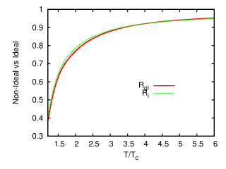
Figure 1: (Color online) $\eta$ relative to the that obtained using the ideal EOS for QGP, in the gluonic sector, and the (2+1)-flavor is plotted as a function of $T/T_{c}$. The solid curve denotes the gluonic sector and dashed line denotes the (2+1)-flavor. Both $R_{gi}$ and $R_{i}$ approach to the ideal limit asymptotically.

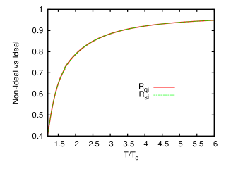
Figure 2: (Color online) $\eta$ relative to the that obtained using the ideal EOS for the QGP, in the matter sector. The $R_{qi}$ is $\eta$ relative to $\eta^{Id}$ in the light-quark sector, and similarly $R_{si}$ is for the strange quark sector. Both the curves sits on the top of each other since the mass effects from the strange-quark sector do not play significant role here.

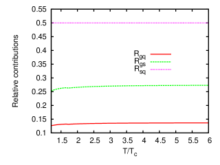
Figure 3: (Color online) Shear viscosity in effective gluonic sector relative to matter sector. The solid lines denotes $\eta_{g}$ relative to $\eta_{q}$, thin dashed lines (middle) represents $\eta_{g}$ relative to $\eta_{s}$, and upper thick dashed line represents $\eta_{s}$ relative to $\eta_{q}$, as a function of $T/T_{c}$.

The quantities defined in Eqs. (III.1-41) have been shown as a functions of $T/T_{c}$, in Figs. 1-4. The ratios $R_{gi}$ and $R_{i}$ are shown as a function of temperature in Fig. 1. The parameter $\hat{q}$ is assumed to be same in the interacting and ideal sector. We have considered temperature dependence beyond $1.2T_{c}$. Both $R_{gi}$, and $R_{i}$ show that interactions significantly modify the shear viscosity in the gluonic sector and the (2+1)-flavor QCD at lower temperatures. Both of them lie within the range $\{0.40,0.97\}$ for the temperature range, $\{T/T_{c}=1.2,6.0\}$. $R_{qi}$ and $R_{si}$ are shown in Fig. 2 as a function of temperature. Both of them sit on the top of each other. This is not surprising since the mass effects coming from the strange quark sector contribute negligibly in the temperature range considered here. The light quark sector and strange quarks differ with each other by a factor of two coming from the degrees of freedom. While considering the ratio $R_{si}$ it cancels from the numerator and denominator. From Fig.2, it is evident that the hot QCD interactions significantly modify the shear viscosity in the matter sector same as in the gluonic sector as compared to the ideal counter parts. All of them approaches asymptotically to the ideal limit which is nothing but unity. These observations suggest that $\eta$ could be thought of as a good diagnostic tool to distinguish various equations of state at the RHIC and the LHC.

Next, we investigate the gluonic shear and bulk viscosities relative to that of the matter sector. The relevant quantities in this context of $\eta$ are $R_{gq}$, $R_{gs}$, and $R_{sq}$ given in Eq.(40). These are shown as a function of temperature in Fig. 3. On the other hand for $\zeta$, $R^{qg}$, $R^{qs}$, and $R^{sq}$ are shown as a function of temperature in Fig. 4. It can be observed from Fig. 3, and Fig. 4 that the matter sector contributions significantly dominate over the gluonic contributions as far as the $\eta$ and $\zeta$ are concerned. This could perhaps be understood by the following facts, viz., the higher transport rates in the gluonic sector as compared to quark sector as encoded in $\hat{q}$, and the interactions entering through the effective fugacities $z_{g}$ and $z_{q}$. Quantitatively, $\eta_{g}$ is $\sim 0.125\eta_{q}$, and $0.250\eta_{s}$ at $T=1.20T_{c}$, and increases quite slowly as a function of $T/T_{c}$ reaching around $0.135\ \eta_{q}$ around $6T_{c}$ (see Fig. 3). The $\eta_{s}$ almost stays $0.5\ \eta_{q}$ for the considered range of temperature (contribution from the strange quark mass is almost negligible). From Fig. 4, it can be observed that $R^{gq}$ and $R^{gs}$ have same qualitative behavior as a function of temperature. The quantitative difference is because of a factor $\sim 2$, since $\zeta_{s}\sim 0.5\zeta_{q}$. Again the mass effects in the strange quark-sector play almost negligible role. The ratio $R^{gq}$ initially increases and attains a peak around $T/T_{c}\sim 1.37$ and then decreases sharply until $T/T_{c}=1.6$ and slightly increases beyond $1.6$ and indicating towards the saturation at higher temperatures. Quantitatively, $\zeta_{g}\approx 0.27\zeta_{q}$ around $1.2T_{c}$, and $0.13\zeta_{q}$ at $3.0T_{c}$. These observations are very crucial in deciding the temperature dependence of $\eta$ and $\zeta$, and the ratios $\eta/{\mathcal{S}}$, $\zeta/{\mathcal{S}}$ and $\zeta/\eta$. Most of the recent studies devoted to the $\eta$ and $\zeta$ draw inferences for the QGP which are purely based on the study of the pure $SU(3)$ sector of QCD only. The matter sector has largely been ignored. In the light of the above observations, it is not desirable to exclude the matter sector since the dominant contributions are from there. Finally, we can obtain the exact value of the ratios $\eta/{\mathcal{S}}$, and $\zeta/{\mathcal{S}}$ by employing the values of $\hat{q}$ quoted earlier ($\hat{q}=4.5GeV^{2}/fm$ for gluons and $2.0GeV^{2}/fm$ for quarks at $T=400MeV$). The ratio, $\eta/{\mathcal{S}}$ thus obtained as $0.570$ and $\zeta/{\mathcal{S}}$ came out to be $0.057$ at $T=400MeV$. As discussed earlier, to obtain the exact temperature dependence of $\eta$, and $\zeta$, one requires to fix the temperature dependence of $\hat{q}$ within the quasi-particle model employed here. This will be taken up separately in the near future. The quantity which can be determined unambiguity is the ratio $\zeta/\eta$ which is very crucial in deciding when the hot QCD becomes conformal. In other words, until what value of the temperature the effects coming from $\zeta$ are important while studying the QGP. We shall now proceed to discuss these issues next.

III.2 The ratio $\zeta/\eta$

The behavior of the ratio $\zeta/\eta$ as a function of temperature is shown in Fig. 5, and the temperature dependence of the ratios $\frac{\eta}{S}\equiv\frac{\eta\hat{q}}{T^{3}{\mathcal{S}}}$ and $\frac{\zeta}{{\mathcal{S}}}\equiv\frac{\zeta\hat{q}}{T^{3}{\mathcal{S}}}$, is shown in Fig. 6.

Most importantly, from Fig. 5, clear indications are observed that $\zeta$ in the gluonic sector, and the (2+1)-flavor QCD diverge as we approach closer to $T_{c}$ (the results are not shown around $T_{c}$, since such a quasi-particle picture may not be valid there.). The quantity $\zeta/\eta$ shows sharp decrease until one reaches up to $1.4T_{c}$ in the gluonic sector and $1.6T_{c}$ in the (2+1)-flavor QCD sector. Beyond that the decrease becomes slow and the ratio slowly approaches to zero. Such a behavior of $\zeta/\eta$ as a function of temperature could mainly be described in the formal expressions in Eqs. (II.4), and (II.4), and decided only by the temperature dependence of $c_{s}^{2}$ but also by the energy-dispersion relations, $\omega_{g,q,s}$, and the temperature dependence of the effective fugacities, $z_{g,q}$. It is evident that there is no way to obtain a $(c_{s}^{2}-\frac{1}{3})^{2}$ factor out from the expression while performing the integration. However, such a scaling could be realized whenever $p<<T^{2}\partial_{T}(ln(z_{g,q}))$, and $\omega_{g,q,s}$ happen to be independent of $z_{g}$ and $z_{q}$, and the thermal distribution of quai-partons show near ideal behavior. It may perhaps be realized at a very high temperature which are not relevant to study the QGP in the RHIC and the LHC. Therefore, $\zeta/\eta$ obtained here does not follow either a quadratic scaling or a linear scaling with the conformal measure $(c_{s}^{2}-\frac{1}{3})$. The same conclusions were obtained in the case of pure gauge theory recently chandra_bulk . Note that for the scalar field theories, $\zeta/\eta=15(c_{s}^{2}-\frac{1}{3})^{2}$ (quadratic scaling) scalar , and it has been found to be true for a photon gas coupled with the matter weinberg . The quadratic scaling is also valid in the case of perturbative QCD with a proportionality factor different from $15$ moore_1 . Furthermore, in the case of near conformal theories with gravity duals, $\zeta/\eta$ shows linear dependence on ($c_{s}^{2}-\frac{1}{3}$) confo .

Finally, in Fig. 6, $\frac{\eta}{S}$ and $\frac{\zeta}{S}$ are plotted as a function of $T/T_{c}$ (here the quantity $S$ is related to the entropy density (${\mathcal{S}}$) as $S=\frac{{\mathcal{S}}\hat{q}}{T^{3}}$. For the entropy density, we utilize the quasi-particle results which are shown to be consistent with the predictions of lattice QCD, and in all the plots $c_{s}^{2}$ has been obtained from the quasi-particle model employing the method quoted in gupta_cs . Interestingly, these are of same order at $T=1.2T_{c}$. Below that temperature the latter dominates over the former and vice versa for $T\geq 1.2T_{c}$. The former increases, in contrast to latter as a function of $T/T_{c}$. There is a sharp increase shown by the latter until one reaches $1.4T_{c}$, and beyond that the decrease is slower and one is quite close to the conformal limit of QCD. The important inference that could be drawn from here is that while studying the QGP one needs to incorporate the effects of both shear and bulk viscosities until approximately $1.5T_{c}$. This confirms our viewpoint that both $\eta$ and $\zeta$ have a significant impact on the properties of the QGP at the RHIC and the LHC.

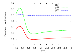
Figure 4: (Color online) Temperature dependence of relative quasi-parton bulk viscosities. The solid line shows the behavior of $\zeta_{g}$ relative to $\zeta_{q}$, thin dashed line shows the behavior of $\zeta_{g}$ relative to $\zeta_{s}$, and the thick dashed line shows the behavior of $\zeta_{s}$ relative to $\zeta_{q}$, as a function of $T/T_{c}$.

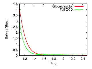
Figure 5: (Color online) Temperature dependence of the ratio $\zeta/\eta$, in the effective gluonic sector, and the (2+1)-flavor QCD. The solid line represents the gluonic sector, and the dashed line represents the (2+1)-flavor case.

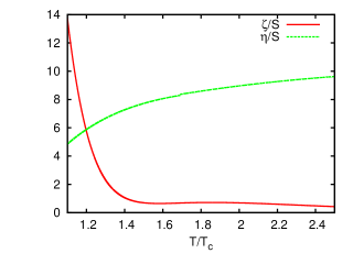
Figure 6: (Color online) The temperature dependence of the quantities, $\eta/S$ and $\zeta/S$ in the (2+1)-flavor QCD. Here $S=\frac{{\mathcal{S}}T^{3}}{\hat{q}}$, where ${\mathcal{S}}$ denotes the entropy density.

IV Conclusions and future prospects

In conclusion, the shear and bulk viscosities of the hot QCD are estimated by combining a semi-classical transport equation with a quasi-particle realization of the (2+1)-flavor lattice QCD. The effective gluonic sector contributes an order of magnitude lower as compared to the matter sector while determining the transport coefficients of the hot QCD and the QGP. This could perhaps be understood in terms of transport cross-sections of gluons and quark-antiquarks. Since transport coefficients are inversely proportional to the cross-sections. The bulk viscosity of the (2+1)-flavor QCD is found to be equally significant as the shear viscosity while modeling the QGP. Indications are seen regarding a blow up in the bulk viscosity as we go closer to $T_{c}$.

The temperature dependence of the ratio $\zeta/\eta$ suggests that the QGP becomes almost conformal around $1.4T_{c}-1.5T_{c}$. The ratio sharply decreases from $T=1.1T_{c}-1.4T_{c}$, and beyond that slowly approaches to zero. Therefore, in this regime we can ignore the effects of $\zeta$ while studying the hydrodynamic evolution and properties of the QGP. We further found that $\eta$ and $\zeta$ are of same order around $T=1.2T_{c}$. For temperatures lower than that $\zeta$ is dominant and for higher temperatures, $\eta$ is dominant. Importantly, both $\eta$ and $\zeta$ came out to be highly sensitive to the presence of interactions. This can be visualized from the modulation of $\eta$, as compared to its ideal counter part, and large and rising value of $\zeta$ for the temperatures that are closer to $T_{c}$ (due to large interaction measure there). The above conclusions are based on the fact that the ratio $\hat{q}_{g}/\hat{q}_{q}$ is temperature independent which is approximately true with the definition of $\hat{q}$ considered in the present analysis (leading order in perturbative QCD). A generalization of the definition of the $\hat{q}$ in view of the quasi-particle picture may induce both qualitative and quantitative modifications to the ratio $\zeta/\eta$, and will be investigated in the near future.

It would be a matter of immediate future investigation to utilize the more recent lattice data, and compare the predictions for the data from the hot QCD collaboration leos_lat , and the Wuppertal-Budapest collaboration leos1_lat . This would indeed be helpful in understating the impact of lattice artifacts, and uncertainties on the transport properties of the QGP.

The investigations on the other contributions to the shear and bulk viscosities (collisional etc.), and their interplay with the corresponding anomalous transport coefficients will be a matter of future investigations. It will be interesting to include the effects of non-vanishing baryon density to the transport coefficients of the QGP. Moreover, one could include the anomalous transport coefficients in the Boltzmann-transport theory approach and study the impact on the response functions and quarkonia physics along the lines of  chandra_nucla ; chandra_iitr , as well as dilepton production at the RHIC and the LHC. These ideas will be studied in the near future.

References

- (1) J. Adams et al. (STAR collaboration), Nucl. Phys. A757, 102 (2005); K. Adcox et al. (PHENIX Collaboration), ibid. A757, 184 (2005); Back et al. (PHOBOS Collaboration), ibid. A757, 28 (2005); A. Arsence et al. (BRAHMS Collaboration), ibid. A757, 1 (2005).
- (2) Y. Aoki et al., Nature 443, 675 (2006); F. Karsch, hep-lat/0601013; Journal of Physics: Conference Series 46, 121 (2006).
- (3) M. Luzum, P. Romatschke, Phys. Rev. C 78, 034915 (2008).
- (4) H. Song, U. W. Heinz, Nucl. Phys. A830, 467c (2009).
- (5) K. Paech, S. Pratt, Phys. Rev. C 74, 014901 (2006); S. Pratt, arXiv:1003.0413v3 [nucl-th].
- (6) J. R. Bhatt, H. Mishra, V. Srikanth, JHEP 1011, 106 (2010); arXiv:1101.5597 [hep-ph]; Phys. Lett. B704, 486 (2011).
- (7) E. M. Lifshitz and L. P. Pitaevskii, Physical Kinetics (Landau and Lifshitz), Vol. 10 (Pergamon Press, NewYork 1981).
- (8) M. S. Green, J. Chem. Phys. 22, 398 (1954); R. Kubo, J. Phys. Soc. Jpn. 12, 570 (1957).
- (9) G. Boyd et. al, Phys. Rev. Lett. 75, 4169 (1995); Nucl. Phys. B 469, 419 (1996); M. Panero, Phys. Rev. Lett. 103, 232001 (2009); F. Karsch, E. Laermann, A. Peikert, Phys. Lett. B 478, 447 (2000); M. Cheng et. al, Phys. Rev. D 77, 014511 (2008); A. Bazavov et. al, Phys. Rev. D 80, 014504 (2009); M. Cheng et. al, Phys. Rev. D 81,054504 (2010).
- (10) S. Borsanyi et. al, JHEP 1009,073 (2010); JHEP 11, 077 (2010); Y. Aoki et al., JHEP 0601, 089 (2006); JHEP 0906, 088 (2009).
- (11) H. B. Meyer, Phys. Rev. D 76, 10171 (2007); Lacey et. al, Phys. Rev. Lett. 98, 092301 (2007); Zhe Xu and C. Greiner, Phys. Rev. Lett. 100, 172301 (2008); Zhe Xu, C. Greiner, H. Stoecker, Phys. Rev. Lett. 101, 082302 (2008); Adare et. al, Phys. Rev. Lett. 98, 172301 (2007); S. Gavin and M. Abdel-Aziz, Phys. Rev. Lett. 97, 162302 (2006); A. Buchel, Phys. Lett. B 663, 286 (2008); P. Kovtun, D. T. Son, A. O. Starinets, Phys. Rev. Lett. 94, 111601 (2005).
- (12) M. Asakawa, S. A. Bass, B. Müller, Phys. Rev. Lett. 96, 252301 (2006); Prog. Theor. Phys. 116, 725 (2007).
- (13) V. Chandra and V. Ravishankar, Euro. Phys. J C 59, 705 (2009).
- (14) V. Chandra and V. Ravishankar, Euro. Phys. J C 64, 63 (2009).
- (15) F. Karsch, D. Kharzeev, K. Tuchin Phys.Lett. B 663, 217 (2008) ; D. Kharzeev, K. Tuchin, JHEP 09, 093 (2008).
- (16) H. B. Meyer, Phys. Rev. Lett. 100, 162001 (2008).
- (17) A. Buchel, Phys. Lett. B 663, 286 (2008).
- (18) V. Chandra, Phys. Rev. D 84, 094025 (2011).
- (19) M. Krzewicki (ALICE Collaboration), QM-2011, arXiv:1107.0080v1 [nucl-ex].
- (20) K. Aamodt et al. (The Alice Collaboration), arXiv:1011.3914 [nucl-ex]; Phys. Rev. Lett. 105, 252301 (2010); Phys. Rev. Lett. 106, 032301 (2011).
- (21) T. Hirano, P. Huovinen, Y. Nara, arXiv:1012.3955[nucl-th]; X. -F. Chen, T. Hirano, E. Wang, X. -N. Wang, H. Zhang, arXiv:1102.5614[nucl-th].
- (22) D. Teaney, Li Yan, arXiv:1010.1876 [nucl-th]; B. H. Alver, C. Gombeaud, M. Luzum, J.-Y. Ollitrault, Phys. Rev. C 82, 034913 (2010).
- (23) R. S. Bhalerao, M. Luzum, J.-Y. Ollitrault, arXiv:1106.4940[nucl-ex]; arXiv:1104.4740[nucl-th]; M. Luzum, J.-Y. Ollitrault, Phys. Rev. Lett. 106, 102301 (2011).
- (24) H. Song, U. W. Heinz, Phys. Rev. C 81, 024905 (2010).
- (25) G. S. Denicol, T. Kodama, T. Koide, Ph. Mota, Phys. Rev. C 80, 064901 (2009).
- (26) G. S. Denicol, T. Kodama, T. Koide, Ph. Mota, Nucl. Phys. A830, 729c (2009).
- (27) A. Monnai, T. Hirano, Nucl. Phys. A830, 471c (2009; Phys. Rev. C 80, 054906 (2009).
- (28) K. Rajagopal, N. Tripuraneni, JHEP 1003, 018 (2010); J. R. Bhatt, H. Mishra, V. Sreekanth arXiv:1103.4333.
- (29) M. J. Efaaf, Z.-Q. Su, W.-N. Zhang, arXiv:1008.1531.
- (30) D. Fernandez-Fraile, A. G. Nicola, Phys. Rev. Lett. 102, 121601 (2009).
- (31) R. J. Fries, B. Müller, Andreas Schäfer, Phys. Rev. C 78, 034913 (2008).
- (32) G. Torrieri, B. Tomasik, I. Mishustin Phys. Rev. C 77, 034903 (2008); Acta. Phys. Polon. B 39, 1733 (2008).
- (33) P. Bozek, Phys. Rev. C 81, 034909 (2010).
- (34) G. D. Moore, O. Saremi, JHEP 0809, 015 (2008).
- (35) K. Rajgopal, N. Tripuraneni, JHEP 1003, 018 (2010).
- (36) J. R. Bhatt, H. Mishra, V. Srikanth, arXiv:1101.5597 [hep-ph].
- (37) A. Klimek, L. Leblond, A. Sinha, Phys. Lett. B701, 144 (2011), arXiv:1103.3987[hep-th] .
- (38) R. C. Myers, M. F. Paulos, A. Sinha, JHEP 0906, 006 (2009), Phys. Rev. D 79, 041901; A. Buchel, R. C. Myres, A. Sinha, JHEP 0903, 084 (2009).
- (39) H. B. Meyer, Phys. Rev. Lett. 100, 162001 (2008).
- (40) D. Teaney, Phys. Rev. D 74, 0450125 (2006) (hep-ph/0602044); G. D. Moore, O. Saremi, JHEP 0809, 015 (2008) (arXiv:0805.4201[hep-ph]); P. Romatschke, D. T. Son, Phys. Rev. D 80, 065021 (2009) (arXiv:0903.3946).
- (41) H. B. Mayer, JHEP 1004, 099 (2010) (arXiv:1002.3343[hep-lat]).
- (42) A. Nakamura, S. Sakai, Phys. Rev. Lett. 94, 072305 (2005); Nucl. Phys. A 774, 775 (2006).
- (43) S. Gupta et. al, Science 332, 1525 (2011), arXiv:1105.3934 [hep-ph].
- (44) V. Chandra, R. Kumar, V. Ravishankar, Phys. Rev. C 76, 054909 (2007); Indian J. Phys. 84, 1789 (2010).
- (45) V. Chandra, A. Ranjan, V. Ravishankar, Euro. Phys. J. A 40, 109 (2009); arXiv:0801.1286[hep-ph].
- (46) V. Chandra, V. Ravishankar, Phys. Rev. D 84, 074013 (2011).
- (47) P. Chakraborty, J. I. Kapusta, Phys. Rev. C 83, 014906 (2011), arXiv:1006.0257.
- (48) C. Sasaki, K. Redlich, Phys. Rev. C 79, 055207 (2009).
- (49) S. Mrowczynski, Phys. Rev. C 49, 2191 (1994); M. Strickland, Braz. J. Phys. 37, 762 (2007); hep-ph/0611349; P. Arnold, G. D. Moore, Phys. Rev. D 73, 025013 (2006).
- (50) M. Asakawa, S. A. Bass, B. Müller, Phys. Rev. Lett. 96, 252301 (2006); J. Phys. G 34, S839 (2007).
- (51) A. Majumdar, B. Müller, X. -N. Wang, Phys. Rev. Lett. 99, 192301 (2007).
- (52) T. H. Dupree, Phys. Fluids 9, 1773 (1966); ibid. 11 2680 (1968).
- (53) T. Abe, K. Niu, J. Phys. Soc. Japan 49 717 (1980); ibid. 49 725, (1980).
- (54) E. S. Weibel, Phys. Rev. Lett. 2, 83 (1959).
- (55) S. Mr̀owczỳnski, Phys. Lett. B 214, 587 (1988); ibid. B 314, 118 (1993); P. Romatschke, M. Strickland, Phys. Rev. D 68 036004, (2003).
- (56) A. Peshier et. al, Phys. Lett. B 337, 235 (1994); Phys. Rev. D 54, 2399 (1996).
- (57) A. Peshier, B. Kämpfer, G. Soff, Phys. Rev. C 61, 045203 (2000); Phys. Rev. D 66, 094003 (2002); V. M. Bannur, Phys. Rev. C 75, 044905 (2007); ibid. C 78, 045206 (2008); JHEP 0709, 046 (2007); A. Rebhan, P. Romatschke, Phys. Rev. D 68, 0250022 (2003); M. A. Thaler, R. A. Scheider, W. Weise, Phys. Rev. C 69, 035210 (2004); K. K. Szabò, A. I. Tòth, JHEP 06, 008 (2003).
- (58) M. D’Elia, A. Di Giacomo, E. Meggiolaro, Phys. Lett. B 408, 315 (1997); Phys. Rev. D 67, 114504 (2003); P. Castorina, M. Mannarelli, Phys. Rev. C75, 054901 (2007); Phys. Lett. B 664, 336 (2007).
- (59) A. Dumitru, R. D. Pisarski, Phys. Lett. B 525, 95 (2002); K. Fukushima, Phys. Lett. B 591, 277 (2004); S. K. Ghosh et. al, Phys. Rev. D 73, 114007 (2006); H. Abuki, K. Fukushima, Phys. Lett. B 676, 57 (2006); H. M. Tsai, B. Müller, J. Phys. G 36, 075101 (2009).
- (60) J. -W. Chen, J. Deng, H. Dong, Q. Wang, arXiv:1107.0522v2[hep-ph].
- (61) J. -W. Chen, J. Deng, H. Dong, Q. Wang, Phys. Rev. D 83, 034031 (2011); ibid. D 84, 0399902(E) (2011).
- (62) P. Arnold, C. Dolan, G. D. Moore, Phys. Rev. D 74, 085021 (2006).
- (63) M. Bluhm, B. Kämpfer, K. Redlich, arXiv:1011.5634(nucl-th); arXiv:1101.3072[nucl-th]; A. S. Khvorostukhin, V. D. Toneev, D. N. Voskresersky, Phys. Rev. C 83, 035204 (2011); S. K. Das, Jan-e Alam, Phys. Rev. D 83, 114011 (2011); S. Plumari, W. M. Alberico, V. Greco, C. Ratti, Phys. Rev. D 84, 094004 (2011).
- (64) H. Zhang, J. F. Owens, E. Wang, X. -N. Wang, Phys. Rev. Lett. 98, 212301 (2007); A. Majumder, C. Nonaka, S. A. Bass, Phys. Rev. C 76, 041902 (2007); R. Bair et, al., Nucl. Phys. B 483, 291 (1997); N. Armesto, L. Cunqueiro, C. A. Salgado, W.-C. Xiang, JHEP 0802, 048 (2008).
- (65) X. N. Wang, X. F. Guo, Nucl. Phys. A696, 788 (2001); A. Majumdar, arXiv:0901.4516v2[nucl-th]; Phys. Rev. D 75, 014023 (2012).
- (66) P. Arnold, W. Xiao, Phys. Rev. D 78, 125008 (2008).
- (67) R. Horsley, W. Schoenmaker, Nucl. Phys. B280, 716 (1987).
- (68) S. Weinberg, Astrophys. J 168, 175 (1971).
- (69) P. Arnold, C. Dogan , Phys. Rev. D 74, 085021 (2006).
- (70) P. Benincasa, A. Buchal, A. O. Strarinets, Nucl. Phys. B733, 160 (2006); A. Buchal, Phys. Rev. D 72, 106002 (2005).
- (71) R. V. Gavai, S. Gupta, S. Mukherjee, PoS LAT 2005, 173 (2005).
- (72) M. Cheng et. al, Phys. Rev. D 77, (2008).
- (73) Special thanks to S. Datta for computing the contribution to the lattice EOS from the gluonic action with the same lattice set up of cheng .
- (74) K. Dusling, T. Schäfer, Phys. Rev. C 85, 044909 (2012).
- (75) K. Dusling, D. Teaney, Phys. Rev. C 77, 034905 (2008).
- (76) V. Chandra, V. Ravishankar, Nucl. Phys. A848, 330 (2010).
- (77) V. Agotiya, V. Chandra, B. K. Patra, Phys. Rev. C 80, 025210 (2009); Euro. Phys. J C 67, 465 (2010).