Doublon dynamics in the extended Fermi Hubbard model

Abstract

Two fermions occupying the same site of a lattice model with strongly repulsive Hubbard-type interaction $U$ form a doublon, a long-living excitation the decay of which is suppressed because of energy conservation. By means of an exact-diagonalization approach based on the Krylov-space technique, we study the dynamics of a single doublon, of two doublons, and of a doublon in the presence of two additional fermions prepared locally in the initial state of the extended Hubbard model. The time dependence of the expectation value of the double occupancy at the different sites of a large one-dimensional lattice is analyzed by perturbative arguments. In this way the spatiotemporal evolution of the doublon can be understood. The initial decay takes place on a short time scale $1/U$, and the long-time average of the decayed fraction of the total double occupancy scales as $1/U^{2}$. We demonstrate how the dynamics of a doublon in the initial state is related to the spectrum of two-fermion excitations obtained from linear-response theory, we work out the difference between doublons composed of fermions vs doublons composed of bosons, and we show that despite the increase of phase space for inelastic decay processes, the stability of a doublon is enhanced by the presence of additional fermions on an intermediate time scale.

I Introduction

Since the seminal work of Jaksch et al.,jaksch1998cold ultracold atomic gases in optical lattices have served as a valuable testing ground for the rich phenomenology of many-body models which originally were introduced in the context of condensed-matter physics.bloch2008manybodyultracoldgases ; trefzger2011ultracolddipgasesoptlatt ; lewenstein2007ultracoldatomicgases A nice example is the concept of repulsively bound pairs of fermions which can be studied in the strong-coupling regime of the Hubbard model or, as shown recently,wall2011quantuminterferencechargeexpaths in an organic salt at room temperature by means of ultrafast optical spectroscopy. Repulsively bound pairs, named doublons, are already known since the early work of Hubbardhubbard1963electron and were lately addressed in both theoretical and experimental work in bosonicwinkler2006repulsivelybound ; petrosyan2007quantumliquid ; petrosyan2008twopartstateshubbardmodel ; valiente2008quantumdynonetwobosonic ; valiente2009twopartboundstateexthubbard ; javanainen2010dimertwobosons1doptlatt as well as fermionicjochim2003becmolecules ; greiner2003emergencemolecularbecfermigas ; rosch2008metastable ; hassanieh2008excitonsin1dhubbard ; heidrichmeisner2009quantdistillation ; strohmaier2010observationdoublondecay ; hansen2011splithubbardbands ; enss2011lightconerenorm ; kajala2011xepdyn1dfermihubbardmodel Hubbard-type models. The fermionic case directly refers to condensed-matter systems, such as strongly correlated electrons in a valence band of transition-metals and their compounds, and two-particle electron spectroscopy.

A doublon is a pair of two fermions tightly bound to each other. The pair is itinerant, it propagates through the lattice and thereby acquires a certain energy dispersion. The pair may decay into its constituents. However, for strongly repulsive interaction $U>0$, this decay is suppressed very efficiently. The stability of the doublon appears as counterintuitive since an energy of the order of $U>0$ would be gained if the two fermions were propagating through the lattice independently. There is, however, a “repulsive binding” originating from energy conservation: For $U$ much larger than the nearest-neighbor hopping $J$, the excess energy $U$ cannot be accommodated in the kinetic energy of the two independent fermions which at most amounts to twice the bare bandwidth $W\propto J$.

In the strong-coupling limit, doubly occupied sites are created in different types of electron spectroscopies:potth2001theor The spectral function $A_{ij}(\omega)$ at positive frequencies $\omega>0$, obtained from the imaginary part of the one-particle Green’s function $\langle\negthinspace\langle\hat{c}^{\phantom{\dagger}}_{i\sigma};\hat{c}^{\dagger}_{j\sigma}\rangle\negthinspace\rangle$, is related to inverse photoemission, and the upper Hubbard band in the spectral function describes a final state with doubly occupied sites. The lower Hubbard band represents the analog of the upper Hubbard band in case of photoemission. For the Hubbard model on a bipartite lattice at half filling, it is obtained from the upper one by a particle-hole transformation and thus describes repulsively bound holes. Doublons can also be created in an otherwise empty valence band in a two-particle process, such as appearance-potential spectroscopy (APS), i.e., the “time inverse” of Auger-electron spectroscopy (AES). Here, two additional electrons (holes) are created, preferably at the same site, in the final state of APS (AES). Doublon bound states in APS/AES show up in the local two-particle Green’s function $\langle\negthinspace\langle\hat{c}^{\phantom{\dagger}}_{i\sigma}\hat{c}^{\phantom{\dagger}}_{i\bar{\sigma}};\hat{c}^{\dagger}_{i\sigma}\hat{c}^{\dagger}_{i\bar{\sigma}}\rangle\negthinspace\rangle$ as is well known from Cini-Sawatzky theory.cini1977two ; sawatzky1977quasiatomic ; nolting1990influence ; potth2001theor Furthermore, doublons appear in particle-hole excitations associated with Green’s functions of the type $\langle\negthinspace\langle\hat{c}^{\dagger}_{i\sigma}\hat{c}^{\phantom{\dagger}}_{j\sigma};\hat{c}^{\dagger}_{k\sigma}\hat{c}^{\phantom{\dagger}}_{l\sigma}\rangle\negthinspace\rangle$. In all mentioned cases, a doublon would be identified with a long-lived excitation at energies of the order of $U$.

Since a pair of fermions has bosonic character, the exciting question arises whether a macroscopically large number of doublons could Bose condensate at sufficiently low temperatures and high densities. This has been studied theoretically for doublons of bosonic petrosyan2007quantumliquid and of fermionic constituents.rosch2008metastable The two main questions in this context concern the doublon stability and the effective interaction between doublons: First, a sufficiently long lifetime of doublons is required for a possible Bose condensation taking place in a metastable state. Recent experiments with fermionic atoms in optical lattices strohmaier2010observationdoublondecay in fact give a lifetime which increases exponentially with $U$. Second, the physical interactions between the constituents give rise to an effective doublon-doublon interaction in an effective low-energy theory. A strong repulsive $U$, for example, leads to an effectively attractive interaction between doublons formed by two bosons. It has been shown that this inhibits condensation but rather favors phase separation.petrosyan2007quantumliquid

The real-time dynamics of a spatially extended system of strongly correlated fermions poses a notoriously complex many-body problem which is hardly accessible to exact analytical or numerical methods. Either one has to tolerate mean-field-type approximations like in the nonequilibrium dynamical mean-field approach schmidt2002noneqDMFTstrongcorrsys ; freericks2006noneqDMFT ; eckstein2009thermalization or has to restrict oneself to one-dimensional or impurity-type systems to render an application of time-dependent renormalization-group approaches cazalilla2002tDMRGsystmethodquantummanybodooeq ; white2004realtimevDMRG ; anders2005realtimedynquantimpsys-tDMRG possible. With the present paper we study a simplified problem with a drastically reduced Hilbert space dimension and focus on two and four spinful fermions with on-site ($U$) and nearest-neighbor interaction ($V$) on large one-dimensional lattices only. The time evolution of this few-fermion quantum system is accessible by a numerically exact Krylov-space approach.lanczos1950iteration ; park1986unitary ; saad1992analysiskrylovsubspaceapprox ; hochbruck1997krylov ; hochbruck1999exponentialintegrators ; molervanloan2003expmatrix ; manmana2005timev1d Our study tries to shed some light on the following issues discussed extensively in the recent literature:

For a single doublon prepared at a definite site initially, we show how the resulting propagation pattern is affected by $U$ and $V$ and how this is understood in terms of perturbative arguments in the strong-coupling limit. The manifestation of “energy conservation” will be analyzed by studying the short-time dynamics of a doublon.

The real-time dynamics of a quantum system in a highly excited state on the one hand and the spectrum of excitations out of thermal equilibrium, as obtained in linear-response theory, on the other hand are usually two completely different issues. Here, we discuss a one-to-one relation that is obtained for the case of a single doublon and therewith address the physics of the long-time stability of a single doublon.

The real-time dynamics of two doublons in different initial states is discussed. Particularly, the $V$ dependencies are interesting as there is a reduced effective doublon-doublon attraction in the Fermi opposed to the Bose case which is important to understand the competition between Bose condensation and phase separation of doublons.petrosyan2007quantumliquid ; rosch2008metastable

For a thermodynamically relevant number of fermions, one generally expects that with the presence of many additional degrees of freedom there is an enhanced probability for doublon decay since the doublon energy can be accommodated among different particles in a high-order scattering event. This is already seen by means of the ladder approximation applicable to the low-density limit where a strong initial decay at short times is observed followed by a slow exponential decay at long times.hansen2011splithubbardbands Here, this question is studied for the case of four fermions and discussed in the context of recent time-dependent density-matrix renormalization-group studies.hassanieh2008excitonsin1dhubbard ; enss2011lightconerenorm

The paper is organized as follows: The next section, Sec. II, introduces the model, the central observables and the Krylov approach. We start with the analysis of single-doublon propagation in Sec. III, discuss the effects of the nearest-neighbor interaction in Sec. IV and the short-time decay in Sec. V. The relation to APS is worked out in Sec. VI, and the long-time stability is discussed in Sec. VII. The second part of the paper is devoted to our four-fermion results: We discuss the dynamics of two doublons in Sec. VIII and doublon-fermion scattering in Sec. IX. Final remarks and conclusions are given in Sec. X.

II Extended Hubbard model and basic theory

Ultracold atoms, loaded into an optical lattice, are subject to different kinds of interaction. bloch2008manybodyultracoldgases ; trefzger2011ultracolddipgasesoptlatt ; lewenstein2007ultracoldatomicgases In the simplest cases these are short-ranged, like van der Waals forces, scaling as $1/r^{6}$ and hence approximately act on-site only. Depending on the atomic species, however, more general interactions can occur. For example, polarized dipolar atoms experience a dipole-dipole interaction given by $U_{\text{dd}}\propto(1-3\cos^{2}\theta)/r^{3}$. Depending on the angle $\theta$ between the dipole moments and their relative displacement vector, this can either be repulsive or attractive. It is comparatively long-ranged and usually modeled as an interaction between nearest neighbors. Overall, this motivates the extended Hubbard model:

$$\mathcal{H}=-J\sum_{\left<ij\right>}\sum_{\sigma}\hat{c}^{\dagger}_{i\sigma}\hat{c}^{\phantom{\dagger}}_{j\sigma}+U\sum_{i}\hat{n}^{c}_{i\downarrow}\hat{n}^{c}_{i\uparrow}\\ +\frac{V}{2}\sum_{\left<ij\right>}\sum_{\sigma\sigma^{\prime}}\hat{n}^{c}_{i\sigma}\hat{n}^{c}_{j\sigma^{\prime}}=:\mathcal{H}_{J}+\mathcal{H}_{U}+\mathcal{H}_{V}\,,$$ (1)

which also applies as a model description to electrons interacting via the screened Coulomb repulsion in condensed-matter systems, e.g. transition-metal compounds, if orbital degrees of freedom can be neglected. Here, $i$ and $j$ refer to the sites of a one- or higher-dimensional lattice, $\left<ij\right>$ denotes nearest neighbors, and $\sigma=\uparrow,\downarrow$ is the spin projection. $J$ is the nearest-neighbor hopping, and $U$ and $V$ the on-site and the nearest-neighbor interaction strength.

Our central object of interest is the time-dependent expectation value of both the local and the total double occupancy, namely $\left<\mathcal{D}_{i}(t)\right>$ and $\left<\mathcal{D}(t)\right>=\sum_{i}\left<\mathcal{D}_{i}(t)\right>$, respectively. Here, the local double-occupation operator is given by $\mathcal{D}_{i}=\hat{n}^{c}_{i\uparrow}\hat{n}^{c}_{i\downarrow}$ where $\hat{n}^{c}_{i\sigma}=\hat{c}^{\dagger}_{i\sigma}\hat{c}^{\phantom{\dagger}}_{i\sigma}$ is the number operator and where $c^{(\dagger)}_{i\sigma}$ denotes the annihilation (creation) operator for a fermion at site $i$ with spin $\sigma$. The time dependence of the expectation value is due to the time dependence of the system’s state $\left|\psi(t)\right>=\exp(-i\mathcal{H}t)\left|\psi_{\text{ini}}\right>$ where $\left|\psi_{\text{ini}}\right>$ is the state in which the system was prepared initially at time $t=0$.

For systems with moderately large Hilbert-space dimensions $d$, the numerically exact time evolution of a given initial state is accessible by means of a time-dependent Krylov-space technique. lanczos1950iteration ; park1986unitary ; saad1992analysiskrylovsubspaceapprox ; hochbruck1997krylov ; hochbruck1999exponentialintegrators ; molervanloan2003expmatrix ; manmana2005timev1d Some details of the method are summarized in Appendix A.

In the following we concentrate on a one-dimensional lattice with $L$ sites and two or four fermions with equal number of up and down spins. Thereby different processes, such as the propagation and decay of a single doublon as well as doublon-fermion and doublon-doublon scattering, can be studied. For two fermions, the Hilbert-space dimension is $d=L^{2}$ and we opt for a lattice with $L=100$ sites. For four fermions, it is $d=L^{2}(L-1)^{2}/4$ and we shorten the lattice to $50$ sites. In either case, periodic boundary conditions are assumed.

III Propagation of a single doublon

To begin with, we consider the two-fermion system and assume that initially, at time $t=0$, both fermions are at the same site $i_{0}$, i.e. $|\psi_{\text{ini}}\rangle=\hat{c}^{\dagger}_{i_{0}\uparrow}\hat{c}^{\dagger}_{i_{0}\downarrow}\left|0\right>$. Figure 1 (left part) shows the time evolution of the expectation value of the local double occupancy at $V=0$ and for strong on-site interaction $U=8J$. The nearest-neighbor hopping $J=1$ fixes the energy and time scales. We notice different effects. First of all, the doublon delocalizes. The double occupancy $\left<\mathcal{D}_{i}(t)\right>$ at the site where the doublon has been prepared initially ($i_{0}=50$) quickly decreases, and in the course of time $\left<\mathcal{D}_{i}(t)\right>$ basically spreads out over the entire lattice. For the time scale $t<100$ shown in the figure, the “light cones” do not yet interfere through the periodic boundary. Second, there is doublon decay. The top panel of Fig. 1 shows the total double occupancy $\left<\mathcal{D}(t)\right>=\sum_{i}\left<\mathcal{D}_{i}(t)\right>$. There is a significant decay from the initial value $\left<\mathcal{D}(t)\right>=1$ to about $\left<\mathcal{D}(t)\right>\approx 0.9$ in a very short time $t\lesssim 0.5$ (not resolved on the scale of the figure), followed by an almost constant trend. The tiny fluctuations around the constant “final” value are simply reflecting the fact that the total double occupancy does not commute with the Hamiltonian.

Except for the decay of the doublon, all the details of the entire propagation profile are fully captured by a simple analytical description in an effective low-energy model; see the right panel of Fig. 1. As described in Appendix B, this effective model is obtained by a unitary transformation to project out the energetically well separated high-energy part of the spectrum, thereby generating effective low-energy couplings perturbatively, in powers of $J/U$: foldy1950diractheory ; chao1977degperturbationtheory ; chao1977kineticexchange ; spalek2007tJmodel ; fazekas1999lecturenoteselectroncorr

$$\mathcal{H}_{\text{eff}}^{(d)}=\frac{J^{\prime}}{2}\sum_{\left<ij\right>}\hat{d}^{\dagger}_{i}\hat{d}^{\phantom{\dagger}}_{j}+(J^{\prime}+U)\sum_{i}\hat{n}^{d}_{i}-\frac{J^{\prime}}{2}\sum_{\left<ij\right>}\hat{n}^{d}_{i}\hat{n}^{d}_{j}\,.$$ (2)

Here, $\hat{d}^{\dagger}_{i}=\hat{c}^{\dagger}_{i\uparrow}\hat{c}^{\dagger}_{i\downarrow}$ and $\hat{d}^{\phantom{\dagger}}_{i}$ describe hard-core bosons with the constraint $\hat{d}^{\dagger}_{i}{}^{2}=0$. Furthermore, $\hat{n}^{d}_{i}=\hat{d}^{\dagger}_{i}\hat{d}^{\phantom{\dagger}}_{i}=\hat{n}^{c}_{i\uparrow}\hat{n}^{c}_{i\downarrow}$ is the local doublon number. Hence Eq. (2) involves doublon degrees of freedom only and takes the form of an extended Bose-Hubbard model with the effective hopping $J^{\prime}=4J^{2}/U$ and an (in case of positive $U$) attractive nearest-neighbor interaction.

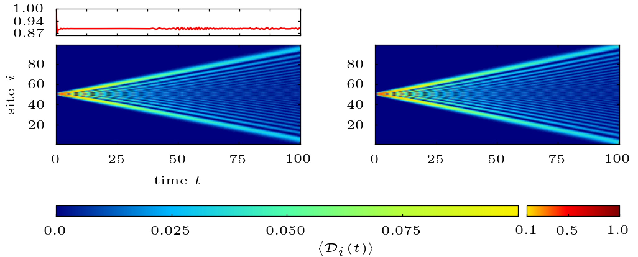
Figure 1: Temporal evolution of the expectation value (see color code) of the double occupancy at sites $i=1,...,L$. Left: Numerical results for the one-dimensional Hubbard model ($V=0$) with $L=100$ sites and periodic boundary conditions at $U=8J$. Initially, at $t=0$, the two-fermion state has been prepared as a doublon at $i_{0}=50$. Top: Time evolution of the expectation value of the total double occupancy. Right: Corresponding analytical results of the effective model, see Eq. (3). Note that most of the color range is used to display expectation values less than $0.1$, as shown in the color bar below. The time $t$ is measured in units of the inverse hopping $1/J$.

(a) $U=0,V=-10$

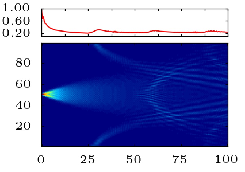
(b) $U=0,V=-5$

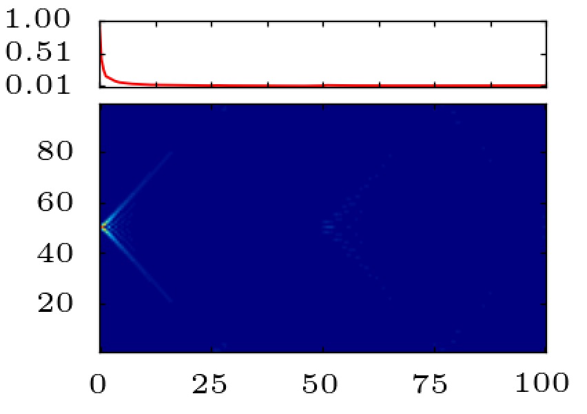
(c) $U=0,V=0$

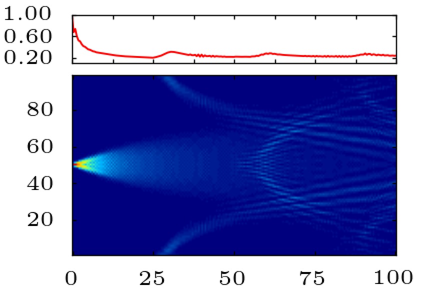
(d) $U=0,V=5$

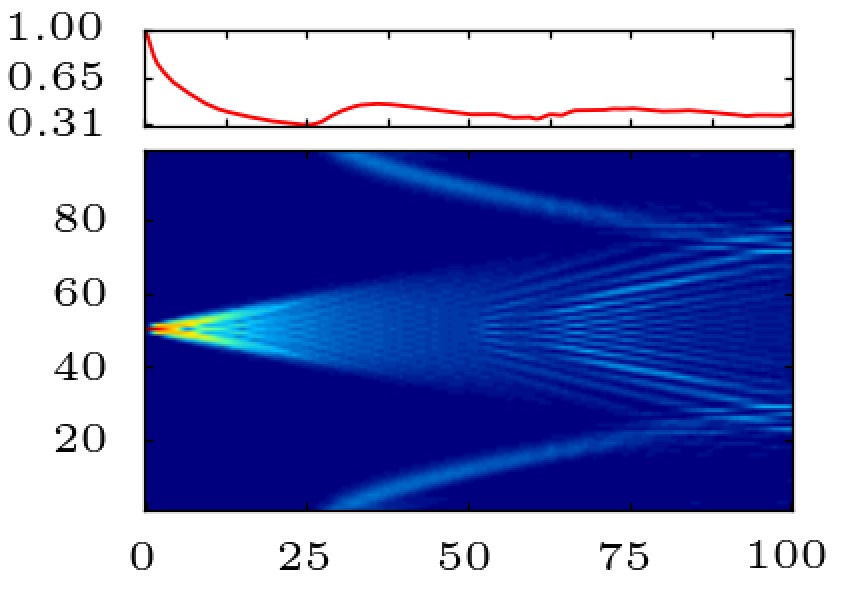
(e) $U=0,V=10$

(f) $U=5,V=-10$

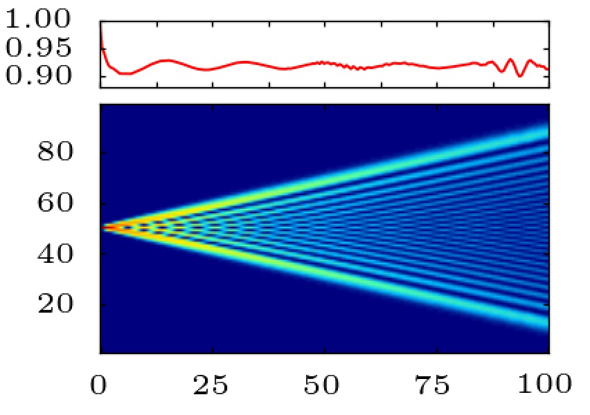
(g) $U=5,V=-5$

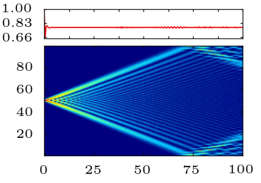
(h) $U=5,V=0$

(i) $U=5,V=5$

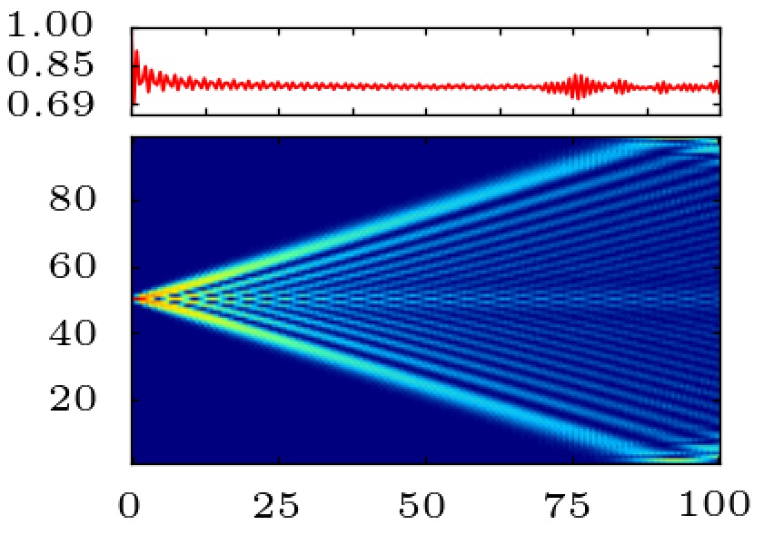
(j) $U=5,V=10$

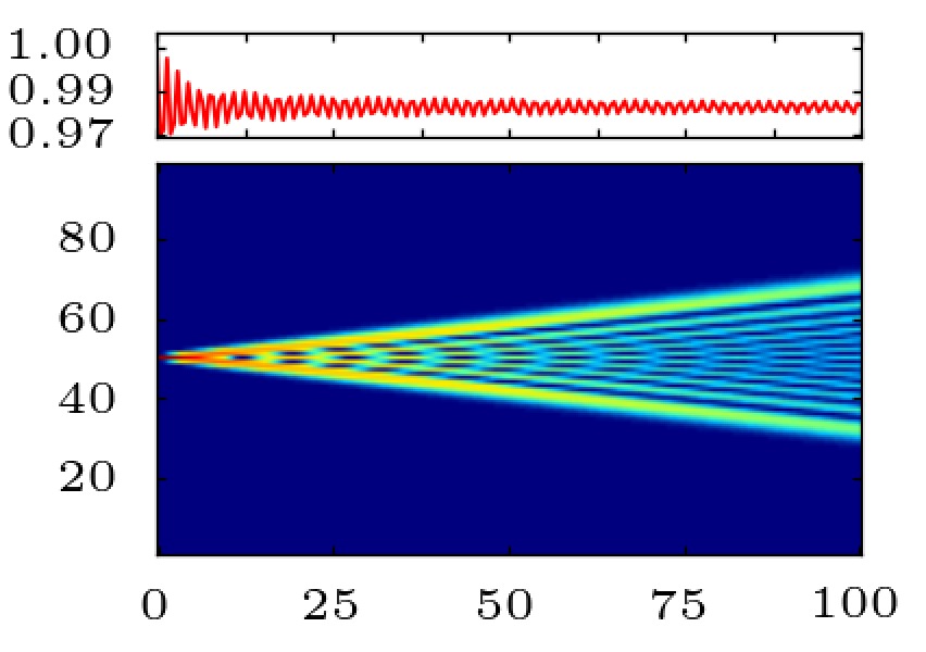
(k) $U=10,V=-10$

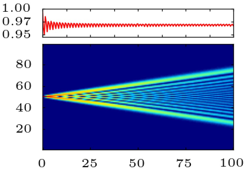
(l) $U=10,V=-5$

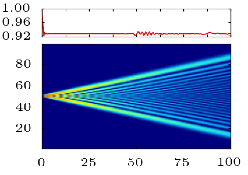
(m) $U=10,V=0$

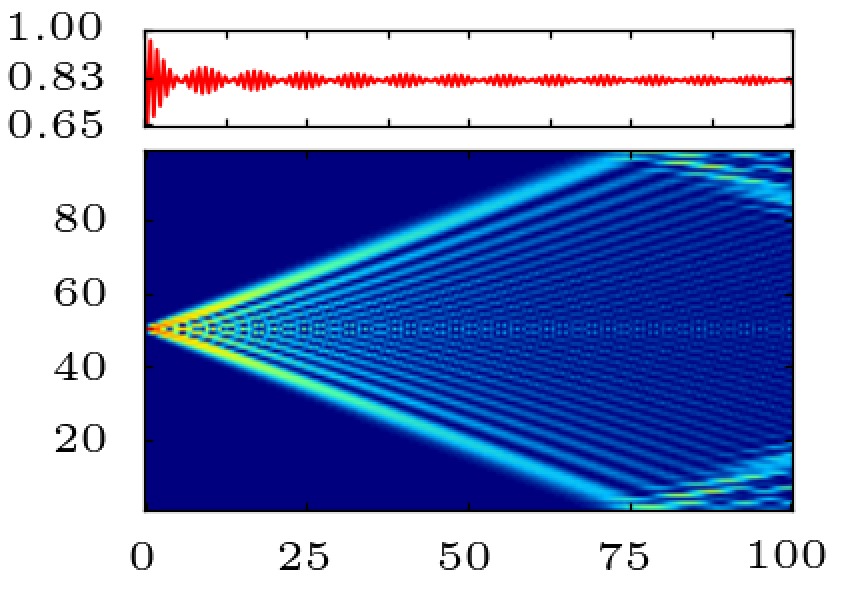
(n) $U=10,V=5$

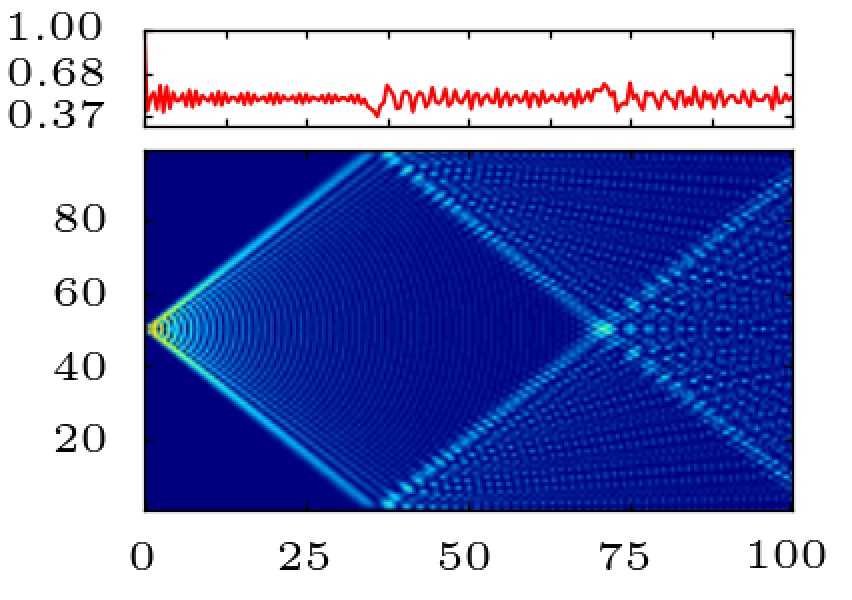
(o) $U=10,V=10$

Figure 2: Time-dependent expectation value of the local (main panels) and total double occupancy (small top panels) for two fermions initially prepared at the same site $i_{0}$ of a one-dimensional lattice with $L=100$ sites and periodic boundary conditions. Results for on-site interaction $U=0,5,10$ and nearest-neighbor coupling $V=0,\pm 5,\pm 10$, as indicated. Note that for the total double occupancy the scale of the $y$-axis differs from case to case. The color code is the same as in Fig. 1 and the same for all plots.

For a system with a single doublon only, the interaction term can be disregarded, and the resulting free tight-binding Hamiltonian is diagonalized by Fourier transformation. In the limit $L\rightarrow\infty$, the time-dependent local double occupancy in the effective model is then found to be given by the $k$th Bessel function of the first kind $\mathcal{J}_{k}$,

$$\left<\mathcal{D}_{i}^{\text{eff}}(t)\right>=\mathcal{J}_{i-i_{0}}^{2}(J^{\prime}t)\,,$$ (3)

if the doublon was prepared at site $i_{0}$ initially. Note that the total double occupancy is conserved, since $\sum_{k=-\infty}^{\infty}\mathcal{J}_{k}^{2}(x)=1$ for all $x$.

The time dependence of the expectation value of the local double occupancy, as given by Eq. (3), is shown in Fig. 1 (right). While effects due to doublon decay are neglected at this level, doublon-propagation effects should be captured qualitatively correct. Comparing with the exact numerical result (Fig. 1, left), we note that the effective model provides an excellent description of the propagation already for $U=8J$.

The effect of varying $U$ can be seen in Fig. 2. The panels Fig. LABEL:sub@fig:oneU0V0, LABEL:sub@fig:oneU5V0, and LABEL:sub@fig:oneU10V0 give the result of the full model for $U=0$, $U=5J$ and $U=10J$. We note that the mobility of the doublon decreases with increasing $U$ which, in the effective model, is due to the reduced doublon hopping $\sim 1/U$. The interference pattern visible for $U=5J$ in panel Fig. LABEL:sub@fig:oneU5V0 is due to the finite system size and periodic boundary conditions. Apart from that, however, the pattern does not change much qualitatively as compared to $U=10J$. This is worth mentioning since $U=5J$ is well below the critical $U$ (of the order of twice the free bandwidth $2W=8J$) at which the two-particle excitation spectrum, related to the APS Green’s function $\langle\negthinspace\langle\hat{c}^{\phantom{\dagger}}_{i\sigma}\hat{c}^{\phantom{\dagger}}_{i\bar{\sigma}};\hat{c}^{\dagger}_{i\sigma}\hat{c}^{\dagger}_{i\bar{\sigma}}\rangle\negthinspace\rangle$, does change qualitatively since the correlation satellite splits off (see Ref. nolting1990influence, , for example). This reminds us that there is a clear conceptual difference between the two-particle spectrum that refers to excitations starting from the system’s ground state on the one hand and the temporal evolution of a highly excited initial state on the other.

IV Effects of nearest-neighbor interaction

The remaining panels of Fig. 2 show propagations patterns for finite nearest-neighbor interaction $V$. For $U=10J$, see last row in Fig. 2, we find a decreasing mobility of the doublon with increasing difference between the on-site and the nearest-neighbor interaction strengths $U-V$. Similar to the discussion in the preceding section, this trend is easily explained in an effective model that preserves the total double occupancy. This can be derived, for example, by standard second-order perturbation theory around the $J=0$ limit and yields an effective doublon hopping amplitude

$$J^{\prime}=4\frac{J^{2}}{U-V}\,.$$ (4)

This corresponds to a sequence of two virtual hopping processes: In the first, one of the two fermions composing the doublon hops to a nearest-neighbor site. Thereby, for $U>V$ ($U<V$), the energy $U-V$ is gained (has to be paid). The second nearest-neighbor hopping process leads to the recombination of the doublon, either at the same or at one of the adjacent sites.

Looking at the cone angle of the “light cone” in the propagation patterns in the last row and comparing the results with $U-V=20$ to $U-V=5$, the effective description yields the correct trend: As the expectation value of the double occupancy in the effective model depends on the product of $J^{\prime}$ and $t$ only, see Eq. (3), the time axis scales linearly with $J^{\prime}$. The effective doublon hopping also explains that the patterns in panels Figs. LABEL:sub@fig:oneU5V-10 and LABEL:sub@fig:oneU10V-5 and the patterns in Figs. LABEL:sub@fig:oneU5V-5 and LABEL:sub@fig:oneU10V0 as well as Figs. LABEL:sub@fig:oneU5V0 and LABEL:sub@fig:oneU10V5 are almost equal as $U-V$ is constant, respectively.

For $U=5J$, see middle row in Fig. 2, the results for $U-V=5$ and $U-V=-5$ differ significantly although they should be described by the same effective hopping $J^{\prime}$, apart from the sign. The sign, however, has no effect. The difference is rather due to the residual influence of virtual processes of fourth order in $J$ where one of the fermions hops two sites away, followed by a recombination of the doublon. This leads to an asymmetry between the two cases, $\pm|U-V|$, since for $U>V$ all three intermediate states have lower energy while for $U<V$ two states are higher in energy and one lower. With increasing interaction strengths $U$ and $V$, we find this asymmetry to be less and less efficient as expected.

As can be seen by comparing Figs. LABEL:sub@fig:oneU10V0 and LABEL:sub@fig:oneU10V5, for example, the “speed” of the doublon on the light cone increases somewhat less than a factor $2$ although $J^{\prime}$ is exactly twice as large. Looking at Eq. (3), this hints to a breakdown of the effective model with $U-J\to 0$. In fact, for $U=V$, degenerate perturbation theory in $J$ must be considered. Since the states with two fermions at the same and at neighboring sites have the same unperturbed energy $U=V$, decay and recombination of the doublon becomes a very efficient process. This leads to a maximum mobility as can be seen in Figs. LABEL:sub@fig:oneU5V5 and LABEL:sub@fig:oneU10V10.

For $U=V$, first-order perturbation theory in $J$ partially lifts the degeneracy. Therefore, the resulting effective model actually describes the motion of a new eigenmode which is a linear combination of a doubly occupied site with states where the two fermions are found at adjacent sites. Rather than doublon propagation, the physically adequate picture is given by propagation of this extended object which we will refer to as an “extended doublon” in the following.

A description by means of an effective model that preserves the total double occupancy must break down for $U=0$. This explains the qualitatively different propagation patterns in the first row of Fig. 2. For $V=0$ the pattern is given by $\left<\mathcal{D}_{i}^{\text{free}}(t)\right>=\mathcal{J}_{i-i_{0}}^{4}(2Jt)$. For finite $V$, see Fig. LABEL:sub@fig:oneU0V10, for example, we note that besides the usual propagation pattern describing the delocalization of the doublon initially prepared at $i_{0}=50$, there is a finite probability to find a doubly occupied site around $i=1$ at $t\approx 30J^{-1}$. The structure further evolves in time and interferes with the main structure. This must be considered as a finite-size effect resulting for $U=0$ from the very fast decay of the doublon into two independently moving fermions. Due the periodic boundary condition, this implies that the two fermions meet again and form a doubly occupied site. The corresponding probability strongly decreases with the system size $L$.

V Decay of a doublon at short times

The main idea behind the concept of a repulsively bound pair of fermions is that energy conservation prevents the decay of a doublon at strong coupling $U>2W$: The doublon energy of the order of $U$ cannot be transferred to two independently moving fermions with a kinetic energy of the order of at most $W$ each. In Fig. 2, the small top panels show the time dependence of the total double occupancy. In all cases we find a relaxation of the total double occupancy from its initial unit value to a nearly constant value after a short time. In many cases, this quick initial decay is hardly resolved on the scale of the figure; see $U=5$ and $U=10$ ($V=0$) for example.

Figure 3(a) shows $\langle\mathcal{D}(t)\rangle$ for $V=0$ and different $U$ on a much shorter time scale up to a few inverse hoppings $1/J$. To quantify the time scale for the doublon decay, we look at the position of the first minimum. This “decay time” is shown in Fig. 3(b) as a function of $1/U$. We find a simple linear relation. The depth of the first minimum also increases with increasing interaction strength. In all cases, however, the double occupancy does not recover completely to its initial value but after some oscillations relaxes to a nearly constant value which is becomes smaller for weaker $U$.

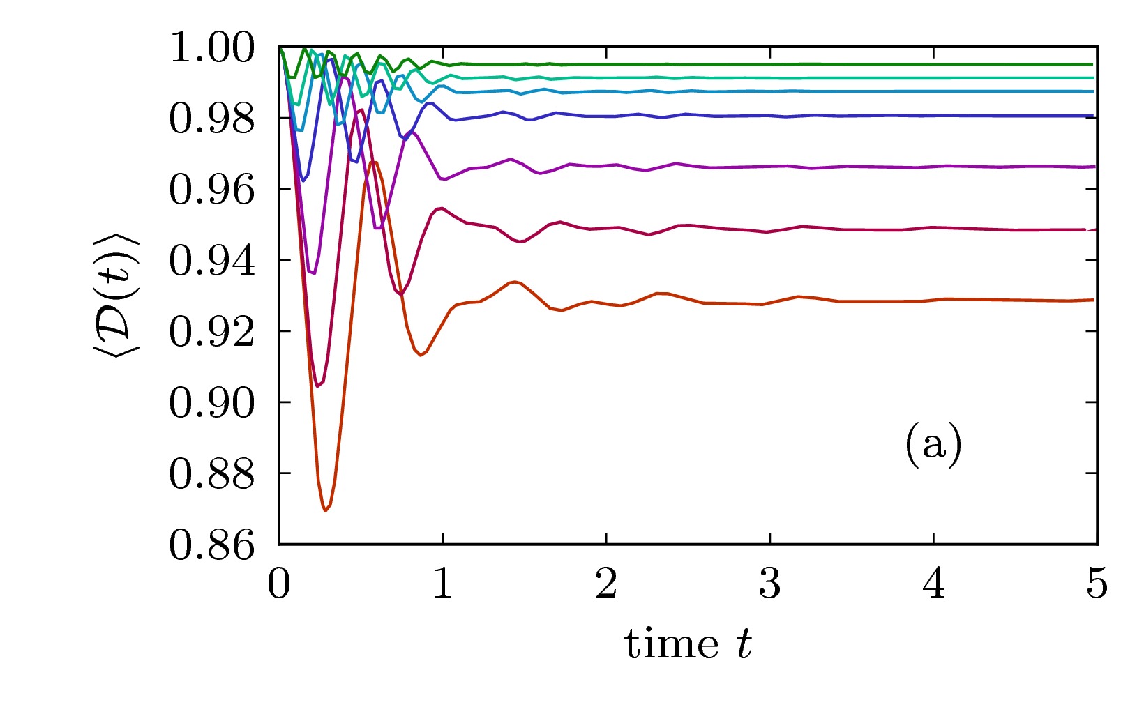
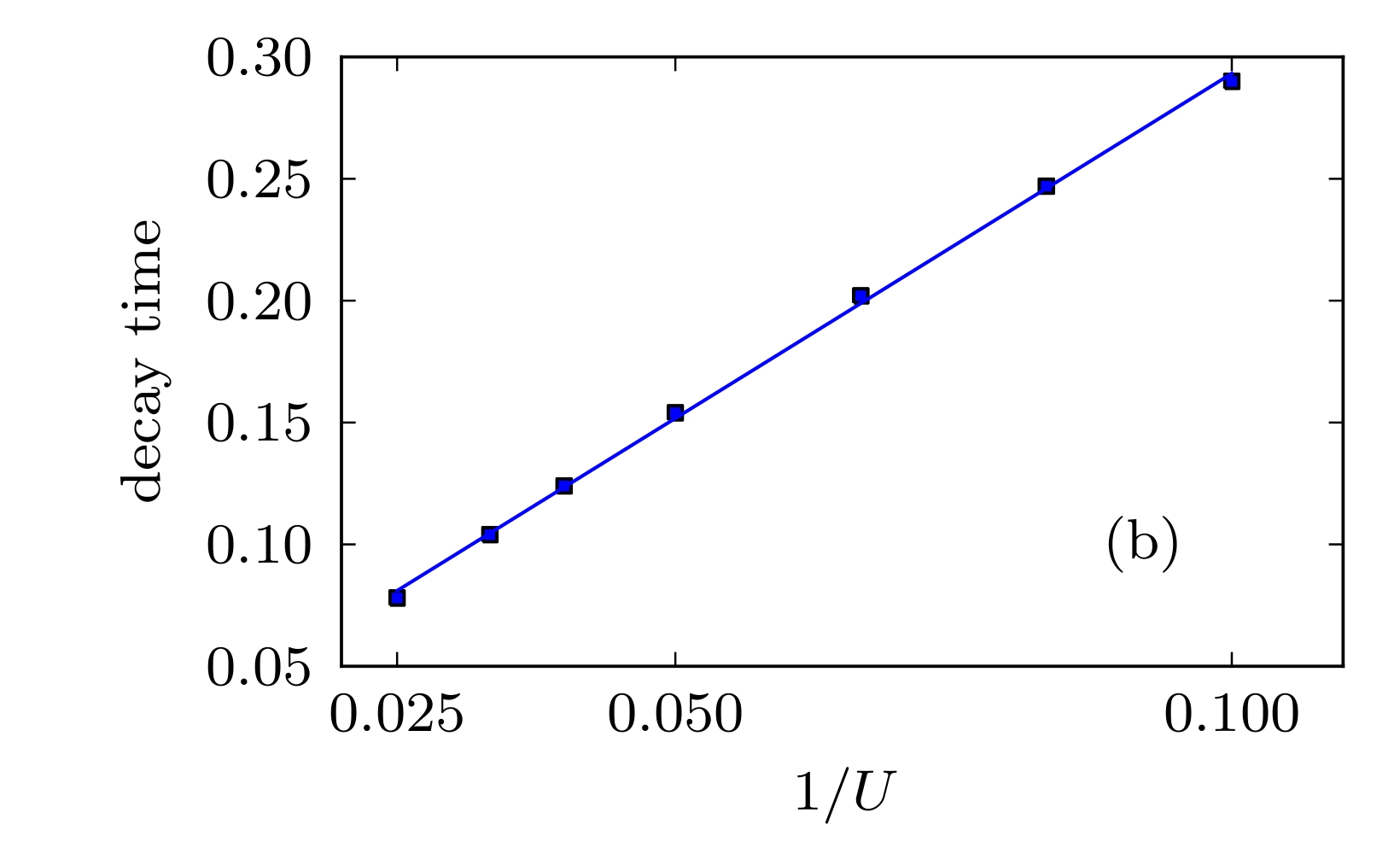
Figure 3: (a) Short-time behavior of the total double occupancy for $U=10,12,15,20,25,30,40$ (from bottom to top) and $V=0$. (b) First local minimum point (“decay time”) of the time-dependent total double occupancy plotted against $1/U$. The line is a guide to the eye.

The question how the observed doublon decay is consistent with energy conservation, is easily answered by means of time-dependent perturbation theory in $J$. For $J=0$, the total double occupancy is conserved. This already explains the high and nearly constant $\langle\mathcal{D}(t)\rangle$ for very strong $U$ [see the result for $U=40$ in Fig. 3(a)]. For strong but finite $U$ first-order-in-$J$ time-dependent perturbation theory predicts the transition probability between two unperturbed energy eigenstates $|\psi_{m}\rangle$ and $|\psi_{n}\rangle$ to behave as sakurai1993modernqm

$$\left|\langle\psi_{n}|e^{-i\mathcal{H}t}\psi_{m}\rangle\right|^{2}\propto\frac{\sin^{2}\left(\frac{\Delta E_{m\rightarrow n}}{2}t\right)}{(\Delta E_{m\rightarrow n})^{2}}\,.$$ (5)

This reminds us that “energy conservation” as used in the argument given at the beginning of the section holds in the long-time limit only where the right-hand side of Eq. (5) evolves into a $\delta$ function.

Doublon decay is possible (i) at short times or (ii) at long times and consistent with energy conservation in the presence of additional degrees of freedom to dissipate the excess energy. Let us discuss the case (i) first [see Sec. IX for point (ii)]: As a function of the energy difference $\Delta E_{m\rightarrow n}$, the transition probability has a peak structure with a width that scales as $1/t$. Hence transitions are possible between states with energy difference $\Delta E_{m\rightarrow n}\lesssim 1/t$. To put it in other words, excitations with energy $\Delta E_{m\rightarrow n}$ most probably occur on a time scale $t\lesssim 1/\Delta E_{i\rightarrow j}$. Therefore, since the dissociation of two fermions in the strong-coupling regime involves energies of the order of $U$, the position of the first minimum must scale with $1/U$, as demonstrated in Fig. 3(b).

At very short times, the decay is independent of the coupling $U$, as seen in Fig. 3(a) for $t\lesssim 0.2$. This is easily explained by Taylor expansion in $t$:

$$\langle\mathcal{D}(t)\rangle=1-t^{2}\>\Delta E_{\rm ini}+{\cal O}(t^{4})\;,$$ (6)

where the variance of the total energy in the initial state is proportional to the number of nearest neighbors $z=2$,

$$\Delta E_{\rm ini}=\langle\psi_{\text{ini}}|\mathcal{H}^{2}|\psi_{\text{ini}}\rangle-\langle\psi_{\text{ini}}|\mathcal{H}|\psi_{\text{ini}}\rangle^{2}=2zJ^{2}\;,$$ (7)

and thus depends on the hopping amplitude $J$ only.

VI Doublon dynamics and appearance-potential spectroscopy

The time-dependent expectation value of the double occupancy at site $i$ is

$$\langle\mathcal{D}_{i}(t)\rangle=\langle 0|\hat{d}^{\phantom{\dagger}}_{i_{0}}e^{i\mathcal{H}t}\hat{d}^{\dagger}_{i}\hat{d}^{\phantom{\dagger}}_{i}e^{-i\mathcal{H}t}\hat{d}^{\dagger}_{i_{0}}|0\rangle=\big{|}\langle 0|\hat{d}^{\phantom{\dagger}}_{i}e^{-i\mathcal{H}t}\hat{d}^{\dagger}_{i_{0}}|0\rangle\big{|}^{2}\,,$$ (8)

if a doublon has been prepared at $t=0$ at the site $i_{0}$, i.e., $\hat{d}^{\dagger}_{i}|0\rangle=\hat{c}^{\dagger}_{i\uparrow}\hat{c}^{\dagger}_{i\downarrow}|0\rangle$. Note that the original expectation value can be written as a square since (i) $\mathcal{H}$ commutes with the total particle number and (ii) we start from the Fermi vacuum. Namely, starting from the vacuum state $|0\rangle$, preparing of the doublon at site $i_{0}$, time propagation and finally annihilation at $i$, we must return to the same state $|0\rangle$.

The Fermi vacuum corresponds to an empty band in the context of electron spectroscopy. Let us discuss the relation of doublon dynamics to appearance-potential spectroscopy (APS),park1974softxrayaps ; ertl1993spinressoftxrayaps ; rangelov2000surfacemagneticprop in particular. Consider the following retarded two-particle (two-electron) Green’s function:

$$G_{ii,i_{0}i_{0}}(t)=-i\Theta(t)\langle 0|\hat{d}^{\phantom{\dagger}}_{i}e^{-i\mathcal{H}t}\hat{d}^{\dagger}_{i_{0}}|0\rangle\>.$$ (9)

This is a ground-state quantity, the Fourier transform of which, $G_{ii,jj}(\omega+i0^{+})=\langle\negthinspace\langle\hat{c}^{\phantom{\dagger}}_{i\uparrow}\hat{c}^{\phantom{\dagger}}_{i_{\downarrow}};\hat{c}^{\dagger}_{j\downarrow}\hat{c}^{\dagger}_{j\uparrow}\rangle\negthinspace\rangle_{\omega}$, yields the appearance-potential spectrum $A_{ii,ii}(\omega)=-\mbox{Im}G_{ii,ii}(\omega+i0^{+})/\pi$.potth2001theor $A_{ii,ii}(\omega)$ describes the cross section in a non-radiative two-electron process where an initial electron at high kinetic energy occupies an empty state in the valence band of a metal by transferring the energy difference to a core electron which is lifted to another empty state in the band. The process is essentially local and represents the “time inverse” of high-resolution core-valence-valence (CVV) Auger-electron spectroscopy.

For an empty band, the equation of motion for the APS Green’s function is readily solved:nolting1990influence

$$G_{ii,jj}(\omega+i0^{+})=\frac{1}{L}\sum_{\bm{k}}e^{i\bm{k}(\bm{R}_{i}-\bm{R}_{j})}\frac{\Lambda_{\bm{k}}(\omega+i0^{+})}{1-U\Lambda_{\bm{k}}(\omega+i0^{+})}\,,$$ (10)

with

$$\Lambda_{\bm{k}}(\omega)=\frac{1}{L}\sum_{\bm{p}}\frac{1}{\omega-\varepsilon(\bm{p})-\varepsilon(\bm{k}-\bm{p})}\;.$$ (11)

Here $\bm{R}_{i}$ denotes the position vector to the site $i$, $\bm{k}$ is a wave vector of the first Brillouin zone, and the dispersion of the tight-binding band $\varepsilon(\bm{k})=-J\sum_{\bm{\Delta}}\exp(-i\bm{k}\bm{\Delta})$ is obtained as a sum over nearest-neighbors displacement vectors $\bm{\Delta}$.

For $t>0$ we have $\langle\mathcal{D}_{i}(t)\rangle=|G_{ii,i_{0}i_{0}}(t)|^{2}$ and thus

$$\langle\mathcal{D}_{i}(t)\rangle=\left|\frac{1}{2\pi}\int d\omega\>e^{-i\omega t}G_{ii,i_{0}i_{0}}(\omega+i0^{+})\right|^{2}\>.$$ (12)

At $U=0$ this related to the Bessel function, $\left<\mathcal{D}_{i}^{\text{free}}(t)\right>=\mathcal{J}_{i-i_{0}}^{4}(2Jt)$. For $U>0$, and using the fact that the Green’s function is the Hilbert transform of the spectral function, we find

$$\langle\mathcal{D}_{i}(t)\rangle=\int d\omega\int d\omega^{\prime}e^{i(\omega-\omega^{\prime})t}A_{i_{0}i_{0},ii}(\omega)A_{ii,i_{0}i_{0}}(\omega^{\prime})\>.$$ (13)

After substituting $\omega\mapsto\omega+\omega^{\prime}$, we see that the time dependence of the local double occupancy is given by the Fourier transform from frequency to time representation of the self-convolution of the APS spectral function. This relation is remarkable as it provides a link between the APS spectral function, an equilibrium quantity describing two-particle excitations within the framework of linear-response theory, and the non-equilibrium time evolution of the local double occupancy. It is by no means general, however, and can be traced back to Eq. (8) which holds in the case of an empty band only.

VII Decay of a doublon — long-time stability

In the long-time limit, for an infinitely large system, i.e., $L\to\infty$, the local double occupancy $\langle\mathcal{D}_{i}(t)\rangle\to 0$ for $t\to\infty$ due to a complete delocalization of the doublon or the two independent fermions, respectively. The total double occupancy $\langle\mathcal{D}(t)\rangle$, however, may relax to a finite value. Still there are temporal fluctuations of $\langle\mathcal{D}(t)\rangle$ as $[\mathcal{D},\mathcal{H}]\neq 0$; see Fig. 3(b) and also Fig. 2, for examples. However, the fluctuations can be quite small as compared with the time average

$$\overline{\mathcal{D}}=\lim_{T\to\infty}\frac{1}{T}\int_{0}^{T}dt\>\langle\mathcal{D}(t)\rangle\,.$$ (14)

To quantify these observations, the time average after the initial decay at short times as well as the relative standard deviation $(\overline{\mathcal{D}^{2}}-\overline{\mathcal{D}}^{2})^{1/2}/\overline{\mathcal{D}}$, as a measure for the temporal fluctuations, are shown as contour plots in Fig. 4. Some sectional views are given in Fig. 5.

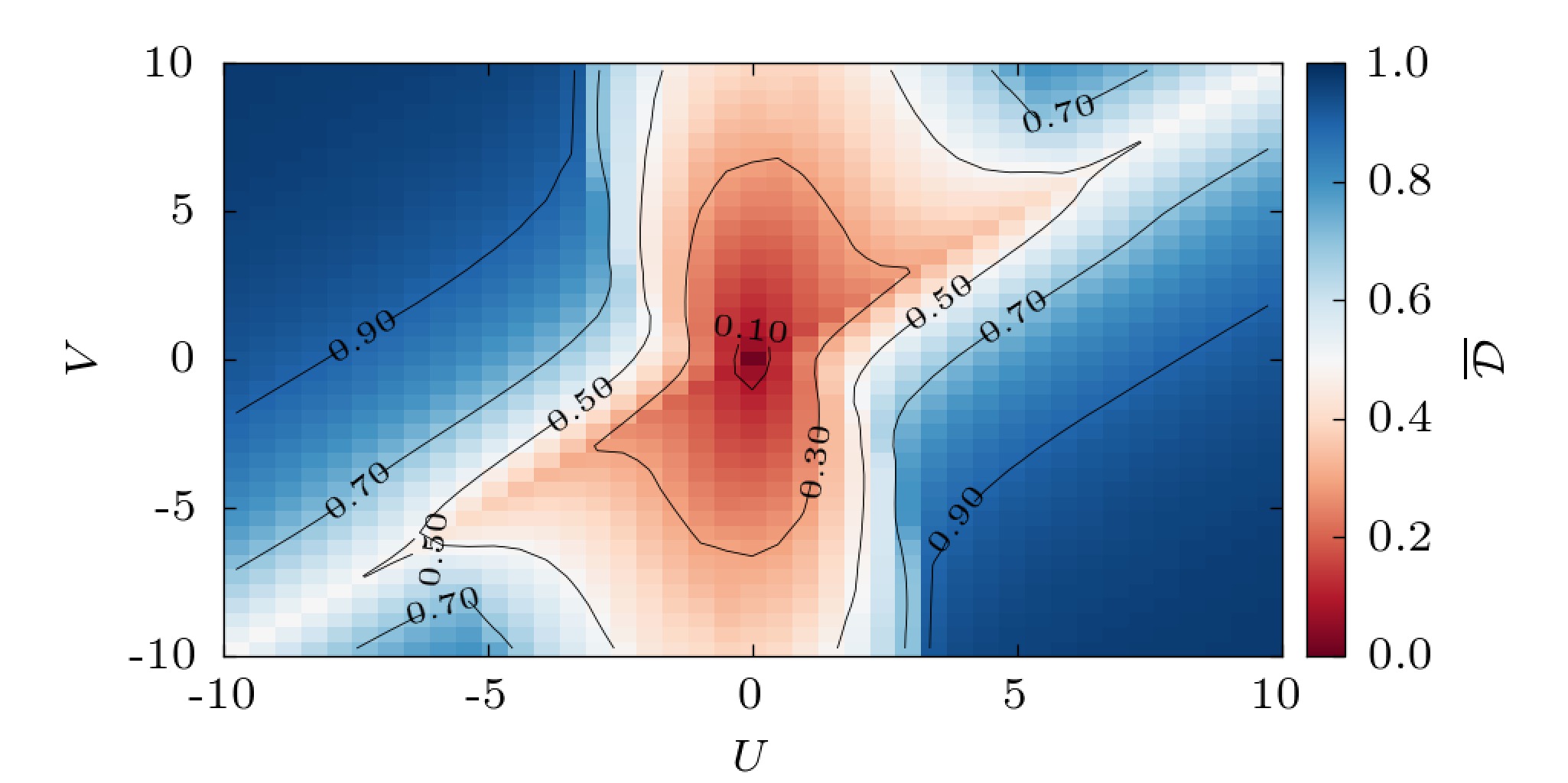
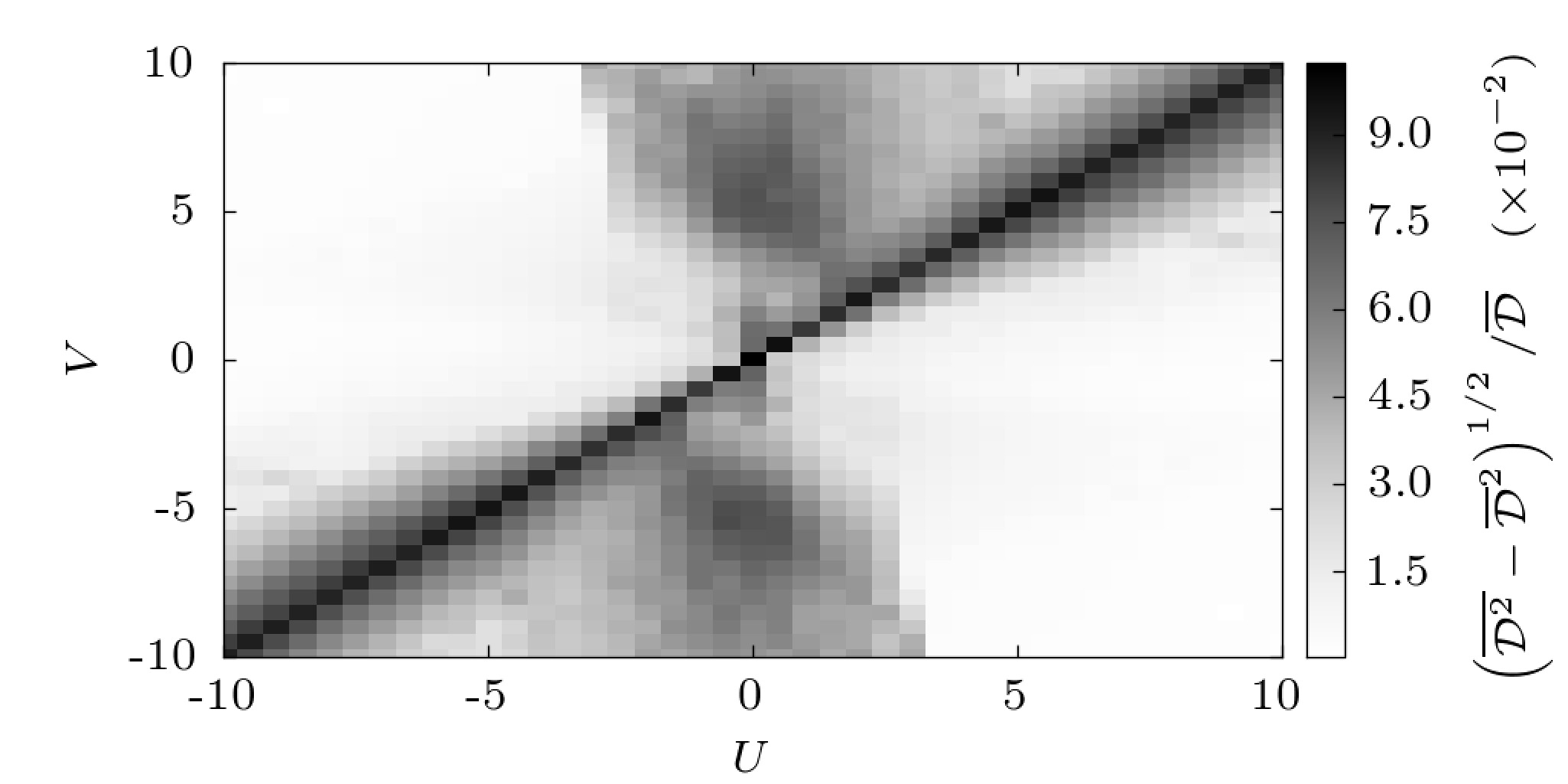
Figure 4: Long-time average (top) and relative standard deviation (bottom) of the total double occupancy $\langle\mathcal{D}(t)\rangle$ for interaction strengths $-10<U<10$ and $-10<V<10$. $\overline{\mathcal{D}}$ and $(\overline{\mathcal{D}^{2}}-\overline{\mathcal{D}}^{2})^{1/2}/\overline{\mathcal{D}}$ are calculated for the time interval $50<t<100$. The color or grey-scale code is given on the right.

For vanishing couplings $U$ and $V$ the doublon decays on a short-time scale and is found anywhere in the lattice with a probability of approximately $0.019$ (for $L=100$) at later times but fluctuations are strong. For finite and increasing $U$, but keeping $V=0$, the doublon stability rapidly rises while the relative fluctuations decrease. This is understood easily as the energy conservation described by Eq. (5) becomes strict in the long-time limit, i.e., a single doublon in an otherwise empty band is completely stable.remark

Using Eq. (13), we find the time average for $T\to\infty$,

$$\overline{\mathcal{D}}\propto\sum_{i}\int d\omega A_{i_{0}i_{0},ii}(\omega)A_{ii,i_{0}i_{0}}(\omega)\,,$$ (15)

to be given by the integrated square of the nonlocal APS spectral density. As $A_{ii,i_{0}i_{0}}(\omega)$ consists of a finite number of $\delta$ peaks for any finite $L$, the integral in Eq. (15) is ill defined. However, one can also compute $\overline{\mathcal{D}}$ directly, starting from Eq. (8), inserting resolutions of the unity in the form $\bm{1}=\sum_{m}|m\rangle\langle m|$ where $|m\rangle$ is the $m$th eigenstate of $\mathcal{H}$. Assuming the energy spectrum to be non-degenerate and assuming that there is relaxation at all, we easily find

$$\overline{\mathcal{D}}=\sum_{i}\sum_{m}\big{|}\langle 0|\hat{d}^{\phantom{\dagger}}_{i_{0}}|m\rangle\big{|}^{2}\big{|}\langle 0|\hat{d}^{\phantom{\dagger}}_{i}|m\rangle\big{|}^{2}\>.$$ (16)

With the expressions Eqs. (10) and (12) for the corresponding Green’s function, and using its Lehmann representation, this is also seen to be consistent with Eq. (15). Equation (15) provides the long-time “thermal” value of the total double occupancy.

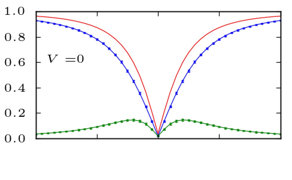
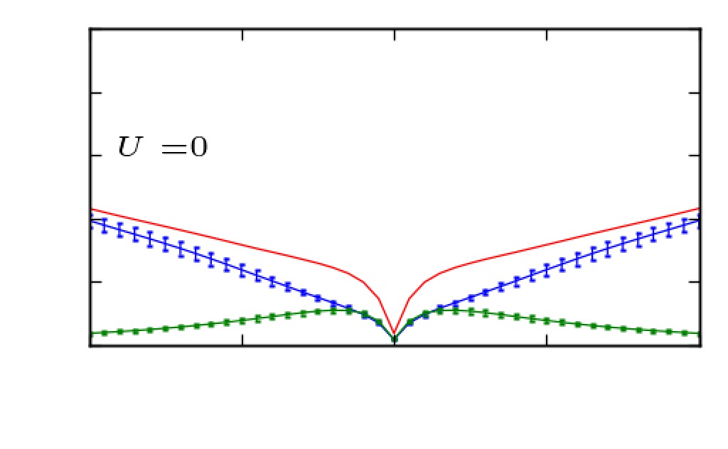
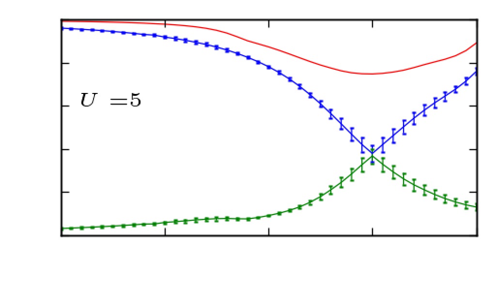
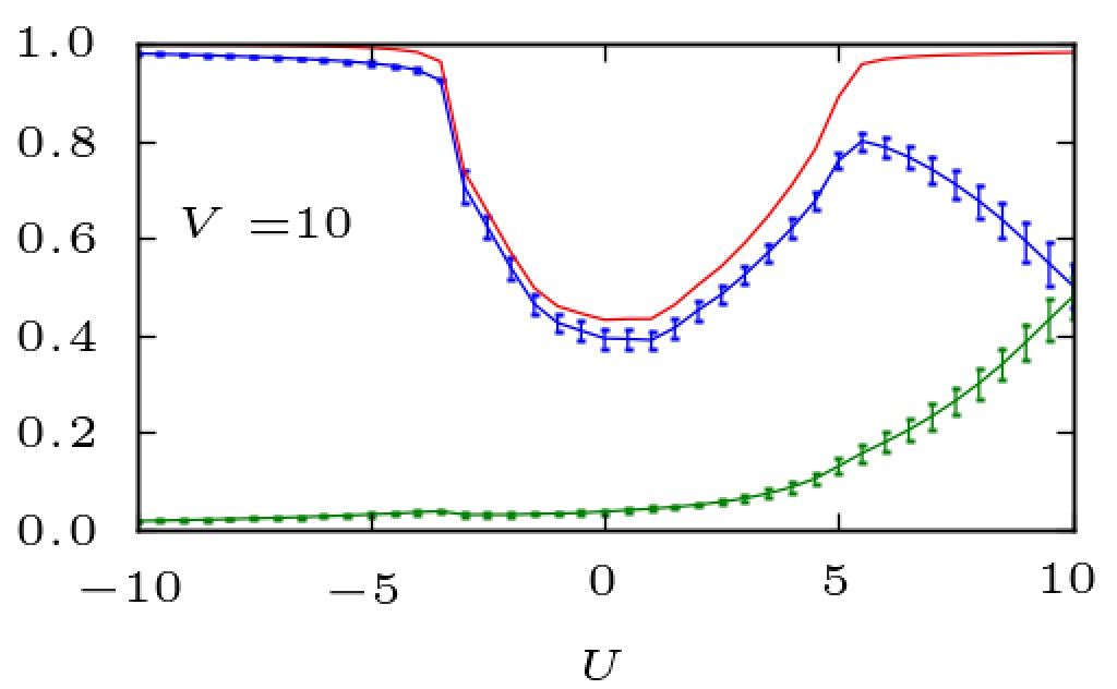
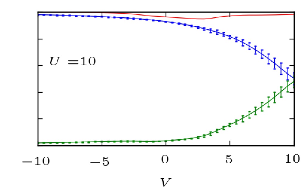
Figure 5: Sectional views of the stability map Fig. 4 for $U,V=0,5,10$. Blue lines show $\overline{\mathcal{D}}$, error bars indicate the absolute standard deviation. Green lines with error bars: time average and standard deviation of the nearest-neighbor occupancy, $\langle\frac{1}{2}\sum_{<ij>}\sum_{\sigma\sigma^{\prime}}\hat{n}^{c}_{i\sigma}(t)\hat{n}^{c}_{j\sigma^{\prime}}(t)\rangle$. Red: sum of double and nearest-neighbor occupancy.

For large $U$, the numerical results of Fig. 4 can be perfectly fitted by

$$\overline{\mathcal{D}}\simeq 1-\frac{m}{U^{2}}\;,$$ (17)

with the constant $m>0$ as a parameter. This behavior can be understood by perturbative arguments using the canonical transformation discussed in Sec. III and Appendix B: Using the unitary transformation $\mathcal{H}^{\prime}=e^{i\mathcal{S}}\mathcal{H}e^{-i\mathcal{S}}$ with the generator $\mathcal{S}$, we find

$$\langle\mathcal{D}(t)\rangle=\langle 0|\hat{d}^{\phantom{\dagger}}_{i_{0}}e^{-i\mathcal{S}}e^{i\mathcal{H}^{\prime}t}e^{i\mathcal{S}}\mathcal{D}e^{-i\mathcal{S}}e^{-i\mathcal{H}^{\prime}t}e^{i\mathcal{S}}\hat{d}^{\dagger}_{i_{0}}|0\rangle\,.$$ (18)

Exploiting particle-number conservation, we then get

$$\langle\mathcal{D}(t)\rangle=\sum_{i}\left|\langle 0|\hat{d}^{\phantom{\dagger}}_{i_{0}}e^{-i\mathcal{S}}e^{i\mathcal{H}^{\prime}t}e^{i\mathcal{S}}\hat{d}^{\dagger}_{i}|0\rangle\right|^{2}\,.$$ (19)

The state

$$|\psi^{\prime}_{i}\rangle\equiv e^{i\mathcal{S}}\hat{d}^{\dagger}_{i}|0\rangle=\hat{d}^{\dagger}_{i}|0\rangle+i[\mathcal{S},\hat{d}^{\dagger}_{i}]|0\rangle+{\cal O}(J^{2}/U^{2})$$ (20)

is a linear superposition of a one-doublon and a zero-doublon state

$$|\psi^{\prime}_{i}\rangle=|\psi^{\prime}_{i,1}\rangle-\frac{J}{U}|\psi^{\prime}_{i,0}\rangle+{\cal O}(J^{2}/U^{2})\,,$$ (21)

with $|\psi^{\prime}_{i,1}\rangle=\hat{d}^{\dagger}_{i}|0\rangle$ and $|\psi^{\prime}_{i,0}\rangle=-\sum_{k}^{\rm n.n.}(\hat{c}^{\dagger}_{k\uparrow}\hat{c}^{\dagger}_{i\downarrow}+\hat{c}^{\dagger}_{i\uparrow}\hat{c}^{\dagger}_{k\downarrow})|0\rangle$. This characteristic is, separately, preserved under the time evolution $e^{i\mathcal{H}^{\prime}t}$. After some algebra we find

$$\langle\mathcal{D}(t)\rangle = 1+\frac{J^{2}}{U^{2}}\sum_{i}\langle\psi^{\prime}_{i,1}|e^{-i\mathcal{H}_{\rm eff}t}|\psi^{\prime}_{i_{0},1}\rangle\langle\psi^{\prime}_{i_{0},0}|e^{i\mathcal{H}_{\rm eff}t}|\psi^{\prime}_{i,0}\rangle$$ (22)

$$+ \mbox{H.c.}+{\cal O}(J^{4}/U^{4})\,.$$

Hence perturbative in $1/U$ corrections to the total double occupancy are of the order $J^{2}/U^{2}$.

Equation (22) furthermore shows that in leading perturbation order there is a separation of characteristic time scales. The first matrix element involves energies in the one-doublon subspace and thus a short-time scale $1/U$. This is the time scale of the strong initial oscillations of $\langle\mathcal{D}(t)\rangle$, seen in Fig. 3, and once more explains the $1/U$ dependence of the “decay time,” i.e., the position of the first minimum. The second matrix element between states in the zero-doublon subspace provides a longer time scale $\sim 1/J$. This is the scale on which the oscillations decay. Finally, corrections to the $1/U$ scale are provided by effective doublon-hopping processes. This results in a scale $1/J^{\prime}\sim U/J^{2}$ the effects of which, however, are too weak to be seen in Fig. 3.

Finally, let us discuss the results for a finite nearest-neighbor interaction $V$. As is shown in Figs. 4 and 5, the initially prepared doublon is most unstable for $V\approx U$. Here, the transition $\hat{d}^{\dagger}_{i}\left|0\right>\rightarrow\hat{c}^{\dagger}_{i\uparrow}\hat{c}^{\dagger}_{i\pm 1,\downarrow}\left|0\right>$ becomes resonant. A further separation of the fermions beyond nearest-neighbor distances, however, is the more suppressed the larger $V$ gets. The latter is obvious for reasons analogous to those given above regarding the $U$ dependencies. As already noted in the context of propagation patterns above, for $U=V\neq 0$, an “extended doublon” is formed as a linear combination of a doubly occupied site with states where the two fermions are found at adjacent sites. Though the probability for finding two fermions at the same site anywhere in the lattice shows a minimum for $U=V$ in the stability map in Fig. 4, the one for finding them as nearest neighbors is almost equally large as can be seen in the sectional views of the stability map in Fig. 5. Furthermore, the sum of both equals the one for the same value of $U$ but vanishing $V$. At the same time the oscillations of the double occupancy as well as the one of nearest-neighbor state exhibit a maximum (Figs. 4 and 5) whereas their sum does not. Hence the oscillations cancel each other.

VIII Two doublons

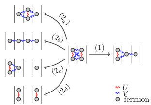
Figure 6: Scheme of dominant first-order [$(1)$, right] and second-order [$(2)$, left] hopping processes from an initial state with two doublons on nearest-neighbor sites to the possible final states. The involved interactions $U$ and $V$ are depicted by wiggly lines in red and blue, respectively.

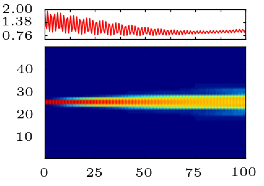
(a${}_{\text{nn}}$) $U=10,V=-10$

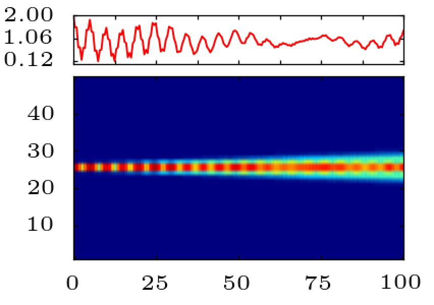
(b${}_{\text{nn}}$) $U=5,V=-10$

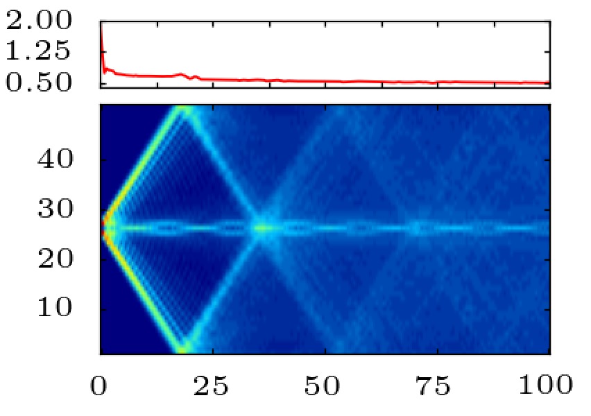
(a${}_{\text{nnn}}$) $U=5,V=5$

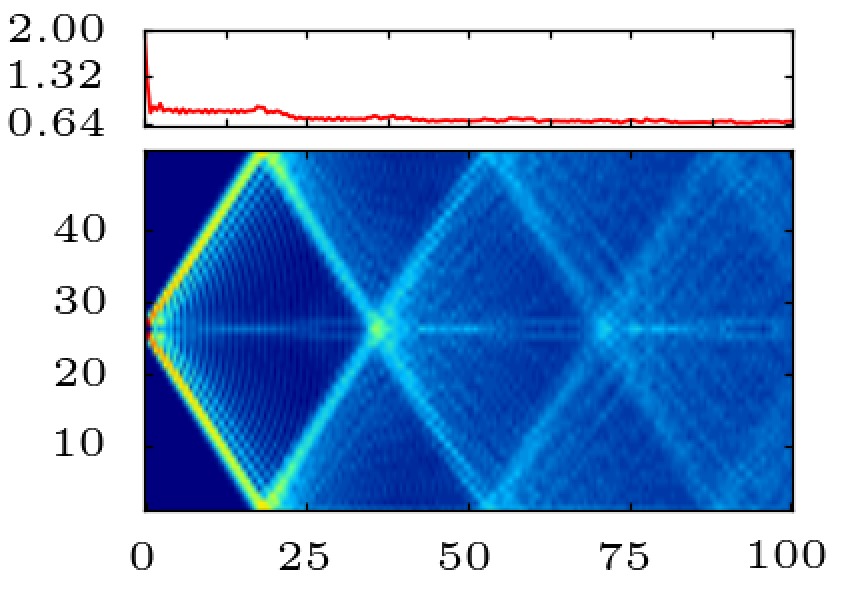
(b${}_{\text{nnn}}$) $U=10,V=10$

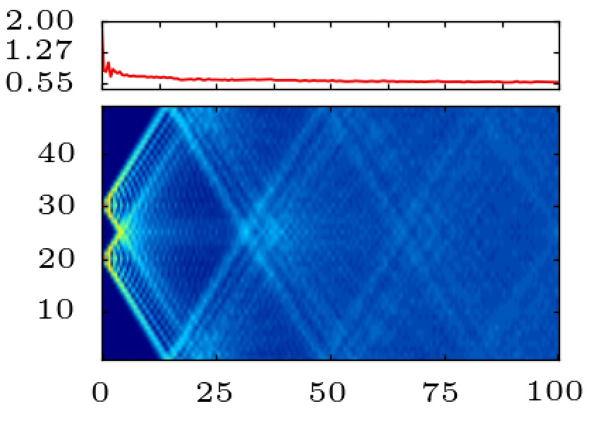
(a${}_{\text{sep}}$) $U=5,V=5$

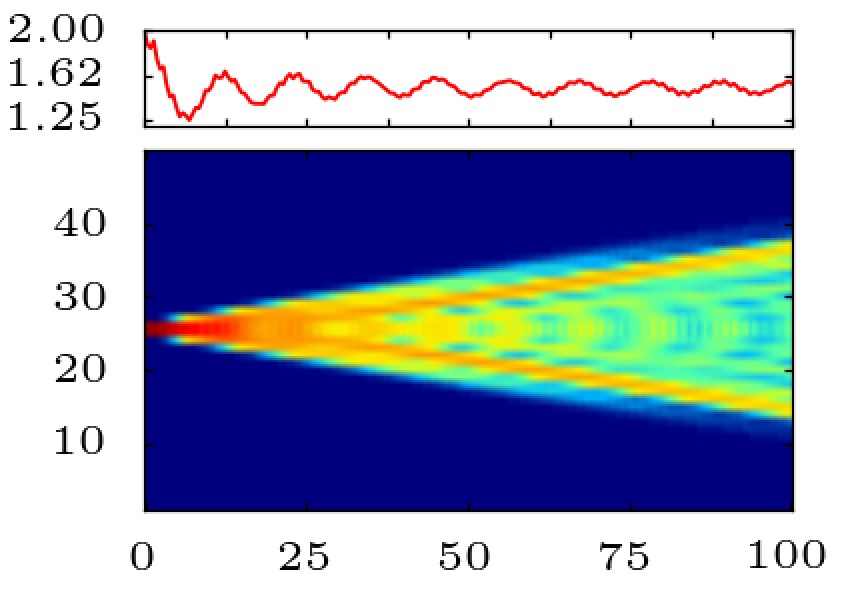
(c${}_{\text{nn}}$) $U=0,V=10$

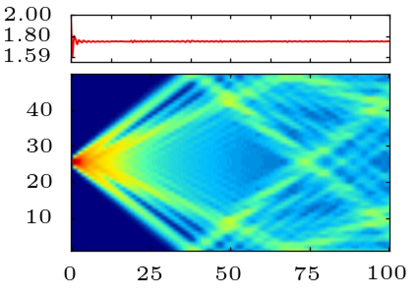
(d${}_{\text{nn}}$) $U=5,V=0$

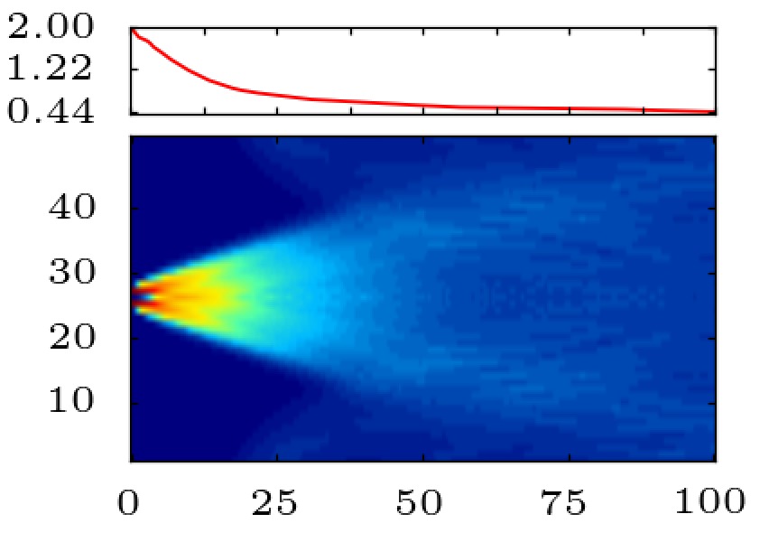
(c${}_{\text{nnn}}$) $U=0,V=10$

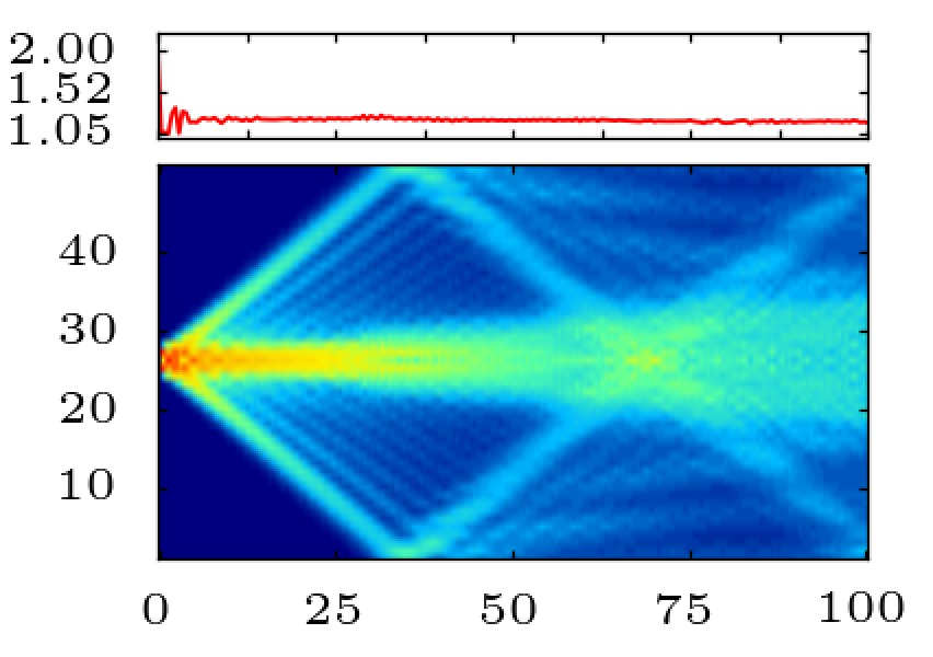
(d${}_{\text{nnn}}$) $U=6,V=2$

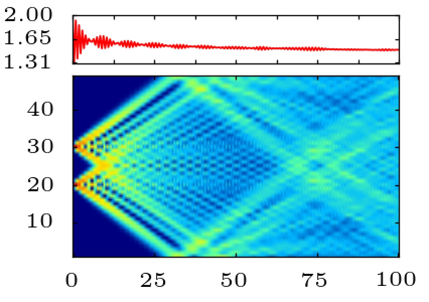
(b${}_{\text{sep}}$) $U=10,V=5$

(e${}_{\text{nn}}$) $U=10,V=-5$

(f${}_{\text{nn}}$) $U=10,V=10$

(e${}_{\text{nnn}}$) $U=8,V=2$

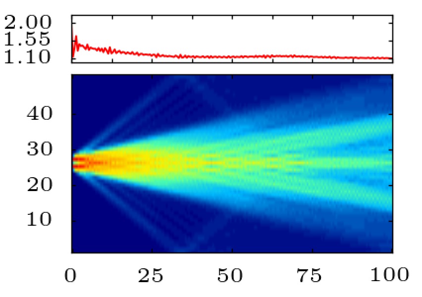
(f${}_{\text{nnn}}$) $U=8,V=4$

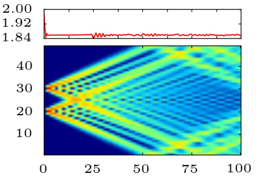
(c${}_{\text{sep}}$) $U=10,V=0$

Figure 7: Time dependence of the expectation value of the local (main panels) and the total double occupancy (small top panels) for different $U$ and $V$ as indicated. Axis and color code as in Fig. 1. Calculations are performed for different initial states as indicated by the bracketed symbols: two pairs fermions (two doublons) initially prepared as nearest-neighbors (x${}_{\text{nn}}$), next-nearest-neighbors (x${}_{\text{nnn}}$) or further separated with $|i-j|=10$ (x${}_{\text{sep}}$) respectively. Results for one-dimensional lattice with periodic boundary conditions and $L=50,51$ and $49$ sites, respectively.

The preceding examinations were restricted to the subspace of two fermions. This lacks some important aspects, such as doublon-doublon and doublon-fermion scattering. In the following we therefore extend our study to four-fermion states. The size of the one-dimensional lattice is fixed to $L\approx 50$.

VIII.1 Initial state with neighboring doublons

To begin with, consider an initial state at $t=0$ with two doublons at neighboring sites: $|\psi_{\text{ini}}\rangle=\hat{d}^{\dagger}_{i}\hat{d}^{\dagger}_{j}\left|0\right>$ with $|i-j|=1$. In the strong-coupling limit $U,V\gg J$, this state has a mean energy of the order of $2U+4V+{\cal O}(J^{2}/U,J^{2}/V)$: A state with two neighboring doublons entails two neighboring fermions for each constituent fermion. Processes starting from this state and involving a single or two hopping events will dominate the physics in the strong-coupling case and are sketched in Fig. 6.

Figure 7 shows the time-dependent local and total double occupancy for different $U$ and $V$. The overall trends can by understood by focusing on certain resonant cases as follows.

(i) If $V=-U$ the first order process, referred to as $(1)$ in Fig. 6, becomes resonant: The initial and final state have the same mean energy up to a small correction of the order ${\cal O}(J^{2}/U,J^{2}/V)$. In the strong-coupling limit a further spatial separation of the fermions is suppressed as there is a large excess energy $U$ or $V$ that cannot be accommodated in the system. A propagation of the compound object over many lattice sites is only possible via second-order hopping processes with a very low probability as compared to the first-order process (1). We therefore expect the two doublons to be basically localized at their initial positions. This explains the pattern shown in Fig. LABEL:sub@fig:two-nnU10V-10.

After some settling time the total double occupancy [see top panel in Fig. LABEL:sub@fig:two-nnU10V-10] tends to a value slightly less than unity which is less than expected for both states that define the process (1). We therefore conclude that there is a certain non-zero probability for the decay of the compound object into fragments without double occupancy that is not consistent with energy conservation. As discussed for the two-fermion case, this is possible at very short times.

The main dynamical effect, however, consists of a rapid oscillation between the two states of process (1). In the map for the time average $\overline{\mathcal{D}}$, see Fig. 8 (left), this manifests itself as a “valley” along the bisecting line of the second and fourth quadrant. Furthermore, this is accompanied by a maximum in the relative fluctuations (not shown), similar as in the two-fermion case.

(ii) Correspondingly, we find another “valley” along the line given by $V=-2U$ in Fig. 8 (left). This is associated with the second-order process $(2_{b})$ in Fig. 6 which is resonant here. Again, there is mainly an oscillation between the two states of $(2_{b})$ which both have the energy $2U+4V=3V$. The process involves a virtual intermediate state with an off-resonant energy $U+3V$.

As before in case (i), a propagation of the compound object over many lattice sites is suppressed as it necessarily involves fourth-order processes. In fact, Fig. LABEL:sub@fig:two-nnU5V-10 shows that the fermions essentially remain close to their initial sites.

An oscillation between the two states of $(2_{b})$ clearly implies the total double occupancy to oscillate between approximately $2$ and $0$. In the long-time limit it tends to relax to a value close to or slightly less than $1$.

(iii) In case of vanishing $U$, the second-order process $(2_{a})$ becomes resonant at the energy $2U+4V=4V$. This causes another branch of minima along the $V$ axis in Fig. 8 (left).

Opposed to cases (i) and (ii), the four-fermion cluster may propagate via the $(2_{a})$ process followed by a process inverse to $(2_{a})$ but resulting in two neighboring doublons shifted by one site to the left or right as compared with the initial state. Repeated second-order hopping processes then lead to a more efficient delocalization of the cluster and thus also of the expectation value for the double occupancy as is seen in Fig. LABEL:sub@fig:two-nnU0V10.

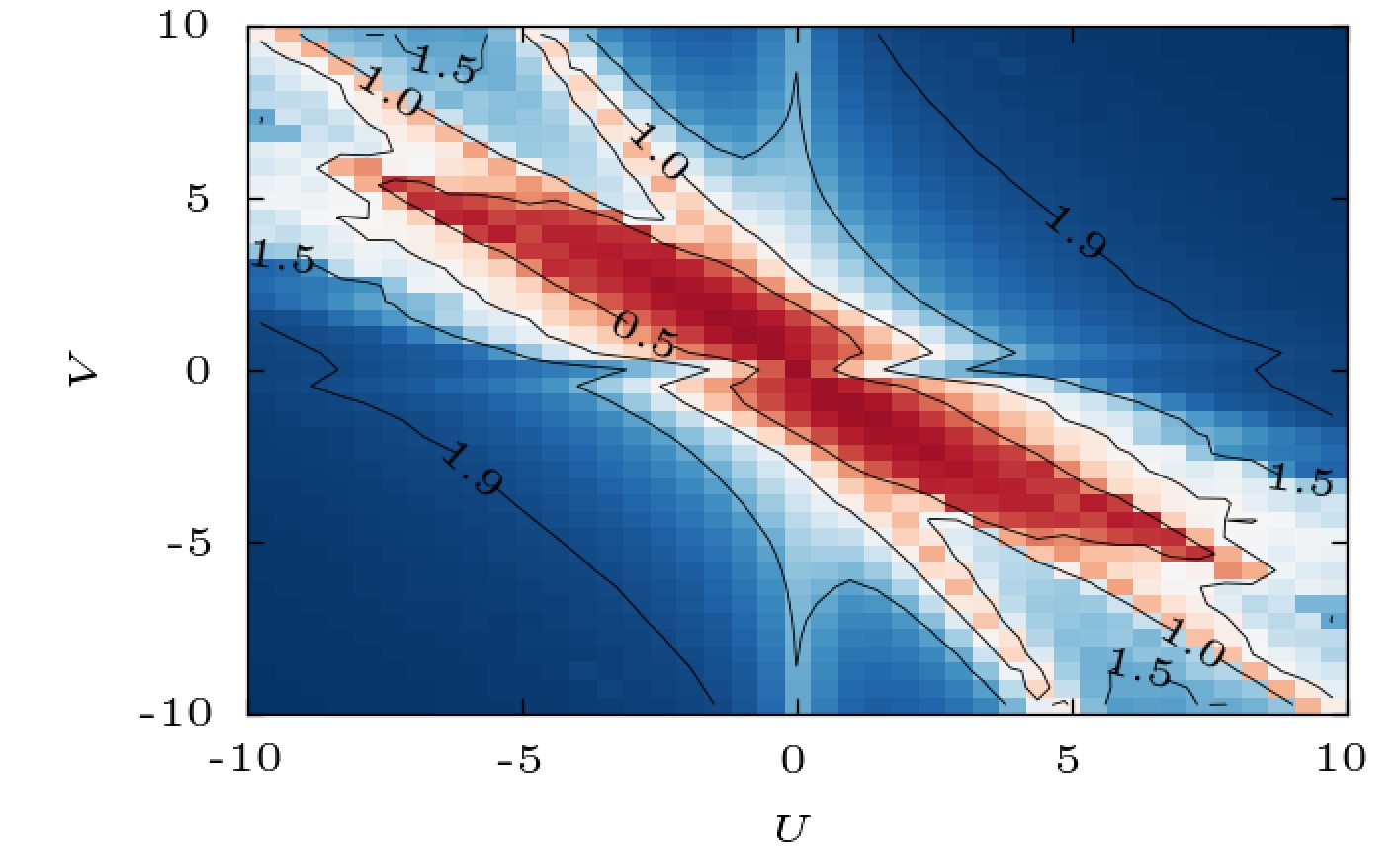
(a) nearest-neighbors

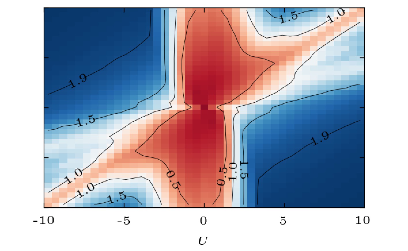
(b) next-nearest-neighbors

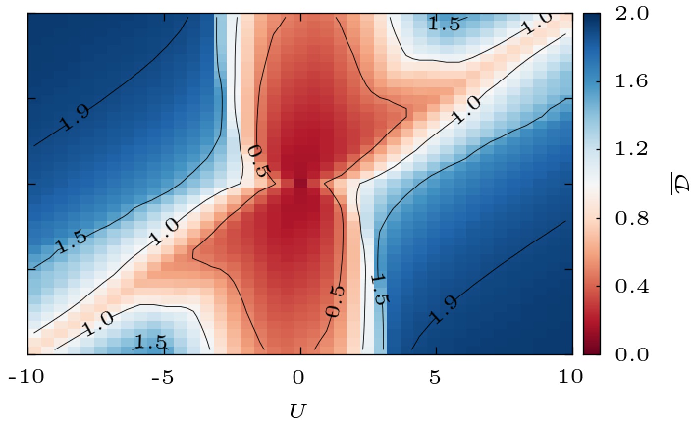
(c) further separated

Figure 8: Time average of the total double occupancy $\langle\mathcal{D}(t)\rangle$ for interaction strengths $-10<U<10$ and $-10<V<10$. Calculations for an initial state with two doublons placed at sites $i$ and $j$. (a) $i$ and $j$ nearest neighbors, (b) next-nearest neighbors and (c) $|i-j|=10$. Average over the time interval $50<t<100$. The color code is given on the right.

(iv) For a vanishing $V$, the process $(2_{d})$ becomes resonant at the energy $2U+4V=2U$. This implies that the initial cluster with two neighboring doublons can dissociate into two doublons separated at arbitrarily large distances via second-order hopping processes over off-resonant intermediate states. Delocalization is thus very efficient and results in the pattern displayed in Fig. LABEL:sub@fig:two-nnU5V0.

The propagation pattern is obviously dominated by two “light cones” with different velocities. This can be traced back to the interaction between the two doublons by comparing with the patterns in Figs. LABEL:sub@fig:two-sepU10V5 and LABEL:sub@fig:two-sepU10V0 which refer to an initial state where the two doublons are well separated and prepared at a distance $|i-j|=10$ and where the mode with lower velocity is absent. It is an open question whether the slow mode is due to the repulsive hard-core constraint or due to the attractive interaction in the effective Hamiltonian Eq. (2). The “light cone” associated with the higher velocity is identical to the one found for propagation of a single doublon, see Figs. LABEL:sub@fig:two-nnU5V0 and LABEL:sub@fig:oneU5V0 and mind the different lattice sizes.

In Fig. 8 (left), we find a signature of the resonant process $(2_{d})$ along the $V=0$ line. As in the two-fermion case, the doublons are stabilized with increasing $U$.

(v) Finally, the process $(2_{c})$ gets resonant if $2U+4V=U+2V$ which again becomes manifest in a valley, given by $V=-\frac{1}{2}U$, in the map, Fig. 8 (left), which is clearly visible at larger values of $U$ and $V$.

Regarding the mobility, we note that the process $(2_{c})$ can be either inverted or the fermion triple can move resonantly through the lattice. Both possibilities contribute to the propagation pattern shown in Fig. LABEL:sub@fig:two-nnU10V-5.

In all other cases, the initial state shows both a high stability and a marginal mobility in the strong-coupling limit. Figure LABEL:sub@fig:two-nnU10V10 gives an example for $U=V=10$. We note that the relative fluctuations around the time average amounts to approximately $1\%$ only.

VIII.2 Next-nearest neighbors

Although the underlying physics is the same, the results are completely different if the two doublons are prepared at sites which are next-nearest neighbors. The calculated propagation patterns are shown Fig. 7 in the third and fourth columns, while Fig. 8 (middle) displays the corresponding time averages. The dominant first-order and second-order hopping processes are sketched in Fig. 9.

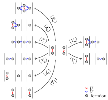
Figure 9: Scheme of dominant first-order [$(1^{\prime})$, right] and second-order [$(2^{\prime})$, left] hopping processes from an initial state with two doublons on next-nearest-neighbor sites to the possible final states. The inverse of process $(2_{d})$ (see Fig. 6) is not shown again. $U$ and $V$ are depicted by wiggly lines in red and blue, respectively.

First, we note that the processes $(1^{\prime}_{b})$, $(2^{\prime}_{d})$, $(2^{\prime}_{e})$, and $(2^{\prime}_{f})$ are all independent of the problem’s four-particle character. Provided that the physics is dominated by those processes, one would expect the propagation pattern of two initially next-nearest-neighboring doublons to essentially resemble that of two independent doublons. In the strong-coupling limit, this is the case for processes $(1^{\prime}_{b})$, $(2^{\prime}_{d})$ if $U=V$ and independently of $V$ for $(2^{\prime}_{f})$. As is seen Figs. LABEL:sub@fig:two-nnnU5V5 and LABEL:sub@fig:two-nnnU10V10, the doublons’ propagation is described by about the same maximal effective hopping as in the case of a single doublon; see Fig. LABEL:sub@fig:oneU10V10, for example. There is, however, an additional mode visible in Figs. LABEL:sub@fig:two-nnnU5V5 and LABEL:sub@fig:two-nnnU10V10 which results from the two doublons resting more or less at their initial sites. This is caused by the respective inverse hopping processes and basically disappears with increasing interaction strengths $U=V\to\infty$ and also in the case where the two doublons are prepared at a larger distance [see Fig. LABEL:sub@fig:two-sepU5V5]. A branch of minima occurs along the line $U=V$ in the stability map, Fig. LABEL:sub@fig:two_stab_nnn, which looks similar to that obtained in the two-fermion case (cf. Fig. 4). The process $(2^{\prime}_{e})$ is resonant only if $U=0$. Here the doublons rapidly dissociate into more or less independent fermions resulting in deep valley around $U=0$ in Fig. LABEL:sub@fig:two_stab_nnn.

The processes $(1^{\prime}_{a})$, $(2^{\prime}_{a})$, $(2^{\prime}_{b})$ and $(2^{\prime}_{c})$ are immanent to the four-particle character of the problem and become resonant if $V=\frac{1}{3}U$, $V=\frac{1}{4}U$, $V=\frac{1}{2}U$ or $V=\frac{2}{3}U$, respectively. The same holds for the inverse to process $(2_{d})$ (see Fig. 6) which becomes resonant if $V$ vanishes. Except for the last one, the doublon number is changed in all processes. We therefore expect and find a region of instability, bounded from below by $V=\frac{1}{4}U$ as can be seen from the level curves in Fig. LABEL:sub@fig:two_stab_nnn. Generally, the propagation patterns LABEL:sub@fig:two-nnnU6V2, LABEL:sub@fig:two-nnnU8V2 and LABEL:sub@fig:two-nnnU8V4 are not easily interpreted by means of simple perturbative arguments.

It is worth mentioning that for vanishing nearest-neighbor interaction $V=0$ (not displayed) the doublons essentially show the same spreading behavior as they did in the case of a single doublon [see Fig. LABEL:sub@fig:two-nnU5V0] and their stability again rises with $|U|$. Further, for large couplings of opposite sign $U=-V$, all processes except for $(2^{\prime}_{f})$ are strongly suppressed. The patterns (not displayed) are rather similar to those for a single doublon [see Fig. LABEL:sub@fig:two-nnU10V-10].

VIII.3 Further separation in the initial state

The further away two doublons are prepared in the initial state the less they influence each other. We therefore obtain results similar to those for a single doublon. This can be seen from our calculations with two doublons initially separated by ten sites by comparing, e.g., the maps for the long-time averages $\overline{\mathcal{D}}$, Figs. LABEL:sub@fig:two_stab_sep and 4, as well as by comparing the propagation patterns in Figs. 7 and 2 for corresponding interaction strengths.

VIII.4 Comparison with the bosonic case

Generally, the propagation patterns considerably differ from the corresponding ones for doublons formed by bosons. Motivated by experiment,winkler2006repulsivelybound Petrosyan et al. petrosyan2007quantumliquid consider the Bose-Hubbard model, $\mathcal{H}=-J\sum_{\left<ij\right>}\hat{b}^{\dagger}_{i}\hat{b}^{\phantom{\dagger}}_{j}+(U/2)\sum_{i}\hat{n}^{b}_{i}(\hat{n}^{b}_{i}-1)$, in the strong-coupling limit with an additional constraint excluding states, analogous to the Fermi case, with two or more bosons at the same site. Preparing an initial state with two neighboring doublons, propagation patterns are obtained which look very similar to our cases $U=-V=10$ or $U=V=10$ [see Figs. LABEL:sub@fig:two-nnU10V-10 and LABEL:sub@fig:two-nnU10V10], i.e., propagation is strongly suppressed. This can be understood by again referring to a respective effective model for the strong-coupling limit. Canonical transformation yieldspetrosyan2007quantumliquid

$$\mathcal{H}_{\text{eff}}=\frac{J^{\prime}}{2}\sum_{\left<ij\right>}\hat{d}^{\dagger}_{i}\hat{d}^{\phantom{\dagger}}_{j}\\ +(J^{\prime}+U)\sum_{i}\hat{n}^{d}_{i}-2J^{\prime}\sum_{\left<ij\right>}\hat{n}^{d}_{i}\hat{n}^{d}_{j}\,.$$ (23)

Here, $\hat{d}^{(\dagger)}_{i}$ denotes the annihilation (creation) operator for doublons made up of bosons $(\hat{b}^{(\dagger)})$. As in the Fermi case, the effective hopping is given by $J^{\prime}=4J^{2}/U$. Equation (23) should be compared with Eq. (2). In contrast to the fermionic case, the attractive interaction between two nearest-neighboring doublons is larger by a factor $4$ for doublons made of bosons. This explains the tendency to a strongly suppressed propagation.

It also explains that, in the bosonic case, the formation of clusters of doublons is favored and phase separation is possible below some critical temperature.petrosyan2007quantumliquid Contrary, in the Fermi case, doubly occupied sites may Bose condensate under certain circumstances.rosch2008metastable In fact, we did not find any indications for a clustering of doublons. Two doublons are rather never found to form a bound state unless an explicit nearest-neighbor interaction $V$ is present.

IX Doublon-fermion scattering

The propagation and the decay of a repulsively bound pair is expected to be strongly affected by the presence of additional fermions. As a finite fermion density cannot be studied reasonably by means of the Krylov approach, we will here consider two additional fermions only. To this end we first determine the ground state of the Hamiltonian in the two-fermion subspace $\left|\Omega_{2}\right>$ and subsequently add a doublon at a certain site $i_{0}$ to define the initial state $\hat{d}^{\dagger}_{i_{0}}\left|\Omega_{2}\right>$. Since the weight of doubly occupied sites in the ground state is almost vanishing for a lattice with $L=50$ sites, this setup allows us to study the scattering of the doublon with almost independently propagating fermions.

Here we focus on the decay of the doublon for the $V=0$ case only but consider different initial states. Besides $\hat{d}^{\dagger}_{i_{0}}\left|\Omega_{2}\right>$, we also study the system’s time evolution starting from states where two fermions are prepared at sites close to the initial position of the doublon $i_{0}$, i.e. $|m,m^{\prime}\rangle\equiv\hat{c}^{\dagger}_{i_{0}+m\uparrow}\hat{d}^{\dagger}_{i_{0}}\hat{c}^{\dagger}_{i_{0}-m^{\prime}\downarrow}|0\rangle$. This is compared to results obtained for two doublons at nearest-neighboring sites, $\hat{d}^{\dagger}_{i_{0}}\hat{d}^{\dagger}_{i_{0}+1}|0\rangle$, and two doublons prepared at a distance of 2 and 10, i.e. $\hat{d}^{\dagger}_{i_{0}}\hat{d}^{\dagger}_{i_{0}+2}|0\rangle$ and $\hat{d}^{\dagger}_{i_{0}}\hat{d}^{\dagger}_{i_{0}+10}|0\rangle$, respectively. In all cases we find a decay of the doublon expectation value on a short-time scale $1/U$ followed by a stabilization to a nearly constant value at large times. The residual quantum fluctuations are disregarded by looking at the time average $\overline{\mathcal{D}}$. As before, we find that the decayed doublon fraction scales linearly with $1/U^{2}$ for large times, $\overline{\mathcal{D}(t)}\simeq\langle\mathcal{D}(0)\rangle(1-m/U^{2})$. Hence in the strong-coupling limit the doublon stability is quantified by the coefficient $m$. For $m=0$ there is no decay at all, and a small value for $m$ indicates a rather stable doublon. Our results for the different initial states are shown in Fig. 10.

Figure 10: Coefficient $m$ obtained from a fit of the time-averaged expectation value for the total double occupancy $\overline{\mathcal{D}(t)}$ to the observed $U$ dependence: $\overline{\mathcal{D}(t)}\simeq\langle\mathcal{D}(0)\rangle(1-m/U^{2})$. $m$ values are obtained from linear regression of our data in the range $8\leq U\leq 45$. Results are shown for different initial states as indicated and discussed in the text. $n=1$ refers to the results of a time-dependent DMRG calculation by Al-Hassanieh et al., see Ref. hassanieh2008excitonsin1dhubbard, and text for discussion.

Generally, for a system with additional fermions, one expects an hugely increased phase space for inelastic processes leading to doublon decay. On the other hand, the energy-conservation argument suggests that for strong $U$ a rather complex inelastic process has to take place to allow for decay, namely a process of high order where a sufficient number of particles must be involved to dissipate a large energy of the order of $U$. While such processes are expected to be exponentially suppressed for large $U$, they should contribute to some degree and lead to a destabilization of a doublon.

However, our results for different initial states, as displayed in Fig. 10, just show the opposite trend: The presence of two additional fermions in the initial state in all cases leads to a smaller coefficient $m$ in the $1/U^{2}$ decay law. The strongest effect is visible for the initial state $|1,1\rangle$ where the two fermions are neighbors of the doublon at $i_{0}$. Here $m$ is the smallest and the doublon is most stable. $m$ increases with increasing distance of one of the fermions from the position of the doublon; see the initial states $|1,2\rangle$ and $|1,3\rangle$. It further increases if also the second fermion is positioned at a distance from $i_{0}$ (see $|2,2\rangle$, $|3,3\rangle$, and $|4,4\rangle$), and it approaches the value obtained for the case where both fermions are delocalized in the ground state $\hat{d}^{\dagger}_{i_{0}}\left|\Omega_{2}\right>$. The maximum value is obtained for the isolated doublon in an otherwise empty lattice, i.e., for $\hat{d}^{\dagger}_{i_{0}}|0\rangle$. If the two fermions themselves form a second doublon, see the results for $\hat{d}^{\dagger}_{i_{0}}\hat{d}^{\dagger}_{i_{0}+x}|0\rangle$ in Fig. 10, this again tends to stabilize the original one: $m$ decreases with decreasing distance $x$ between the two doublons.

These trends can be understood if the doublon dynamics is considered at short times: First-order-in-$J$ time-dependent perturbation theory shows that doublon decay is allowed on a time scale $1/U$ as has been detailed in Sec. V. Here, one can argue that an unoccupied site neighboring the doublon is necessary for the decay process as the immediate surrounding is relevant for its start. Hence, the coefficient $m$ is the smaller and the doublon is more stable if decay channels are blocked by localized fermions or doublons close to the doublon at $i_{0}$ and, to a lesser extent and depending on the size of the lattice, even by two delocalized fermions in the two-fermion ground state. This nicely explains the results described above.

After that time scale, energy conservation as expressed by Fermi’s golden rule, applies and the total double occupancy virtually relaxes to a constant value. As analyzed in Sec. VII, the probability for the dissociation of a doublon should then scale as $1/U^{2}$. On an for large $U$ extremely long time scale, which exponentially depends on $U$,strohmaier2010observationdoublondecay contributions from higher-order perturbation theory in $J/U$ become important and would generally allow for further decay in more complex processes.hansen2011splithubbardbands

In this context it is interesting to compare our results with the those of a time-dependent density-matrix renormalization-group (DMRG) study by Al-Hassanieh et al. hassanieh2008excitonsin1dhubbard where the decay of a doublon created by a nearest-neighbor particle-hole excitation of a half filled one-dimensional Fermi Hubbard model was considered. The DMRG calculations show (i) a fast decay at a characteristic time scale $1/U$, (ii) a basically constant double occupancy at larger times up about 40$J^{-1}$, and (iii) a $1/U^{2}$ scaling of the decayed fraction of the doublon. All this agrees perfectly with our results obtained for four fermions only. The $m$ coefficient taken from the DMRG results hassanieh2008excitonsin1dhubbard is also included in Fig. 10 (“$n=1$”) and is found to be close to that obtained for the $|1,2\rangle$ initial state. Even this is plausible since the spin-dependent site occupations of the state $|1,2\rangle$ and of the initial state of the DMRG calculation are the same in the immediate environment of $i_{0}$.

The at least qualitative agreement with the dynamics of the half filled model on the time scale accessible to time-dependent DMRG appears as surprising at first sight: Clearly, the initial local blocking of decay channels is the same in the four-fermion and in the half filled case but this would only explain an agreement on a time scale much shorter than the one accessible by DMRG. We suggest that it is important to take into account an additional argument here, namely, the fact that decay of the doublon on intermediate time scales larger than $1/U$ is basically ruled out by energy conservation while on time scales shorter than $1/U$ it is only the immediate surrounding of the doublon that counts. This would explain the almost quantitative agreement with the DMRG results of Ref. hassanieh2008excitonsin1dhubbard, .

On the other hand, this argument leaves the possibility for an, e.g., exponential-in-$t$ decay law on much larger time scales. hansen2011splithubbardbands ; strohmaier2010observationdoublondecay This might be expected on general grounds as adding more degrees of freedom to the system should strongly increase the phase space available for decay in energy-conserving processes where the doublon energy $U$ is dissipated to a large number of particle-hole or spin excitations. Those processes, however, require a huge time scale to contribute significantly to the doublon decay, possibly well beyond the time scales accessible by DMRG.

Note that a quantitative comparison with the DMRG study of Ref. enss2011lightconerenorm, for the half filled Hubbard model is not possible, as an initial state where doubly occupied and empty sites alternate is considered there. Still the qualitative features are rather similar.

X Summary

Concluding, the real-time dynamics of two or a few more strongly interacting Fermions moving in a periodic lattice potential exhibits a surprisingly rich physics which is not only linked to experiments with ultracold atoms trapped in optical lattices but also to electron spectroscopy of metal surfaces as well as to rather general questions on the propagation and decay of bound quantum states and the relaxation of quantum systems prepared in a highly excited initial state. Here we have employed a Krylov-space method lanczos1950iteration ; park1986unitary ; saad1992analysiskrylovsubspaceapprox ; hochbruck1997krylov ; hochbruck1999exponentialintegrators ; molervanloan2003expmatrix ; manmana2005timev1d to study few-particle systems with a moderately large Hilbert-space dimension. Even the analysis of the two-fermion case helps us to understand important concepts such as the temporal stability of a doublon, i.e., a repulsively bound pair of fermions.

The decay of a doublon in an otherwise empty system is possible on a very-short time scale $1/U$ where energy conservation, within the spirit of time-dependent first-order perturbation theory, does not apply. Using perturbative diagonalization of the Hamiltonian by means of a canonical transformation, one can understand the observed $1/U^{2}$ dependence of the fraction of the doublon that has decayed in the long-time limit.

The time average of the total double occupancy is found to be given by a quantity defined for the equilibrium or ground state of the system, namely the integrated square of the spectral density related to appearance-potential spectroscopy. But also the fully time-dependent local double occupancy can be expressed in terms of this spectral function, which must be seen as an unexpected interrelation valid for a two-particle system only.

The spatiotemporal evolution of the expectation value of the local double occupancy can be understood by perturbative arguments, even in the case of a non zero nearest-neighbor interaction $V$. In the case of four fermions, the propagation patterns are much more complicated. Still, we could demonstrate that the real-time dynamics after preparation of different initial states can be understood in most but not all cases by perturbative arguments.

The physics of a finite density of doublons consisting of fermions is known to be rather different from the case of doublons made of bosonic particles which undergo a transition to a phase-separated state instead of Bose condensation.petrosyan2007quantumliquid ; rosch2008metastable Consistent with this, we did not find any indications for a clustering of doublons consisting of fermions unless an explicit nearest-neighbor-interaction $V$ is present.

Surprisingly, there is a rather regular trend concerning the decay of a single doublon in the presence of two more fermions. The total double occupancy, apart from quantum fluctuations, relaxes to a constant value after an initial decay on a time scale $1/U$, and the long-time average deviates from the initial value by a fraction that scales with $U$ as $1/U^{2}$ in the strong-coupling limit, like in the case where there are no additional fermions, but with a coefficient $m$ that characteristically depends on the initial state.

$m$ is found to decrease and thus the stability of the doublon is found to increase when two fermions are added — a result which at first sight is conflicting with the expectation that adding more degrees of freedom to the system should strongly increase the phase space available for decay in energy-conserving processes where the doublon energy $U$ is dissipated to a large number of particle-hole or spin excitations. Those processes, however, require a huge time scale to contribute significantly to the doublon decay. More important for the stable fraction of the doublon is the local environment in the initial state as the main effect of an additional doublon or of additional fermions in its vicinity is to block decay channels on the short-time scale on which decay is possible rather than ruled out by energy conservation. This is a general argument which apparently also applies to the half filled case, for example. In fact, we find almost quantitative agreement with a time-dependent DMRG calculation.hassanieh2008excitonsin1dhubbard On the other hand, the argument leaves the possibility for an, e.g., exponential-in-$t$ decay law on much larger time scales which might be expected on general grounds.hansen2011splithubbardbands ; strohmaier2010observationdoublondecay

Appendix A Krylov approach

For a given vector $u$ the $n$th Krylov subspace of the full Hilbert space is defined by krylov1931numericalsolution

$$\mathfrak{K}_{n}(u,\mathcal{H}):=\operatorname{span}\left\{u,\mathcal{H}u,\dots,\mathcal{H}^{n-1}u\right\}\,.$$ (24)

Typically, the Krylov-space dimension $n\ll d$. An orthogonal basis of $\mathfrak{K}_{n}$ can be obtained efficiently via the Lanczos recursion formulalanczos1950iteration

$$u_{k+1}=\mathcal{H}u_{k}-a_{k}u_{k}-b_{k}^{2}u_{k-1}\qquad(k=0,\dots,n-1)\,,$$ (25)

with the coefficients $a_{k}=\langle u_{k}|\mathcal{H}u_{k}\rangle/\langle u_{k}|u_{k}\rangle$ and $b_{k}^{2}=\langle u_{k}|u_{k}\rangle/\langle u_{k-1}|u_{k-1}\rangle$ and the initial values $b_{0}=0$ and $u_{-1}=0$. In the normalized Lanczos basis $\{v_{i}\}$, with $v_{i}=u_{i}/\|u_{i}\|$, the Hamiltonian is represented by a tridiagonal matrix $T$ with diagonal elements $a_{0},\dots,a_{n-1}$ and secondary diagonal elements $b_{1},\dots,b_{n-1}$. Hence we can write $T=V^{\dagger}\mathcal{H}V$, where the matrix $V$ is made up by the basis vectors $v_{i}$, i.e., $V=\left(v_{0},\dots,v_{n-1}\right)$.

The time evolution of a state $\psi(t)\in\mathfrak{K}_{n}=\mathfrak{K}_{n}(t)$ approximates its time evolution in the whole Hilbert space: $\psi(t+\Delta t)\approx Ve^{-iT(t+\Delta t)}V^{\dagger}\psi(t)$. Here $\psi(t)$ is chosen to be the start vector of the Lanczos recursion [Eq. 25], i.e., the Krylov space at time $t$ is adjusted to the system’s state at $t$. For a given small time step $\Delta t$, the approximation can be controlled to a high accuracy by adjusting the Krylov-space dimension. Longer time evolutions are carried out successively by using the propagated state as the new initial state and adapting $T$ and $V$ after each Lanczos time step. It is important to note that this kind of approximation preserves the unitarity of the time evolution.

Since the diagonalization of the fairly small $n\times n$ matrix $T$ is numerically cheap, the computational effort is dominated by the $n-1$ matrix-vector multiplications that are necessary to construct the Lanczos basis and by the number of time steps. In this work we dealt with Hilbert spaces with $d=10^{4}\dots 10^{6}$ dimensions. For calculations where, e.g., 200 time steps $\Delta t=0.5$ are performed, highly accurate results are obtained using Krylov spaces with less than $n\approx 20$ dimensions only.

Appendix B Effective low-energy model

We consider the Hamiltonian, Eq. (1), for $V=0$ in the strong-coupling limit $U\gg J$. The goal is to perturbatively derive an effective low-energy Hamiltonian preserving the total double occupancy. This is done employing the method of canonical transformations (see also Refs. petrosyan2007quantumliquid, and rosch2008metastable, ).

First, the hopping term $\mathcal{H}_{J}$ is subdivided into parts preserving or changing the total double occupancy of the system. Expressing the identity by number operators for particles and holes, namely $\bm{1}_{i\sigma}=\hat{h}^{c}_{i\sigma}+\hat{n}^{c}_{i\sigma}$, one may write

$$\mathcal{H}_{J} =-J\sum_{\left<ij\right>}\sum_{\sigma}\left(\hat{n}^{c}_{i\bar{\sigma}}\hat{c}^{\dagger}_{i\sigma}\hat{c}^{\phantom{\dagger}}_{j\sigma}\hat{n}^{c}_{j\bar{\sigma}}+\hat{h}^{c}_{i\bar{\sigma}}\hat{c}^{\dagger}_{i\sigma}\hat{c}^{\phantom{\dagger}}_{j\sigma}\hat{h}^{c}_{j\bar{\sigma}}\right)$$

$$\hphantom{=}-J\sum_{\left<ij\right>}\sum_{\sigma}\hat{n}^{c}_{i\bar{\sigma}}\hat{c}^{\dagger}_{i\sigma}\hat{c}^{\phantom{\dagger}}_{j\sigma}\hat{h}^{c}_{j\bar{\sigma}}-J\sum_{\left<ij\right>}\sum_{\sigma}\hat{h}^{c}_{i\bar{\sigma}}\hat{c}^{\dagger}_{i\sigma}\hat{c}^{\phantom{\dagger}}_{j\sigma}\hat{n}^{c}_{j\bar{\sigma}}$$

$$=:\mathcal{H}_{J}^{0}+\mathcal{H}_{J}^{+}+\mathcal{H}_{J}^{-}\,,$$ (26)

where the double occupancy is raised/lowered by $\mathcal{H}_{J}^{\pm}$ and preserved by $\mathcal{H}_{J}^{0}$, since

$$\left[\mathcal{H}_{U},\mathcal{H}_{J}^{\nu}\right]=\nu U\mathcal{H}_{J}^{\nu}\,,\qquad\nu\in\{0,\pm\}\,.$$ (27)

The unitary transformation is performed perturbatively:

$$\mathcal{H}^{\prime}=e^{i\mathcal{S}}\mathcal{H}e^{-i\mathcal{S}}\approx\mathcal{H}+i\left[\mathcal{S},\mathcal{H}\right]+\frac{i^{2}}{2}\left[\mathcal{S},\left[\mathcal{S},\mathcal{H}\right]\right]+\dots\>.$$ (28)

$\mathcal{H}_{J}^{\pm}$ can be eliminated by choosing the generator to be $\mathcal{S}=-\frac{i}{U}\left(\mathcal{H}_{J}^{+}-\mathcal{H}_{J}^{-}\right)$. Up to order $J^{2}/U$, we end up with the effective model

$$\mathcal{H}_{\text{eff}}=\mathcal{H}_{J}^{0}+\mathcal{H}_{U}+\frac{1}{U}\left[\mathcal{H}_{J}^{+},\mathcal{H}_{J}^{-}\right]\,,$$ (29)

which, besides the total particle number, conserves the total double occupancy in addition. We can therefore restrict ourselves to a system without any singly occupied site. Exploiting this fact, Eq. (29) takes, after some straightforward algebra, the form given by Eq. (2).

References

- (1) D. Jaksch, C. Bruder, J. I. Cirac, C. W. Gardiner, and P. Zoller, Phys. Rev. Lett. 81, 3108 (1998)
- (2) I. Bloch, J. Dalibard, and W. Zwerger, Rev. Mod. Phys. 80, 885 (2008)
- (3) C. Trefzger, C. Menotti, B. Capogrosso-Sansone, and M. Lewenstein, Journal of Physics B Atomic Molecular Physics 44, 193001 (2011), arXiv:1103.3145 [cond-mat.quant-gas]
- (4) M. Lewenstein, A. Sanpera, V. Ahufinger, B. Damski, A. Sen, and U. Sen, Advances in Physics 56, 243 (2007)
- (5) S. Wall, D. Brida, S. R. Clark, H. P. Ehrke, D. Jaksch, A. Ardavan, S. Bonora, H. Uemura, Y. Takahashi, T. Hasegawa, H. Okamoto, G. Cerullo, and A. Cavalleri, Nat. Phys. 7, 114 (2011)
- (6) J. Hubbard, Proc. R. Soc. Lond. A 276, 238 (1963)
- (7) K. Winkler, G. Thalhammer, F. Lang, R. Grimm, J. Hecker Denschlag, A. J. Daley, A. Kantian, H. P. Büchler, and P. Zoller, Nature (London) 441, 853 (2006), arXiv:cond-mat/0605196
- (8) D. Petrosyan, B. Schmidt, J. R. Anglin, and M. Fleischhauer, Phys. Rev. A 76, 033606 (2007); D. Petrosyan, B. Schmidt, J. R. Anglin, and M. Fleischhauer, Phys. Rev. A 77, 039908(E) (2008)
- (9) M. Valiente and D. Petrosyan, Journal of Physics B: Atomic, Molecular and Optical Physics 41, 161002 (2008)
- (10) M. Valiente and D. Petrosyan, EPL (Europhysics Letters) 83, 30007 (2008)
- (11) M. Valiente and D. Petrosyan, Journal of Physics B: Atomic, Molecular and Optical Physics 42, 121001 (2009)
- (12) J. Javanainen, O. Odong, and J. C. Sanders, Phys. Rev. A 81, 043609 (2010)
- (13) S. Jochim, M. Bartenstein, A. Altmeyer, G. Hendl, S. Riedl, C. Chin, J. Hecker Denschlag, and R. Grimm, Science 302, 2101 (2003)
- (14) M. Greiner, C. A. Regal, and D. S. Jin, Nature (London) 426, 537 (2003)
- (15) A. Rosch, D. Rasch, B. Binz, and M. Vojta, Phys. Rev. Lett. 101, 265301 (2008), arXiv:0809.0505
- (16) K. A. Al-Hassanieh, F. A. Reboredo, A. E. Feiguin, I. González, and E. Dagotto, Phys. Rev. Lett. 100, 166403 (2008), arXiv:0804.0617 [cond-mat.str-el]
- (17) F. Heidrich-Meisner, S. R. Manmana, M. Rigol, A. Muramatsu, A. E. Feiguin, and E. Dagotto, Phys. Rev. A 80, 041603 (2009)
- (18) N. Strohmaier, D. Greif, R. Jördens, L. Tarruell, H. Moritz, T. Esslinger, R. Sensarma, D. Pekker, E. Altman, and E. Demler, Phys. Rev. Lett. 104, 080401 (2010), arXiv:0905.2963 [cond-mat.quant-gas]; R. Sensarma, D. Pekker, E. Altman, E. Demler, N. Strohmaier, D. Greif, R. Jördens, L. Tarruell, H. Moritz, and T. Esslinger, Phys. Rev. B 82, 224302 (2010), arXiv:1001.3881 [cond-mat.quant-gas]
- (19) D. Hansen, E. Perepelitsky, and B. S. Shastry, Phys. Rev. B 83, 205134 (2011), arXiv:1102.1393 [cond-mat.str-el]
- (20) T. Enss and J. Sirker, New Journal of Physics 14, 023008 (2012), arXiv:1104.1643 [cond-mat.str-el]
- (21) J. Kajala, F. Massel, and P. Törmä, Phys. Rev. Lett. 106, 206401 (2011), arXiv:1101.6025 [cond-mat.quant-gas]
- (22) M. Potthoff, in Band-Ferromagnetism. Ground-State and Finite-Temperature Phenomena, Lecture Notes in Physics, Vol. 580, edited by K. Baberschke, M. Donath, and W. Nolting (Springer, Berlin/Heidelberg, 2001) p. 356-370, arXiv:cond-mat/0107257
- (23) M. Cini, Solid State Communications 24, 681 (1977)
- (24) G. A. Sawatzky, Phys. Rev. Lett. 39, 504 (1977)
- (25) W. Nolting, Zeitschrift für Physik B Condensed Matter 80, 73 (1990)
- (26) P. Schmidt and H. Monien, ArXiv e-prints(2002), arXiv:cond-mat/0202046
- (27) J. K. Freericks, V. M. Turkowski, and V. Zlatić, Phys. Rev. Lett. 97, 266408 (2006)
- (28) M. Eckstein, M. Kollar, and P. Werner, Phys. Rev. Lett. 103, 056403 (2009)
- (29) M. A. Cazalilla and J. B. Marston, Phys. Rev. Lett. 88, 256403 (2002)
- (30) S. R. White and A. E. Feiguin, Phys. Rev. Lett. 93, 076401 (2004)
- (31) F. B. Anders and A. Schiller, Phys. Rev. Lett. 95, 196801 (2005)
- (32) C. Lanczos, Journal of research of the National Bureau of Standards 45, 255 (1950)
- (33) T. J. Park and J. C. Light, The Journal of Chemical Physics 85, 5870 (1986)
- (34) Y. Saad, SIAM Journal on Numerical Analysis 29, 209 (1992)
- (35) M. Hochbruck and C. Lubich, SIAM Journal on Numerical Analysis 34, 1911 (1997)
- (36) M. Hochbruck and C. Lubich, BIT Numerical Mathematics 39, 620 (1999)
- (37) C. Moler and C. V. Loan, SIAM Review 45, 3 (2003)
- (38) S. R. Manmana, A. Muramatsu, and R. M. Noack, in Lectures on the Physics of Highly Correlated Electron Systems IX, American Institute of Physics Conference Series, Vol. 789, edited by A. Avella and F. Mancini (2005) pp. 269–278, arXiv:cond-mat/0502396
- (39) L. L. Foldy and S. A. Wouthuysen, Phys. Rev. 78, 29 (1950)
- (40) K. A. Chao, J. Spałek, and A. M. Oleś, Physics Letters A 64, 163 (1977)
- (41) K. A. Chao, J. Spałek, and A. M. Oleś, Journal of Physics C: Solid State Physics 10, 271 (1977)
- (42) J. Spałek, Acta Physica Polonica A 111, 409 (2007), arXiv:0706.4236 [cond-mat.str-el]
- (43) P. Fazekas, Lecture Notes on Electron Correlation and Magnetism, Series in Modern Condensed Matter Physics, Vol. 5 (World Scientific Publishing, 1999)
- (44) J. J. Sakurai, Modern Quantum Mechanics (Addison Wesley, 1993)
- (45) R. L. Park and J. E. Houston, Journal of Vacuum Science and Technology 11, 1 (1974)
- (46) K. Ertl, M. Vonbank, V. Dose, and J. Noffke, Solid State Communications 88, 557 (1993)
- (47) G. Rangelov, H. D. Kang, J. Reinmuth, and M. Donath, Phys. Rev. B 61, 549 (2000)
- (48) The almost complete power-law “decay” of a single doublon found in Ref. hansen2011splithubbardbands, is actually a delocalization of the doublon. In an infinite system, the probability to find the doublon at the site where is was prepared initially tends to zero: .
- (49) A. N. Krylov, Otdelenie Matematicheskikh i Estestvennykh Nauk 7, 491 (1931)