The Energy Spectrum of Telescope Array’s Middle Drum Detector and the Direct Comparison to the High Resolution Fly’s Eye Experiment

Abstract

The Telescope Array’s Middle Drum fluorescence detector was instrumented with telescopes refurbished from the High Resolution Fly’s Eye’s HiRes-1 site. The data observed by Middle Drum in monocular mode was analyzed via the HiRes-1 profile-constrained geometry reconstruction technique and utilized the same calibration techniques enabling a direct comparison of the energy spectra and energy scales between the two experiments. The spectrum measured using the Middle Drum telescopes is based on a three-year exposure collected between December 16, 2007 and December 16, 2010. The calculated difference between the spectrum of the Middle Drum observations and the published spectrum obtained by the data collected by the HiRes-1 site allows the HiRes-1 energy scale to be transferred to Middle Drum. The HiRes energy scale is applied to the entire Telescope Array by making a comparison between Middle Drum monocular events and hybrid events that triggered both Middle Drum and the Telescope Array’s scintillator Ground Array.

1 Telescope Array

The Telescope Array (TA) is the largest cosmic ray experiment in the northern hemisphere. It was designed to help resolve physics differences between the High Resolution Fly’s Eye (HiRes) experiment, the Akeno Giant Air Shower Array (AGASA) [2], and the Pierre Auger Observatory [3]. TA consists of three HiRes-like fluorescence telescope stations overlooking 507 AGASA-like scintillator surface detectors (see Figures 1 and 2). The Surface Detector (SD) array was deployed in a square grid with a 1.2 km separation, covering $\sim 700~{}\rm{km^{2}}$ [1]. Each SD unit is composed of two layers of $3~{}\rm{m^{2}}\times 1.2~{}\rm{cm}$ scintillating plastic sheets separated by a thin steel sheet. The light from each layer is collected by wavelength-shifting optical fibers and directed into separate Photo-Multiplier Tubes (PMTs).

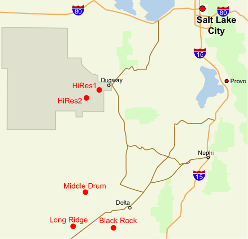
Figure 1: Map showing the location of Telescope Array relative to Salt Lake City and Dugway, Utah (the location of the High Resolution Fly’s Eye). The route from Salt Lake City to Delta is 136 miles.

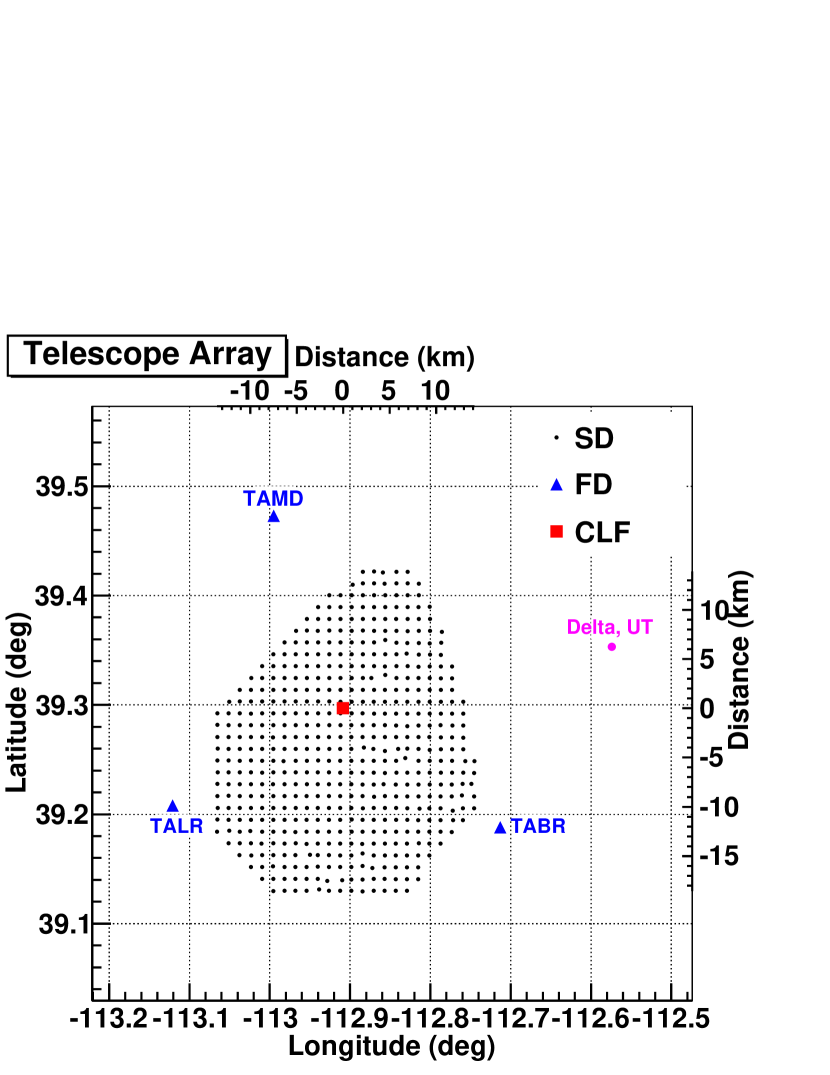
Figure 2: Map of the Telescope Array detectors. The telescope stations (Middle Drum, Long Ridge, and Black Rock Mesa) are indicated by blue triangles. The scintillator detectors are indicated by black dots and the Central Laser Facility by a red square. The ground array occupies about 700 $km^{2}$ west of Delta, Utah.

Three telescope stations view the sky over the scintillator array. The northernmost fluorescence station, known as the Middle Drum site, consists of 14 telescopes refurbished from the HiRes experiment’s HiRes-1 site. These were deployed between November, 2006 and October, 2007 and were arranged to view $\sim 120^{\circ}$ in azimuthal and $3^{\circ}-31^{\circ}$ in elevation. Compared to HiRes-1 [4], the Middle Drum site has only $1/3$ of the azimuthal coverage but observes twice the elevation, as it was deployed into two rings, each covering $14^{\circ}$ in elevation. Each telescope unit uses sample-and-hold electronics with a $5.6~{}\mu s$ gate. Each telescope camera consists of 256 PMTs covered with an ultra-violet band-pass filter. Descriptions of the Black Rock and Long Ridge telescope stations were described by Tokuno [5].

The goals of the Middle Drum spectral analysis are three-fold. The primary goal of this analysis is to determine the flux of particles using the same calibration and analysis processing tools used to produce the monocular spectrum from the HiRes-1 data. The second goal is to compare the spectra measured by the Middle Drum detector with that of HiRes-1. Since the telescope units used in both of these detectors are composed of the same equipment, the results of this comparison produce a direct link in the energy scale between these two experiments. Finally, by comparing events observed by Middle Drum and any of the other TA detectors, the energy scale of the entire Telescope Array experiment can be compared to that of the HiRes experiment. In this paper, this comparison is performed between the geometries of the events observed by Middle Drum and reconstructed using the monocular technique to those events that triggered both Middle Drum and the SD array and analyzed using a hybrid technique.

2 Event Reconstruction and Selection

The Middle Drum data and Monte Carlo events (described in section 3) were processed using the same programs created for HiRes-1 analysis [6]. The only changes made were for the location and pointing directions of the telescopes. The HiRes-1 analysis was unique in that there was limited elevation coverage and a traditional monocular reconstruction could not be performed on the data. Instead, a combined geometrical-profile reconstruction was developed by Abu-Zayyad [7] which increased the resolution of the observed showers. This technique was not required in the analysis of Middle Drum data since the detector observed longer-track events due to the increase in elevation angle coverage, however, it was used for consistency.

As at HiRes, lasers are used for light-attenuation calibration, aerosol measurements, and relative-timing variances between the three fluorescence detector sites. Most of the events observed by the Middle Drum detector belong to these calibration lasers which are primarily removed by only processing those events that are downward-tending, since the lasers are fired in either upward or horizontal directions. Some of these laser shots appear to be downward-going events due to preliminary calculations using the timing and pointing directions of the triggered tubes. These are removed using the GPS trigger time-stamp and the GPS measured site positions.

After filtering out laser events, most of those events that remain are due to electronic noise triggers, airplanes, and muons that pass through the camera’s PMTs. These are removed by determining a correlation between the time and geometrical pattern of the triggered tubes. Triggered tubes are clustered into groups of three or more tubes with difference limits on the trigger-time of $2.0~{}\mu s$ and the pointing-direction of $1.2^{\circ}$ from the previously triggered tube. These clusters are then combined into a single event-track from which a shower-detector plane (SDP) is determined. The tubes in a track are then iteratively checked and removed if greater than 3 RMS deviations away in either time or angle from the mean [6].

The Middle Drum data and Monte Carlo simulations are reconstructed in monocular mode with the geometry determined by the equation

$$t_{i}=t_{0}+\frac{R_{p}}{c}\tan\left(\frac{\pi-\psi-\chi_{i}}{2}\right),$$ (1)

where $t_{i}$ and $\chi_{i}$ are the respective trigger time and pointing direction of tube $i$, $R_{P}$ is the impact parameter of the shower with respect to the detector, $\psi$ is the angle the axis of the shower makes with respect to the direction of the core impact position around the detector, and $t_{0}$ is the time the shower is calculated to be at $R_{P}$.

The profile of the shower is calculated using the Gaisser-Hillas parameterization [8]

$$N_{e}(x)=N_{max}\times\left[\frac{x-X_{0}}{X_{max}-X_{0}}\right]^{\frac{X_{max}-X_{0}}{\lambda}}e^{\frac{X_{max}-x}{\lambda}},$$ (2)

where $N_{e}(x)$ is the number of charged particles (measured from the signal strength) at a given slant depth, $x$, in $\rm{g/cm^{2}}$; $N_{max}$ is the maximum number of secondary particles produced in the extensive air shower, located at $X_{max}$; $X_{0}$ is a fit parameter associated with the depth of the first interaction; and $\lambda$ is a fit paramater defining the width of the shower profile.

To reconstruct the Middle Drum data, as was done for HiRes-1, the time-fit was constrained by the shower profile reconstruction. This was performed by setting $\lambda$ to a constant $60~{}\rm{g/cm^{2}}$ and $X_{0}$ to a constant $-100~{}\rm{g/cm^{2}}$ in order to constrain the width and initial depth of the shower. These constants are in good agreement with average simulated shower measurements [6]. An inverse-Monte Carlo reconstruction is then made by simulating showers that closely resemble the true event using the triggered tubes. This is performed by choosing a series of $X_{max}$ values for individual Monte Carlo events over all energies in the shower library. To determine a best-fit profile reconstruction, a comparison is made between the light signal actually observed to the one simulated for each tube considered in the reconstruction. This is effective since both the timing and the profile fits are only dependent on the trigger time and pointing directions of the tubes used in the reconstruction, which determine the slant depth of the shower that each tube is observing along the axis of the shower.

Separate chi-square minimizations are then performed on the timing and the profile reconstructions for each of the constant $X_{max}$ values chosen. The timing chi-square is calculated by

$$\chi_{time}^{2}=\sum_{i}\frac{1}{\sigma_{i}^{2}}\left\{t_{i}-\left[t_{0}+\left(\frac{R_{p}}{c}\right)\tan\left(\frac{\pi-\psi-\chi_{i}}{2}\right)\right]\right\}^{2}$$ (3)

with the error, $\sigma_{i}$, determined by the time to cross the face of a PMT. The profile chi-square is calculated by

$$\chi_{profile}^{2}=\sum_{i}\left(\frac{1}{\sigma_{i}^{2}}\right)(S_{i}^{o}-S_{i}^{e})^{2}$$ (4)

where, as in the timing fit, the sum is performed over the tubes within 3 RMS deviations away from the shower-detector plane, The observed signal, $S_{i}^{o}$, is also used to calculated the uncertainty, $\sigma_{i}^{2}$, which is estimated to be $S_{i}^{o}+S$. The constant, $S=200$, is obtained through adding in quadrature the sky noise and electronic fluctuations. Details of the reconstruction codes can be found in the dissertation by Abu-Zayyad [7].

The optimal reconstruction is then determined by calculating a best combined chi-squared for each $X_{max}$ fit using

$$\chi_{comb}^{2}=\overline{\chi}_{profile}^{2}+\overline{\chi}_{time}^{2}$$ (5)

where $\overline{\chi}$ is the normalized chi-square value calculated as

$$\overline{\chi}=\chi_{fit}\times\frac{NDF_{min}}{\chi_{min}}$$ (6)

where $\chi_{fit}$ is the chi-square of from the fit for each $X_{max}$ and $NDF_{min}$ and $\chi_{min}$ are the number of degrees of freedom and the chi-square, respectively, for the smallest chi-square reconstruction. As mentioned previously, this innovative technique was developed to reconstruct HiRes-1 data which had a limited elevation coverage. Future analyses of Middle Drum data will include traditional monocular reconstruction techniques. However, this method was used in this current analysis to provide a direct comparison to the spectrum observed by HiRes-1. Additionally, this technique results in a better resolution and aperture than an unconstrained time fit, even for the longer tracks observed at the Middle Drum site.

After the selection of candidate events is obtained, quality cuts are performed on the fully reconstructed showers to remove any event that exhibits anomalous behavior. These cuts were optimized for the the short shower tracks observed by HiRes-1 [7]. The HiRes-1 analysis was ideal for cosmic rays with energy greater than $10^{18}eV$ since they could be observed from farther away and would appear as short tracks in the lower elevations. These cuts are applied to Middle Drum events since the higher-energy events would still have shorter tracks and the overlapping energy range between HiRes-1 and Middle Drum could then be directly compared. Additionally, this gives a baseline to future analyses. Events are retained if:

1. the event reconstruct well, as determined by

   • not rejecting too many off-plane tubes,

   • there are enough slant-depth bins to fit a profile,

   • a $\chi^{2}$ minimum is attained, and

   • the modified geometry still parameterizes the timing fit;

2. the angular tracks are $\geq 7.9^{\circ}$, so that there are enough triggered tubes to provide a reliable reconstruction;

3. the shower depth into the atmosphere observed by the first tube used in the reconstruction is $<1000~{}\rm{g/cm^{2}}$, so the fit is not focusing on the tail of the shower;

4. the in-plane angle, $\psi$, is $<120^{\circ}$, to make sure the detector is not overwhelmed with Čerenkov radiation; and

5. the area of the mirror observing the fitted track (away from the mirror/tube edges) is $>0.9~{}\rm{m^{2}}$, to ensure there is not a bias in the reconstructed signal strength.

3 Monte Carlo Simulation

The energy-dependent aperture of the detector is the product of the effective area and the solid angle of acceptance. This is calculated using the equations

$$(A\Omega)_{0}(\rm{m^{2}ster})=2\pi^{2}\left(R^{2}_{p~{}max}-R^{2}_{p~{}min}\right)\times\left(1-\cos\theta_{max}\right)$$ (7)

and

$$A\Omega(E)=(A\Omega)_{0}\frac{N_{recon}(E_{MC-recon})}{N_{gen}(E_{MC-gen})},$$ (8)

where $R_{P}$ is the distance of closest approach of the shower, $\theta$ is the zenith angle of the shower, $N_{recon}$ is the number of events reconstructed with energy, $E_{MC-recon}$, and $N_{gen}$ is the number of events generated with energy $E_{MC-gen}$. Counting the number of events reconstructed at an energy folds in the detector bias into the energy spectrum calculation. Alternatively, the detector efficiency at a certain energy can be calculated by replacing $N_{recon}(E_{MC-recon})$ with the number of events retained with a certain generated energy, $N_{recon}(E_{MC-gen})$. The aperture of the Middle Drum detector has been calculated to be $\sim 60\%$ that of HiRes-1 for reconstructed energies of $10^{19.0}$ eV, falling linearly to 40% at $10^{20.0}$ eV (see Figure 3).

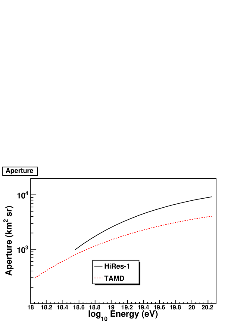
Figure 3: The calculated Middle Drum aperture compared to that for the HiRes-1 detector.

The CORSIKA-simulated shower library used by Middle Drum was the same generated for HiRes, using QGSJET01 as the hadron interaction model [4]. These showers were thrown with an isotropic distribution and consisted of $\sim 10\times$ the exposure of the Middle Drum collected data. The Monte Carlo simulated only proton events between $10^{17.5}$ eV and $10^{21.0}$ eV using values as measured by HiRes below the GZK cutoff [9] [10]. A spectral index of 3.25 was used below $10^{18.65}$ eV and 2.81 above. The spectral set was thrown without simulating the GZK suppression [11] [12]. The lower energy range was thrown out to a range of 25 km from the telescope site, well beyond where the detector is incapable of triggering on the fluorescence light of a $10^{18.65}$ eV cosmic ray shower. The higher energy range was thrown out to 50 km. The simulated showers of both energy regions were thrown with a maximum zenith angle of $80^{\circ}$. The CORSIKA output is fed into the detector Monte Caro resulting in events which look exactly like real data and are subjected to the same reconstruction programs and quality cuts.

3.1 Data-Monte Carlo Comparison

To verify the adequacy of the Monte Carlo used for the aperture calculation and to confirm that the Monte Carlo closely models the real data, it is important to compare the distributions of the reconstructed Monte Carlo events and the data. These are shown in three energy ranges ($10^{18.0-18.5}$ eV, $10^{18.5-19.0}$ eV, and $>10^{19.0}$ eV) in order to demonstrate that the Monte Carlo has the same energy evolution as the data. The variables chosen for this comparison are those that directly determine the aperture: the impact parameter, $R_{P}$ (Figure 4); the shower zenith angle, $\theta$ (Figure 5); and the shower azimuthal angle, $\phi$ (Figure 6).

The impact parameter distribution directly determines the effective area of the aperture, and, as expected, the mean of the distribution increases along with the spread, or RMS, as the energy increases. The zenith and azimuthal angles directly determine the solid angle of acceptance. For all three parameters, the (black) data points and (red) Monte Carlo histogram distributions are in excellent agreement.

It should also be noted that since the Middle Drum telescopes are pointing in the South-East direction, and that there is a quality cut removing many of those events that are pointing towards the detector, there is a depletion observed in the azimuthal distribution in this direction. This variance decreases with increasing energy since the impact parameter moves farther away from the detector and, therefore, there are fewer showers pointing above the $120^{\circ}$ limitation.

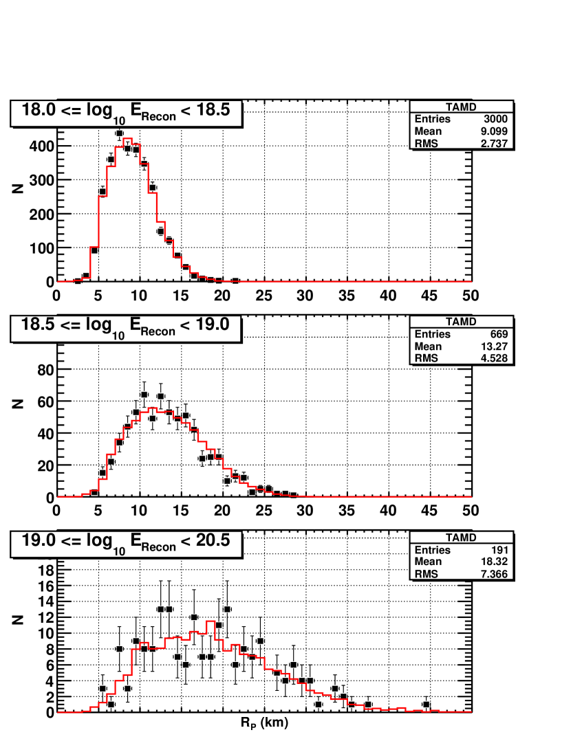
Figure 4: Comparison of the data and Monte Carlo distributions of the impact parameter, $R_{P}$, in three energy ranges: $10^{18.0-18.5}$ eV, $10^{18.5-19.0}$ eV, and $>10^{19.0}$ eV. The Monte Carlo (red histogram) is in excellent agreement with the data (black points with error bars). The number of entries indicates the number of data events observed in that energy range.

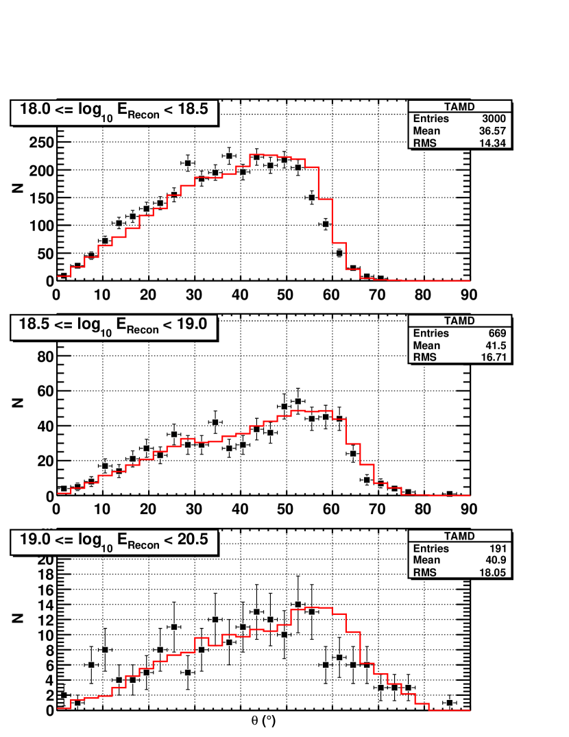
Figure 5: Comparison of the data and Monte Carlo distributions of the zenith angle, $\theta$, in three energy ranges. The Monte Carlo (red histogram) is in excellent agreement with the data (black points with error bars). The number of entries indicates the number of data events observed in that energy range.

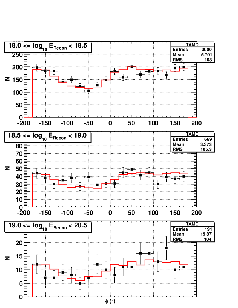
Figure 6: Comparison of the data and Monte Carlo distributions of the azimuthal angle, $\phi$, in three energy ranges: $10^{18.0-18.5}$ eV, $10^{18.5-19.0}$ eV, and $>10^{19.0}$ eV. The Monte Carlo (red histogram) is in excellent agreement with the data (black points with error bars). The number of entries indicates the number of data events observed in that energy range. The mean of this distribution indicates that most events are pointing away from the detector.

3.2 Resolution

Resolution plots indicate how well the detector simulation and reconstruction programs perform by comparing reconstructed values to generated values in Monte Carlo simulated events. The three primary parameters that show the quality of the reconstruction are the impact parameter ($R_{P}$) and the in-plane angle ($\psi$) obtained from the geometrical reconstruction, and the energy, obtained from the profile reconstruction. These are determined for the same three energy ranges as the data-Monte Carlo comparisons to show trends in the reconstruction. With increasing reconstructed energy, the geometrical parameters show a trend of improving resolution (see Figures 7 and 8). For all energy ranges, the energy resolution is on the order of 20% (see Figure 9).

Figure 7: Resolution in the measurement of the impact parameter, $R_{P}$, of Monte Carlo simulated events shown in three energy ranges: $10^{18.0-18.5}$ eV, $10^{18.5-19.0}$ eV, and $>10^{19.0}$ eV. The gaussian fit is used to determine the detector bias and resolution.

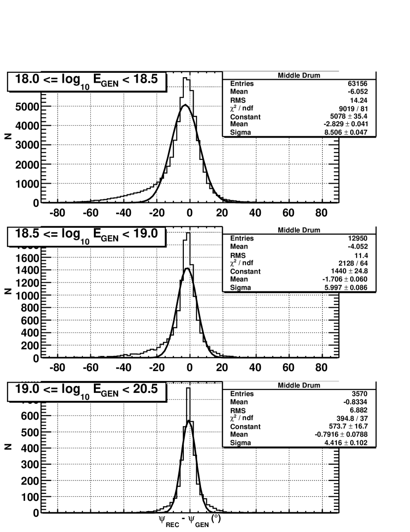
Figure 8: Resolution in the measurement of the in-plane angle, $\psi$, of Monte Carlo simulated events shown in three energy ranges: $10^{18.0-18.5}$ eV, $10^{18.5-19.0}$ eV, and $>10^{19.0}$ eV. The gaussian fit is used to determine the detector bias and resolution.

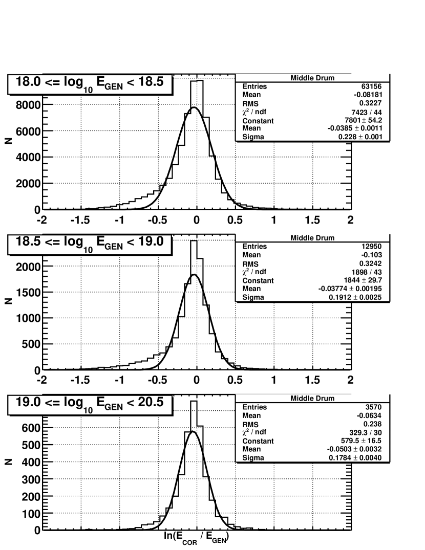
Figure 9: Resolution in the measurement of the energy of Monte Carlo simulated events shown in three energy ranges: $10^{18.0-18.5}$ eV, $10^{18.5-19.0}$ eV, and $>10^{19.0}$ eV. The gaussian fit is used to determine the detector bias and resolution.

4 The Energy Spectrum

The measured energy flux spectrum includes data collected using the Middle Drum fluorescence telescope station between December 16, 2007 and December 16, 2010 (see Figure 10). The spectrum only includes data collected on clear, moonless nights with minimal cloud cover in the view of the detector for reliable reconstruction. This amounts to $\sim 2400$ site-hours of data collection, corresponding to a 9% duty cycle. Multiplying this on-time with the aperture determines the Middle Drum exposure to be $\sim 1/3$ that of the final HiRes-1 exposure.

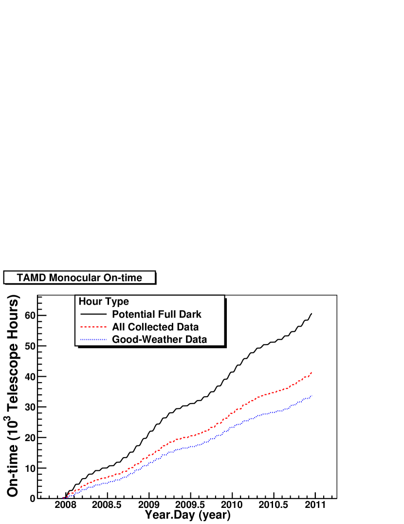
Figure 10: Integrated data collection time as a function of elapsed time for the Middle Drum fluorescence telescope site.

After three years of collecting data, 3859 events were observed. For each energy bin in which Middle Drum has observed events, the average number of events is $\sim 32.5\%$ that observed by HiRes-1. This is consistent with the Middle Drum exposure calculation. As was mentioned previously, an inverse-Monte Carlo technique is used in order to determine the energy of the shower. The Monte Carlo shower library, parameterized by the Gaisser-Hillas equation (see Equation 2), is sampled for similar $X_{max}$ values and projected along the calculated geometry. The signal for each slant-depth bin of the simulated shower is then compared to the observed shower and chi-square values are calculated for a series of $psi$ angles. The minimum chi-square value for a combined geometry and profile is determined to be the best-fit reconstruction. The showers are then distributed into tenth-decade energy bins from $10^{18.0}-10^{21.0}$ eV. The raw energy distribution for the data is shown in Figure 11.

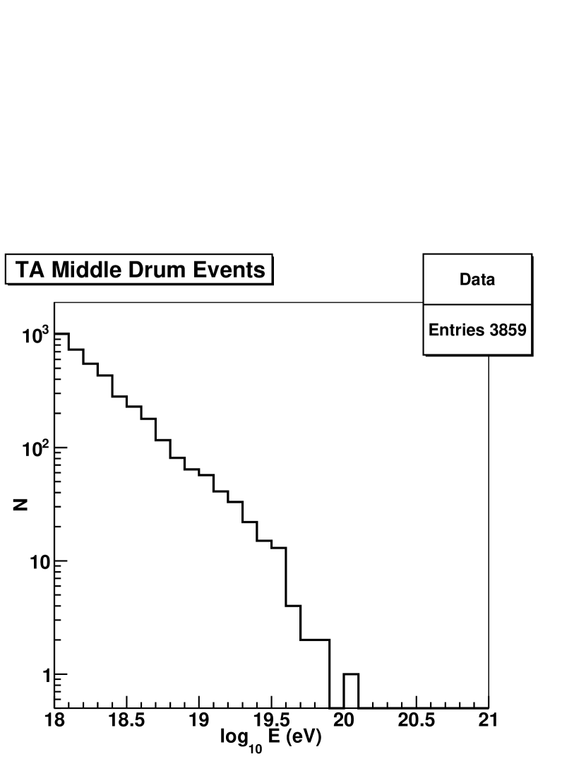
Figure 11: The raw energy distribution of events observed by the Middle Drum detector over the first three years of collection. The events are shown distributed in tenth-decade energy bins between $10^{18.0}$ eV and $10^{20.0}$ eV

The flux is calculated by combining the number of events and the exposure per energy bin using the equation

$$J(E)=\frac{n(E)}{A\Omega(E)\times\Delta t_{on}\times\Delta E},$$ (9)

where $n(E)$ is the number of events in a given energy bin, $E$; $\Delta E$ is the width of the energy bin; $A\Omega(E)$ is the energy-dependent aperture calculated from Equations 7 and 8; and $\Delta t_{on}$ is the on-time of the detector. This flux is often multiplied by the cube of the energy to flatten the spectrum in order to more clearly show the subtle features of the flux of these particles. Figure 12 shows the spectrum as determined from the Middle Drum data overlaid with that from the two HiRes detectors’ monocular reconstructions [9]. These are in excellent agreement in both normalization and shape. A consistency between the spectra measured by the Middle Drum detector and the HiRes-1 detector is determined by:

$$\Delta J=\frac{\left(J_{TAMD}-J_{HiRes-1}\right)}{\sqrt{\sigma_{TAMD}^{2}+\sigma_{HiRes-1}^{2}}}$$ (10)

where $J_{TAMD}$ and $J_{HiRes-1}$ are the measured flux and $\sigma_{TAMD}$ and $\sigma_{HiRes-1}$ are the statistical uncertainties observed by the Middle Drum and HiRes-1 detectors, respectively (see Figure 13). This calculation only included those energy bins with at least seven events observed by the Middle Drum telescopes within the HiRes-1 spectral range. This difference shows that the flux measured by Middle Drum is within $0.8\sigma$ of HiRes-1. They are consistent with the same flux level.

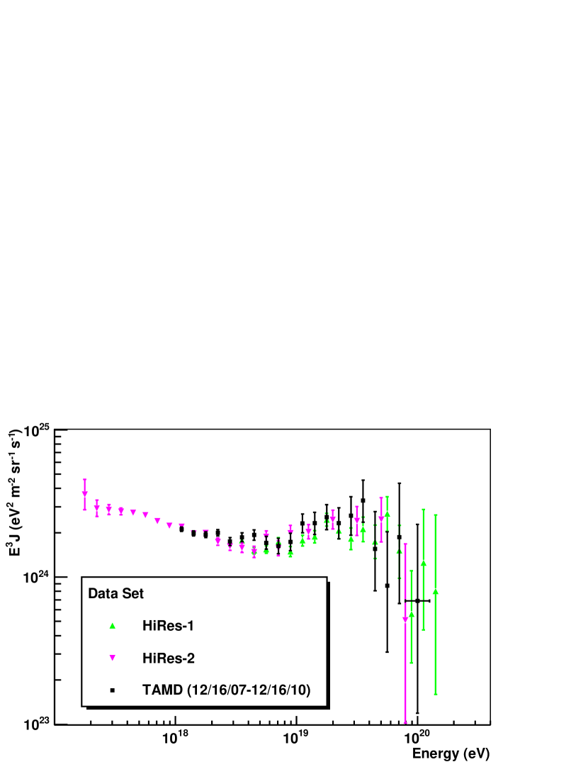
Figure 12: The energy spectra multiplied by $E^{3}$. The spectrum as determined from the Middle Drum data is shown by the black boxes. The spectra of HiRes-1 (upward, green triangles) and HiRes-2 (downward, magenta triangles) are shown for comparison. The three spectra are in excellent agreement in both normalization and shape.

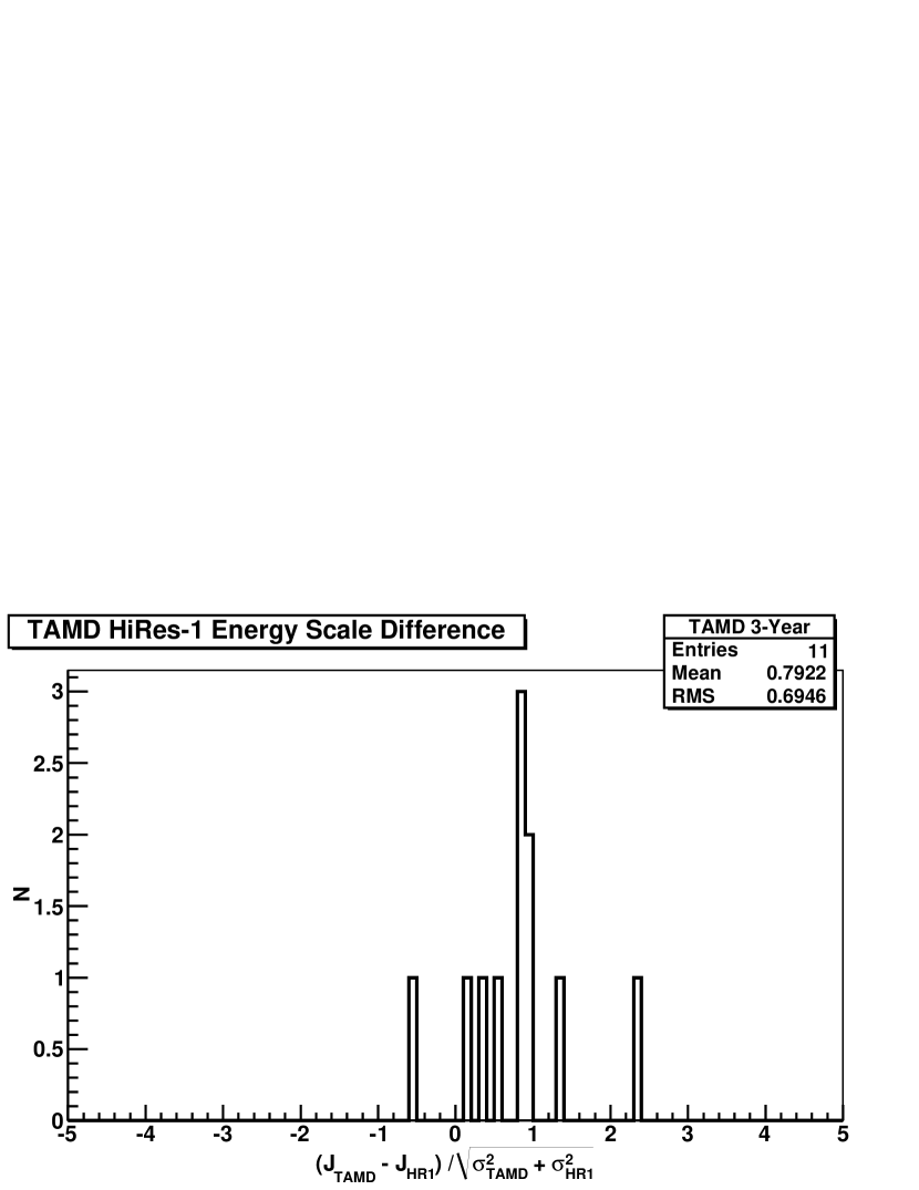
Figure 13: The bin-by-bin energy flux measurement difference between Middle Drum and HiRes-1. Only energy bins between $10^{18.55}$ and $10^{19.55}$ eV were compared since these are the only bins in the Middle Drum data where there are more than seven observed events within the HiRes-1 energy range.

Further, the Middle Drum spectrum can be quantitatively compared to the HiRes-1 spectrum by determining the $\chi^{2}$ between the flux measurements on a bin-by-bin basis. The $\chi^{2}$ value is calculated by summing over the square of each $\Delta J$ given in Equation 10. The result is a $\chi^{2}/N.D.F.=12.20/10$ for all of the overlapping bins and $\chi^{2}/N.D.F.=4.47/5$ for bins $\geq 10^{19.0}$ eV. Figure 12 shows that the $\chi^{2}$ is dominated by the difference in the measured flux in the $10^{18.65}$ eV energy bin.

Since Middle Drum measured the spectrum with the same equipment and calibration techniques and obtained the same result as HiRes-1, the HiRes-1 energy scale is thus transferred to Middle Drum. Had the energy scale changed, the rapidly falling $E^{-3}$ spectrum would have shifted by twice that increment.

5 Middle Drum Hybrid Geometry Comparison

The transfer of the energy scale from the HiRes-1 spectrum to the Middle Drum spectrum creates a direct link between the HiRes and Telescope Array experiments. The next step to completely bridge the two experiments is to determine the energy scale between those events observed by the Middle Drum detector to those that also triggered the ground array. This Middle Drum monocular-hybrid comparison will then transfer the energy scale of HiRes to the rest of Telescope Array in future studies.

The hybrid analysis begins by improving the geometrical reconstruction. Time and pulse height information of the triggered ground array scintillator detectors (SDs) are used to improve the time-versus-angle fit [13]. This is performed by calculating the SD core using the modified Linsley shower-shape [14] to obtain a lateral distribution function (LDF) which is then used to constrain the monocular time-versus-angle fit performed for the FD.

After the improved shower geometry is determined, the profile fit is performed using the inverse-Monte Carlo technique presented in this paper, however, in this fit, the geometry determined above was not adjusted to scan for a better profile fit. The hybrid data selection cuts use a combination of Middle Drum and SD information. Events are retained if:

1. the profile fit reconstructs well, as is determined in the monocular reconstruction;

2. the geometry fit has a $\chi^{2}/NDF<7$;

3. the zenith angle is $<56^{\circ}$, providing a well-reconstructed SD core impact location of simulated showers thrown up to $60^{\circ}$;

4. the SD calculated core must be within 500 meters of the SD boundary, so there is no bias in the LDF reconstruction;

5. the SD calculated core must be within 600 meters of the shower-detector plane, so the shower track remains consistent between the two detectors;

6. the angular track length is $>7.9^{\circ}$, to provide a reliable profile fit; and

7. $X_{max}$ is observed by Middle Drum, for reliable composition studies.

Since the boundary of the ground array begins $\sim 7$ km from the Middle Drum site, most of the monocular events with energy less than $10^{18.4}$ eV fall outside of the ground array (see Figures 14(a) through 14(d)). Above this energy, roughly half of the events observed monocularly have core positions within the boundary of the ground array (see Figures 15(a) and 15(b)).

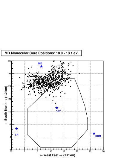
(a) $10^{18.0}-10^{18.1}$ eV

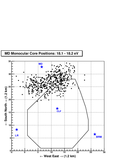
(b) $10^{18.1}-10^{18.2}$ eV

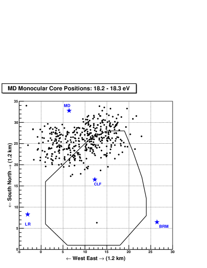
(c) $10^{18.2}-10^{18.3}$ eV

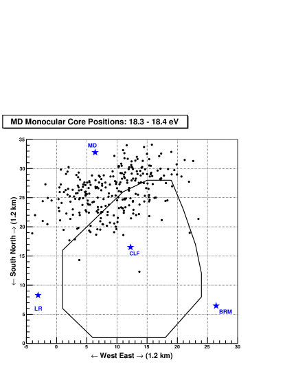
(d) $10^{18.3}-10^{18.4}$ eV

Figure 14: The core positions of the Middle Drum events observed and reconstructed in monocular mode (indicated by the points) for tenth-decade energy bins between $10^{18.0}$ and $10^{18.4}$ eV. The locations of the fluorescence stations (BRM, LR, and MD), as well as the Central Laser Facility (CLF), are indicated by stars. The perimeter of the scintillator Surface Detector (SD) array is indicated with lines. At these lowest energies, virtually all core locations are outside of the SD array.

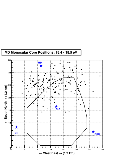
(a) $10^{18.4}-10^{18.5}$ eV

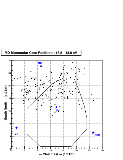
(b) $10^{18.5}-10^{18.6}$ eV

Figure 15: The core positions of the Middle Drum events observed and reconstructed in monocular mode (indicated by the points) for tenth-decade energy bins between $10^{18.4}$ and $10^{18.6}$ eV. Compared to those events shown in Figure 14, as the event energy increases, an increasing percentage of cores are observed within the SD array.

Figure 16 shows a comparison of the energy for events reconstructed from the Middle Drum data in monocular mode to the same events reconstructed in Middle Drum-hybrid mode. Only events retained in both the monocular and hybrid analyses were compared. For those events with $\sqrt{E_{mono}\times E_{hybr}}>10^{18.5}$ eV, the monocular and hybrid energies are in good agreement (see Figure 17). This provides a direct link between the events observed by Middle Drum in monocular mode to those events that also trigger the ground array. A direct comparison is thus made between HiRes and all of the Telescope Array detectors.

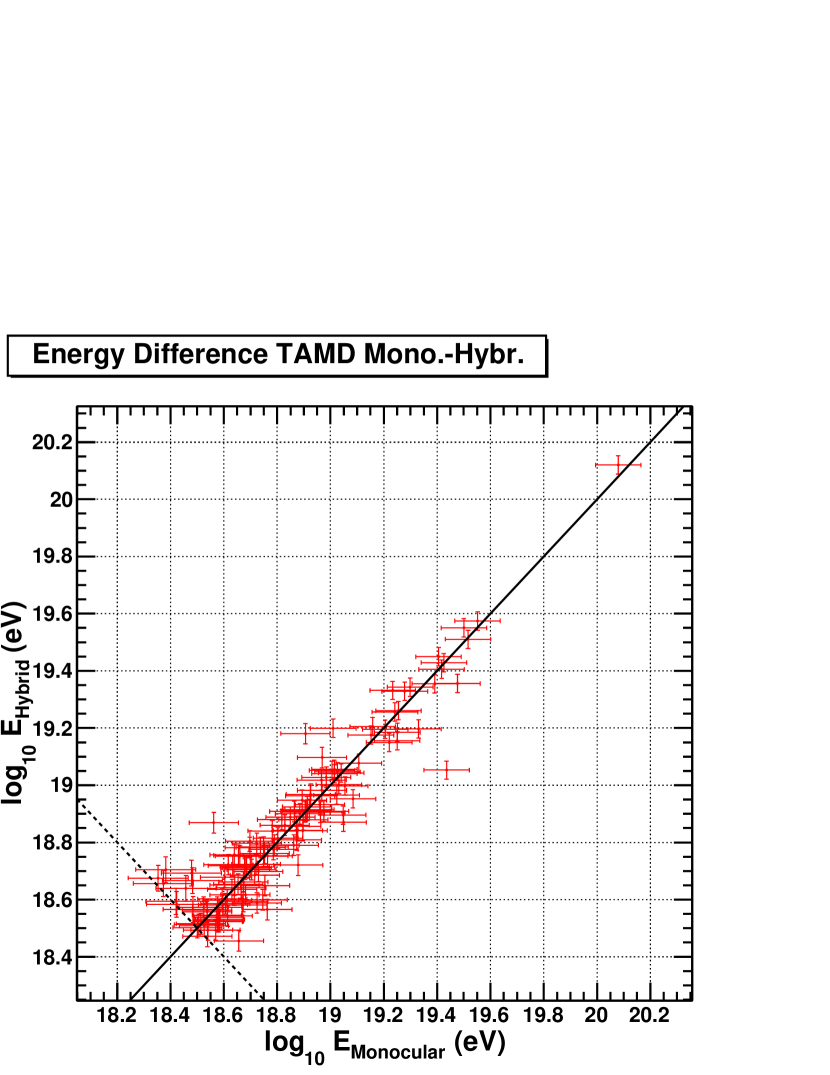
Figure 16: Comparison of event energy for cosmic ray events reconstructed in monocular mode using data collected from the Middle Drum fluorescence telescope station (abcissa) versus the energy when reconstructed in hybrid mode (ordinate) incorporating information from the scintillator surface array. The solid line drawn indicates where the two measurements would be equal. There is excellent agreement between the measurements.

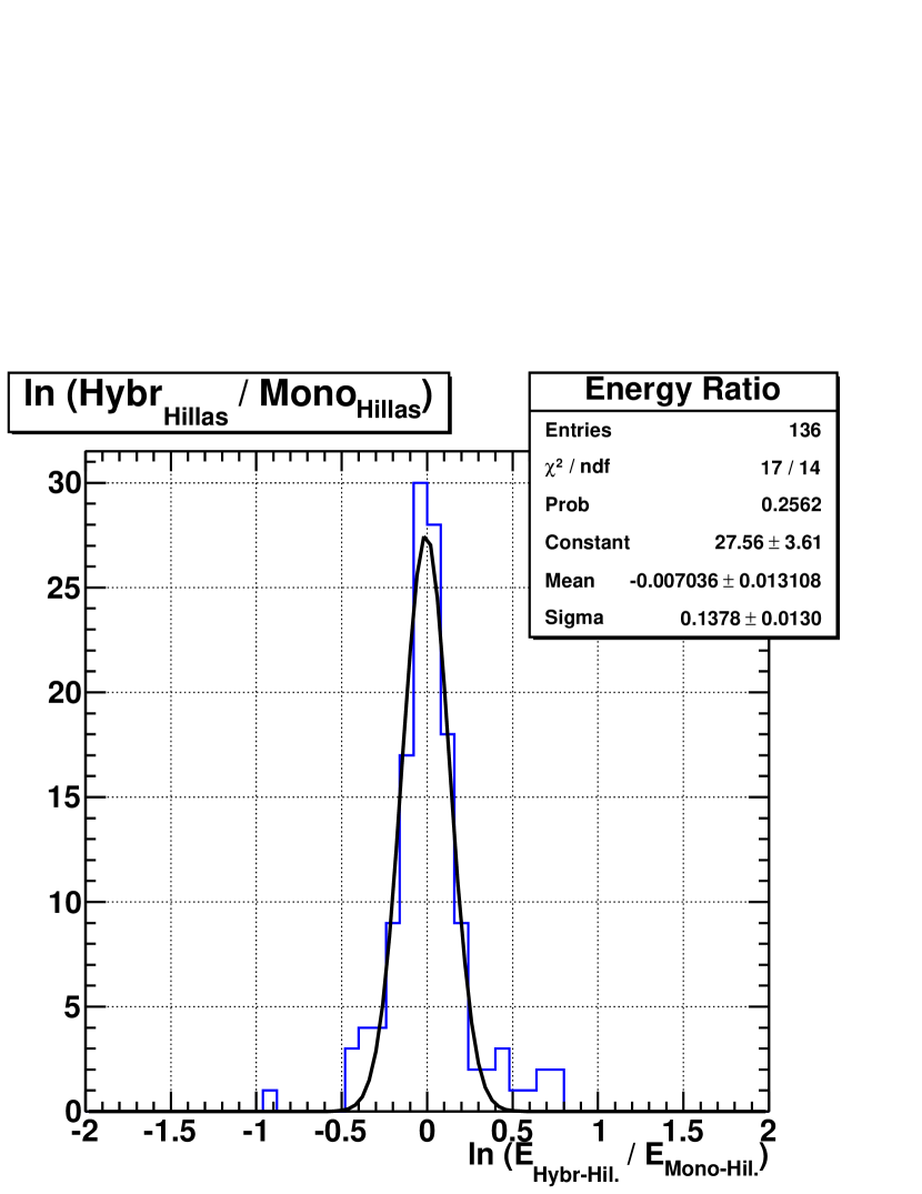
Figure 17: Spread of difference in event energy for cosmic ray events observed by the Middle Drum fluorescence telescope station reconstructed in hybrid mode incorporating information from the scintillator surface array to that reconstructed in monocular mode. The gaussian mean shows the overall difference between these reconstruction techniques, with an uncertainty indicated by the standard deviation. There is excellent agreement between the measurements.

6 Conclusions

The Telescope Array’s Middle Drum observatory uses refurbished telescopes from the High Resolution Fly’s Eye experiment. A spectral measurement was made using the first three years of the Middle Drum data collection. Both the data and simulated events were analyzed monocularly using the profile-constrained geometry reconstruction technique that was developed for the HiRes-1 data. The energy and geometrical resolutions of the Monte Carlo simulations show good agreement between what was generated and what was reconstructed and the data-Monte Carlo comparisons are in excellent agreement between simulated and real extensive air showers. The calculated Middle Drum energy spectrum is shown to be in excellent agreement with the spectra produced by the HiRes-1 monocular analysis with the difference between them less than the energy resolution of the Middle Drum reconstruction. The HiRes energy scale can now be transferred to the entire Telescope Array for further comparisons now under way.

7 Acknowledgements

The Telescope Array experiment is supported by the Japan Society for the Promotion of Science through Grants-in-Aid for Scientific Research on Specially Promoted Research (21000002) “Extreme Phenomena in the Universe Explored by Highest Energy Cosmic Rays”, and the Inter-University Research Program of the Institute for Cosmic Ray Research; by the U.S. National Science Foundation awards PHY-0307098, PHY-0601915, PHY-0703893, PHY-0758342, and PHY-0848320 (Utah) and PHY-0649681 (Rutgers); by the National Research Foundation of Korea (2006-0050031, 2007-0056005, 2007-0093860, 2010-0011378, 2010-0028071, R32-10130); by the Russian Academy of Sciences, RFBR grants 10-02-01406a and 11-02-01528a (INR), IISN project No. 4.4509.10 and Belgian Science Policy under IUAP VI/11 (ULB). The foundations of Dr. Ezekiel R. and Edna Wattis Dumke, Willard L. Eccles and the George S. and Dolores Dore Eccles all helped with generous donations. The State of Utah supported the project through its Economic Development Board, and the University of Utah through the Office of the Vice President for Research. The experimental site became available through the cooperation of the Utah School and Institutional Trust Lands Administration (SITLA), U.S. Bureau of Land Management and the U.S. Air Force. We also wish to thank the people and the officials of Millard County, Utah, for their steadfast and warm support. We gratefully acknowledge the contributions from the technical staffs of our home institutions and the University of Utah Center for High Performance Computing (CHPC).

References

- [1] T. Nonaka et al., “Calibration of TA Surface Detectors”, International Cosmic Ray Conference, 2007.
- [2] AGASA: Akeno Giant Air Shower Array,“http://www-akeno.icrr.u-tokyo.ac.jp/AGASA/”
- [3] Pierre Auger Observatory,“http://www.auger.org/”
- [4] R. U. Abbasi et al., “Measurement of the Flux of Ultrahigh Energy Cosmic Rays from Monocular Observations by the High Resolution Fly’s Eye Experiment”, Physical Review Letters (151101), 2004.
- [5] H. Tokuno et al., “On Site Calibration For New Fluorescence Detectors of the Telescope Array Experiment”, NIM-A V601, 2009, 364-371.
- [6] D. C. Rodriguez, “The Telescope Array Middle Drum Monocular Energy Spectrum and a Search For Coincident Showers Using High Resolution Fly’s Eye HiRes-1 Monocular Data”, University of Utah, Ph.D. Thesis, 2010.
- [7] T. Z. Abu-Zayyad, “The Energy Spectrum of Ultra High Energy Cosmic Rays”, University of Utah, Ph.D. Thesis, 2000.
- [8] T. K. Gaisser and A. M. Hillas, “Reliability of the Method of Constant Intensity Cuts for Reconstructing the Average Development of Vertical Showers”, International Cosmic Ray Conference, 1978.
- [9] R. U. Abbasi et al., “First Observation of the Greisen-Zatsepin-Kuzmin Suppression”, Physical Review Letters (101101), 2008.
- [10] P. Sokolsky and J. Belz and the HiRes Collaboration, “Composition of UHE Composition Measurements by Fly’s Eye, HiRes-prototype/MIA and Stereo HiRes Experiments”, International Cosmic Ray Conference, 2005.
- [11] K. Greisen, “End to the Cosmic-Ray Spectrum?”, Phys. Rev. Lett. (16), p748-750, 1966.
- [12] G. T. Zatsepin and V. A. Kuz’min, “Upper Limit of the Cosmic-Ray Spectrum”, Sov. Phys. JETP Lett. 4, p78, 1966.
- [13] M. G. Allen, “Energy Calculation of Ultra High Energy Cosmic Rays in MD Hybrid Mode with Telescope Array”, International Cosmic Ray Conference, 2011.
- [14] J. Linsley, “Thickness of the Particle Swarm in Cosmic-Ray Air Showers”, J. Phys. G: Nucl. Phys. 12 51, 1986.