Selective solvation in aqueous mixtures: Interface deformations and instability

Abstract

We briefly review the effects of selective solvation of ions in aqueous mixtures, where the ion densities and the composition fluctuations are strongly coupled. We then examine the surface tension $\gamma$ of a liquid-liquid interface in the presence of ions. We show that $\gamma$ can be decreased drastically due to the electrostatic and solvation interactions near the interface. We calculate how the free energy is changed due to small surface undulations in the presence of an electric double layer. A surface instability occurs for negative $\gamma$, which can easily be realized for antagonistic ion pairs near the solvent criticality. Three-dimensional simulation shows how the surface instability is induced.

1 Introduction

In usual electrolyte theories, ions interact via the Coulombic potential in a fluid with a homogeneous dielectric constant $\varepsilon$. However, in most of such theories, the microscopic molecular interactions between ions and solvent molecules are not explicitly considered [1, 2, 3, 4]. Around a microscopic ion such as Na⁺ or Cl^- in a polar fluid, the ion-dipole interaction gives rise to a solvation (hydration) shell composed of a number of solvent molecules (those of the more polar component for a mixture). The resultant solvation free energy per ion will be called the solvation chemical potential and will be written as $\mu_{\rm sol}^{i}$ where $i$ represents the ion species. It is important that $\mu_{\rm sol}^{i}$ strongly depends on the solvent density and/or the composition for binary mixtures, with its typical values much larger than the thermal energy $k_{B}T$. In the supercritical region of pure water the density-dependence of $\mu_{\rm sol}^{i}$ is very large. For binary mixtures [5, 6], let us introduce its derivative with respect to the composition $\phi$:

$$g_{i}=-(k_{B}T)^{-1}\partial\mu_{\rm sol}^{i}/\partial\phi,$$ (1)

which represents the degree of selective or preferential solvation of ions. Hereafter, $\phi$ is the water composition in water-oil. Then $g_{i}>0$ for hydrophilic ions and $g_{i}<0$ for hydrophobic ions. For strongly hydrophilic ions, $\mu_{\rm sol}^{i}(\phi)$ should decrease very steeply in a concentration range $0<\phi<\phi^{i}_{\rm sol}$, where hydration shells are formed [4]. Here $\phi^{i}_{\rm sol}\sim 0.002$ for Br^- in water-nitrobenzene. In this paper, we discuss the selective solvation effects in the range $\phi>\phi^{i}_{\rm sol}$ assuming the presence of well-defined hydration shells even in the water-poor region, where the variation of $\mu_{\rm sol}^{i}(\phi)$ is milder but $g_{i}$ is still large (being of order 10 for monovalent ions) [4]. Furthermore, for polyelectrolytes and colloids, dissociation of ions can occur at their ionizable groups and the degree of dissociation sensitively depends on the local composition [7, 8, 9]. Therefore, the ion densities and the solvent composition are strongly coupled ubiquitously in soft matter. Around colloids, polymers, proteins, and so on, very small heterogeneities in the solvent composition drastically alter the ion distributions and the local electric potential. As our recent findings, this selective solvation induces (i) prewetting transitions on the surfaces of ionizable rods (polyelectrolytes)[9] and spheres (colloids)[10], (ii) phase separation (precipitation) induced by a small amount of highly selective solute even outside the solvent coexistence curve [11, 12], and (iii) mesophase formation in aqueous mixtures for an antagonistic salt [2, 3, 4, 13, 14, 15].

In aqueous systems, the salt effect on the surface tension $\gamma$ has been examined extensively for an air-water interface [16, 17, 18], while it has not yet been well investigated for a liquid-liquid (oil-water) interface [19, 20]. For a small amount of solute, most experimental interpretations have been based on the Gibbs formula [22, 21] $\gamma=\gamma_{0}-k_{B}T\Gamma$, where $\gamma_{0}$ is the surface tension without solute and $\Gamma$ represents the adsorption of solute per unit area. However, we have recently shown the presence of a negative electrostatic contribution $\gamma_{\rm el}$ for a small amount of charged solute. The resultant generalized Gibbs formula is written as [4, 23, 24],

$$\gamma=\gamma_{0}-k_{B}T\Gamma+\gamma_{\rm el}.$$ (2)

Using the electric flux density $D$ and the electric field $E$, we have

$$\gamma_{\rm el} = -\int dz{\mbox{\boldmath$D$}}\cdot{\mbox{\boldmath$E$}}/8\pi$$ (3)

$$= -\int dz{\rho}{\Phi}/2,$$

where the integral is in the surface normal direction ($\parallel z$). In the second line we have used the Poisson equation $\nabla\cdot{\mbox{\boldmath$D$}}=4\pi\rho$ and the electric field expression ${\mbox{\boldmath$E$}}=-\nabla\Phi$, where $\rho$ is the charge density and $\Phi$ is the electric potential. Here, $D$, $E$, and $\rho$ are supposed to vanish far from the interface. In this paper we also assume ${\mbox{\boldmath$D$}}=\varepsilon{\mbox{\boldmath$E$}}$, where $\varepsilon$ is a dielectric constant. The electrostatic contribution is crucial for antagonistic salts [23] and ionic surfactants [24]. This result has been derived from the calculation of the excess grand potential at a planar interface. In this paper, we will calculate the excess free energy for small surface deformations, which is indeed expressed in terms of $\gamma$ in eq.(2).

In this paper, we also discuss the surface instability induced by an antagonistic salt consisting of hydrophilic and hydrophobic ions [2, 3, 4, 13, 14, 15]. An example is sodium tetraphenylborate NaBPh₄, which dissociates into hydrophilic Na⁺ with $g_{1}\gg 1$ and hydrophobic BPh${}_{4}^{-}$ with $-g_{2}\gg 1$. The latter anion consists of four phenyl rings bonded to an ionized boron. Such ion pairs behave antagonistically in aqueous mixtures in the presence of composition heterogeneity. First, they undergo microphase separation around a liquid-liquid interface on the scale of the Debye screening length. This unique ion distribution produces a large electric double layer [6, 23], leading to a large decrease in the surface tension [23] in agreement with experiments [19, 20]. From x-ray reflectivity measurements, Luo et al. [20] determined such ion distributions around a water-nitrobenzene(NB) interface by adding BPh${}_{4}^{-}$ and two species of hydrophilic ions. Second, they interact differently with water-rich and oil-rich composition fluctuations, leading to mesophases (charge density waves) near the solvent criticality. In accord with this prediction, Sadakane et al. [13] added a small amount of NaBPh₄ to a near-critical mixture of D₂O and 3-methylpyridine (3MP) to find a peak at an intermediate wave number $q_{m}$($\sim 0.1~{}$Å${}^{-1}\sim\kappa$) in the intensity of small-angle neutron scattering. The peak height was much enhanced with formation of periodic structures. (iii) Moreover, Sadakane et al. observed multi-lamellar (onion) structures at small volume fractions of 3MP (in D₂O-rich solvent) far from the criticality [14], where BPh${}_{4}^{-}$ and solvating 3MP form charged lamellae. These findings demonstrate very strong hydrophobicity of BPh${}_{4}^{-}$. (iv) Another interesting phenomenon is spontaneous emulsification (formation of small water droplets) at a water-NB interface [25, 26]. It was observed when a large pure water droplet was pushed into a cell containing NB and antagonistic salt (tetraalkylammonium chloride).

The organization of this paper is as follows. In Sec.2, we will present the background of selective solvation. In Sec.3, we will explain a Ginzburg-Landau model for electrolytes accounting for selective solvation. The surface tension formula (2) will be derived. In Sec.4, we will first calculate the free energy for a slightly deformed interface and then present simulation results on the surface instability induced by antagonistic salt.

2 Background of selective solvation

Let us suppose two species of ions ($i=1,2$) with charges $Z_{1}e$ and $Z_{2}e$ ($Z_{1}>0$, $Z_{2}<0$). At low ion densities, the total ion chemical potentials $\mu_{i}$ in a mixture solvent are expressed as

$$\mu_{i}=k_{B}T\ln(n_{i}\lambda_{i}^{3})+Z_{i}e\Phi+\mu_{\rm sol}^{i}(\phi),$$ (4)

where $\phi$ is the water composition and $\lambda_{i}$ is the thermal de Broglie length (but is an irrelevant constant in the isothermal condition) and $\Phi$ is the local electric potential. For neutral hydrophobic particles the electrostatic term is nonexistent. The $\mu_{i}$ is a constant in equilibrium except for the interface region. We consider a liquid-liquid interface between a polar (water-rich) phase $\alpha$ and a less polar (oil-rich) phase $\beta$ with bulk compositions $\phi_{\alpha}$ and $\phi_{\beta}$ with $\phi_{\alpha}>\phi_{\beta}$. Thus $\mu_{\rm sol}^{i}(\phi)$ takes different bulk values in the two phases due to its composition dependence. So we define

$$\Delta\mu_{\alpha\beta}^{i}=\mu_{\rm sol}^{i}(\phi_{\beta})-\mu_{\rm sol}^{i}(\phi_{\alpha}),$$ (5)

which is called the Gibbs transfer free energy (per ion here) in electrochemistry [4, 27, 28, 29, 30, 31]. The bulk ion densities far from the interface are written as $n_{i\alpha}$ in phase $\alpha$ and $n_{i\beta}$ in phase $\beta$. From the charge neutrality condition in the bulk regions, we require $Z_{1}n_{1\alpha}+Z_{2}n_{2\alpha}=0$ and $Z_{1}n_{1\beta}+Z_{2}n_{2\beta}=0.$ The potential $\Phi$ tends to constants $\Phi_{\alpha}$ and $\Phi_{\beta}$ in the bulk two phases, yielding a Galvani potential difference,

$$\Delta\Phi=\Phi_{\alpha}-\Phi_{\beta},$$ (6)

across the interface. Here $\Phi$ approaches its limits on the scale of the Debye screening lengths, $\kappa_{\alpha}^{-1}$ and $\kappa_{\beta}^{-1}$, away from the interface, so we assume that the system extends longer than $\kappa_{\alpha}^{-1}$ in phase $\alpha$ and $\kappa_{\beta}^{-1}$ in phase $\beta$. For air-water interfaces, there are no ions in the air region, so $\kappa_{\beta}=0$, however. The continuity of $\mu_{i}$ across the interface gives

$$k_{B}T\ln(n_{i\alpha}/n_{i\beta})+Z_{i}e\Delta\Phi-\Delta\mu_{\alpha\beta}^{i}=0,$$ (7)

where $i=1,2$. After some calculations, $\Delta\Phi$ is expressed as [27, 6]

$$\Delta\Phi=[{\Delta\mu_{\alpha\beta}^{1}-\Delta\mu_{\alpha\beta}^{2}}]/{e(Z_{1}+|Z_{2}|)}.$$ (8)

Similar potential differences also appear at liquid-solid interfaces (electrodes) [31]. The ion densities in the bulk two phases (in the dilute limit) are simply related by

$$\frac{n_{1\beta}}{n_{1\alpha}}=\frac{n_{2\beta}}{n_{2\alpha}}=\exp\bigg{[}-\frac{|Z_{2}|{\Delta\mu_{\alpha\beta}^{1}}+Z_{1}\Delta\mu_{\alpha\beta}^{2}}{(Z_{1}+|Z_{2}|)k_{B}T}\bigg{]}.$$ (9)

However, if three ion species are present, the ion partitioning between two phases is much more complicated [23].

The Gibbs transfer free energy has been determined at present for water-nitrobenzene (NB) [27, 28, 29, 30] and water-1,2-dichloroethane(EDC) [29] at room temperatures, where the dielectric constant of NB ($\sim 35$) is larger than that of EDC ($\sim 10$). In the case of water-NB, the ratio $\Delta\mu_{\alpha\beta}^{i}/k_{B}T$ is $13.6$ for Na⁺, $27.1$ for Ca²⁺, and $11.3$ for Br^- as examples of hydrophilic ions, while it is $-14.4$ for hydrophobic BPh${}_{4}^{-}$. In the case of water-EDC, it is $22.7$ for Na⁺ and $17.5$ for Br^-, while it is $-14.1$ for BPh${}_{4}^{-}$. The amplitude $|\Delta\mu_{\alpha\beta}^{i}|/k_{B}T$ for hydrophilic ions is larger for EDC than for NB and is very large for multivalent ions. For H⁺ (more precisely hydronium ions H₃O⁺), $\Delta\mu_{\alpha\beta}^{i}$ assumes positive values close to those for Na⁺ in these two mixtures.

3 Ginzburg-Landau theory of mixture electrolytes

3.1 Ginzburg-Landau free energy

We consider a Ginzburg-Landau free energy $F$ for a polar binary mixture (water-oil) containing a small amount of a monovalent salt ($Z_{1}=1$, $Z_{2}=-1$). The ions are dilute and their volume fractions are negligible. The variables $\phi$, $n_{1}$, and $n_{2}$ are coarse-grained ones varying smoothly on the molecular scale. We also neglect the image interaction [17], though it was included in our previous papers [6, 23]. See our previous analysis [6] for relative importance between the image interaction and the solvation interaction at a liquid-liquid interface. The $F$ is the following space integral in the cell,

$$F=\int d{\mbox{\boldmath$r$}}\bigg{[}f_{\rm tot}+\frac{1}{2}C|\nabla\phi|^{2}+\frac{\varepsilon}{8\pi}{\mbox{\boldmath$E$}}^{2}\bigg{]}.$$ (10)

The first term $f_{\rm tot}$ depends on $\phi$, $n_{1}$, and $n_{2}$ as

$${f_{\rm tot}}=f(\phi)+k_{B}T\sum_{i}n_{i}\bigg{[}\ln(n_{i}\lambda_{i}^{3})-1-g_{i}\phi\bigg{]}.$$ (11)

If the solvent molecular volumes of the two components take a common value $v_{0}=a^{3}$ with $a\sim 3{\rm\AA}$, we may assume the Bragg-Williams form [22, 32] for the first term,

$$\frac{v_{0}f}{k_{B}T}=\phi\ln\phi+(1-\phi)\ln(1-\phi)+\chi\phi(1-\phi),$$ (12)

where $\chi$ is the interaction parameter dependent on $T$. The critical value of $\chi$ is 2 without ions. The $\lambda_{i}=\hbar(2\pi/m_{i}k_{B}T)^{1/2}$ in eq.(11) is the thermal de Broglie wavelength of the species $i$ with $m_{i}$ being the molecular mass. The $g_{1}$ and $g_{2}$ are the solvation coupling constants assumed to be constants. The coefficient $C$ in the gradient part of eq.(10) is of order $k_{B}T/a$ and should be determined from the surface tension data or from the scattering data. The electric field is written as ${\mbox{\boldmath$E$}}=-\nabla\Phi$. The electric potential $\Phi$ satisfies the Poisson equation,

$$-\nabla\cdot\varepsilon\nabla\Phi=4\pi\rho.$$ (13)

For simplicity, the dielectric constant $\varepsilon$ is assumed to depend on $\phi$ as

$$\varepsilon(\phi)=\varepsilon_{0}+\varepsilon_{1}\phi.$$ (14)

where $\varepsilon_{0}$ and $\varepsilon_{1}$ are positive constants. A linear composition dependence of $\varepsilon(\phi)$ was observed by Debye and Kleboth for a mixture of nitrobenzene-2,2,4-trimethylpentane [33].

The solvation terms ($\propto g_{i}$) follow if $\mu_{\rm sol}^{i}(\phi)$ ($i=1,2$) depend on $\phi$ linearly as

$$\mu_{\rm sol}^{i}(\phi)=A_{i}-k_{B}Tg_{i}\phi,$$ (15)

where $g_{i}$ are constants independent of $\phi$. We assume the presence of well-defined solvation shells in the concentarion range $\phi>\phi_{\rm sol}^{i}$ for hydrophilic ions (see the sentences below eq.(1)). The first term $A_{i}$ is a constant yielding a contribution linear with respect to $n_{i}$ in $f_{\rm tot}$, so it is irrelevant at constant ion numbers. The difference of the solvation chemical potentials in two-phase coexistence in eq.(5) is given by $\Delta\mu_{\rm sol}^{i}(\phi)=k_{B}Tg_{i}\Delta\phi,$ where $\Delta\phi=\phi_{\alpha}-\phi_{\beta}$ is the composition difference. From eqs.(7) and (8), the Galvani potential difference and the ion reduction factor are expressed in terms of $g_{i}\Delta\phi$ as

$$\Delta\Phi=k_{B}T(g_{1}-g_{2})\Delta\phi/2e,$$ (16)

$${n_{1\beta}}/{n_{1\alpha}}={n_{2\beta}}/{n_{2\alpha}}=\exp[-(g_{1}+g_{2}){\Delta\phi}/{2}].$$ (17)

The equilibrium interface profiles can be calculated by requiring the homogeneity of the chemical potentials $h=\delta F/\delta\phi$ and $\mu_{i}=\delta F/\delta n_{i}$. Some calculations give

$$h=f^{\prime}-C\nabla^{2}\phi-\frac{\varepsilon_{1}}{8\pi}{\mbox{\boldmath$E$}}^{2}-k_{B}T\sum_{i}g_{i}n_{i},$$ (18)

$$\mu_{i}=k_{B}T[\ln(n_{i}\lambda_{i}^{3})-g_{i}\phi]+Z_{i}e\Phi,$$ (19)

where $f^{\prime}=\partial f/\partial\phi$. The ion distributions are expressed in terms of $\phi$ and $\Phi$ in the modified Poisson-Boltzmann relations [6],

$$n_{i}=n_{i}^{0}\exp[g_{i}\phi-Z_{i}e\Phi/k_{B}T].$$ (20)

The coefficients $n_{i}^{0}$ are determined from the conservation of the ion numbers, $\langle{n_{i}}\rangle=V^{-1}\int d{\mbox{\boldmath$r$}}n_{i}({\mbox{\boldmath$r$}})=n_{0},$ where $\langle{\cdots}\rangle=V^{-1}\int d{\mbox{\boldmath$r$}}(\cdots)$ denotes the space average with $V$ being the cell volume. The average $n_{0}=\langle{n_{1}}\rangle=\langle{n_{2}}\rangle$ is a given constant density.

3.2 Interface profiles and surface tension

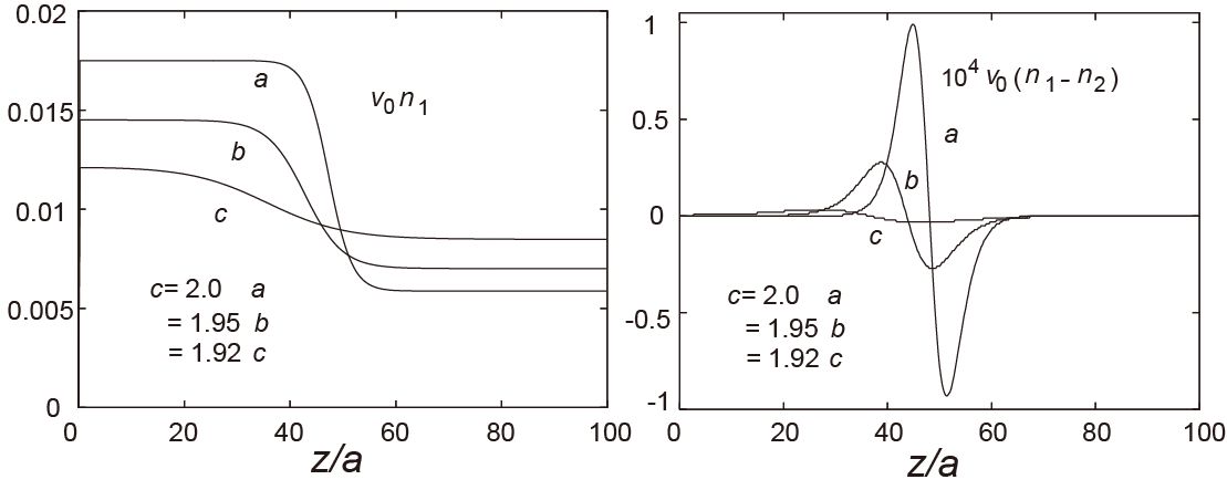
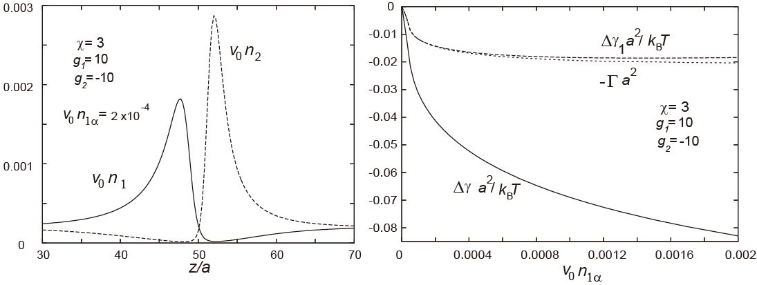
First, we give typical examples of the interface profiles for $\varepsilon_{1}/\varepsilon_{0}=4/3$ and $e^{2}/\varepsilon_{1}k_{B}T=20/\pi$. In Fig. 1, we display the ion density $n_{1}(z)$ and the density difference $n_{1}(z)-n_{2}(z)$ proportional to the charge density for hydrophilic ion pairs with $g_{1}=4$ and $g_{2}=2$. We use the free energy density in eq.(12) and set $\chi=2,1.95$, and 1.92. Note that the critical value of $\chi$ is shifted as $\chi_{c}=2+(g_{1}+g_{2})^{2}v_{0}n_{0}/2$ in the presence of ions in the mean-field theory. As $\chi\to\chi_{c}$, the electric double layer at the interface diminishes. On the other hand, the ion distributions for a pair of strongly hydrophilic and hydrophobic ions are very singular. In the left panel of Fig.2, we show the ion densities for antagonistic ion pairs with $g_{1}=-g_{2}=10$, where $\chi=3$ and $v_{0}n_{1\alpha}=v_{0}n_{1\beta}=2\times 10^{-4}$. For this hydrophilic and hydrophobic ion pair, a microphase separation forming a large electric double layer is apparent.

Figure 1: Normalized ion density $v_{0}n_{1}(z)$ (left) and normalized charge density $v_{0}(n_{1}(z)-n_{2}(z))$ (multiplied by $10^{4}$) (right) with $g_{1}=4$ and $g_{2}=2$ for $\chi=2$ in (a), $1.95$ in (b), and 1.92 in (c).

Figure 2: Left: Normalized ion densities, where $\chi=3$, $g_{1}=-g_{2}=10$, and $v_{0}n_{1\alpha}=v_{0}n_{1\beta}=2\times 10^{-4}$. For this hydrophilic and hydrophobic ion pair, a microphase separation forming a large electric double layer is apparent. Right: $a^{2}\Delta\gamma/k_{B}T$ and $a^{2}\Delta\gamma_{1}/k_{B}T$ as functions of $v_{0}n_{1\alpha}$, where $\gamma_{1}$ is the first term in eq.(24) and $\Delta\gamma_{1}=\gamma_{1}-\gamma_{0}$ is very close to $-\Gamma a^{2}$. This shows that the electrostatic part $\gamma_{\rm e}=\gamma-\gamma_{1}=-\int dz\varepsilon E^{2}/8\pi$ dominates over $\Delta\gamma_{1}\cong-k_{B}T\Gamma$.

Next, we consider the surface tension of a liquid-liquid interface in our Ginzburg-Landau scheme, where all the quantities depend on $z$. In equilibrium we minimize the grand potential $\Omega=\int d{z}\omega$, where the grand potential density $\omega$ is written as

$$\omega=f_{\rm tot}+\frac{C}{2}\phi^{\prime 2}+\frac{\varepsilon}{8\pi}{\mbox{\boldmath$E$}}^{2}-h\phi-\mu_{1}n_{1}-\mu_{2}n_{2}.$$ (21)

Using eqs.(17) and (18) we find $d(\omega+\rho\Phi)/dz=2C\phi^{\prime}\phi^{\prime\prime}$. Hereafter $\phi^{\prime}=d\phi/dz$ and $\phi^{\prime\prime}=d^{2}\phi/dz^{2}$. Thus $\omega(z)$ tends to a common constant $\omega_{\infty}$ as $z\to\pm\infty$ and

$$\omega=C\phi^{\prime 2}-\rho\Phi+\omega_{\infty}.$$ (22)

The surface tension $\gamma=\int dz[\omega(z)-\omega_{\infty}]$ is then written as [6, 23]

$$\gamma=\int dz\bigg{[}C\phi^{\prime 2}-\frac{\varepsilon}{4\pi}{\mbox{\boldmath$E$}}^{2}\bigg{]}.$$ (23)

From eq.(20) we may also devise the following formula,

$$\gamma=\int dz\bigg{[}f(\phi)+\frac{C}{2}\phi^{\prime 2}-k_{B}Tn-h\phi-C_{\alpha}\bigg{]}-\int dz\frac{\varepsilon}{8\pi}{\mbox{\boldmath$E$}}^{2},$$ (24)

where $C_{\alpha}=f(\phi_{\alpha})-k_{B}Tn_{\alpha}-h\phi_{\alpha}$ and $h=[f(\phi_{\alpha})-f(\phi_{\beta})-k_{B}T(n_{\alpha}-n_{\beta})]/\Delta\phi$ with $n_{\alpha}$ and $n_{\beta}$ being the bulk values of $n=n_{1}+n_{2}$. In accord with eq.(2), the right hand side of eq.(24) may be expanded for small $n_{0}$ as

$$\gamma=\gamma_{0}-k_{B}T\Gamma-\int dz\frac{\varepsilon}{8\pi}{\mbox{\boldmath$E$}}^{2}+\cdots,$$ (25)

where $\gamma_{0}$ is the surface tension for $n_{0}=0$. In the second term, $\Gamma$ is the preferential adsorption at the interface expressed as

$$\Gamma=\int dz\bigg{[}n-n_{\alpha}-\frac{\Delta n}{\Delta\phi}(\phi-\phi_{\alpha})\bigg{]},$$ (26)

where $\Delta n=n_{\alpha}-n_{\beta}$. Thus the second term is the solute correction in the Gibbs formula. The third term is the electrostatic contribution growing for antagonistic salt[23, 2] and ionic surfactant [24]. Thus eq.(25) is the generalized Gibbs formula including the electrostatic part. In the right panel of Fig.2, we examine how $\Delta\gamma=\gamma-\gamma_{0}$ and $\Delta\gamma_{1}=\gamma_{1}-\gamma_{0}$ are decreased with increasing $n_{1\alpha}$ for $g_{1}=-g_{2}=10$, where $\gamma_{1}$ is the first term on the right hand side of eq.(24). We notice the following. (i) The changes $\Delta\gamma$ and $\Delta\gamma_{1}$ are both proportional to $n_{1\alpha}^{1/2}$ at small $v_{0}n_{1\alpha}$. Here $|\Delta\gamma|/(v_{0}n_{1\alpha})^{1/2}$ is of order unity, so $\Delta\gamma$ is appreciable even for very small $v_{0}n_{1\alpha}$. This salt-density dependence was observed for a water-air interface [16, 23]. (ii) The electrostatic part $\gamma_{\rm e}\equiv-\int dz\varepsilon E^{2}/8\pi$ is known to be important in this case from comparison between $\Delta\gamma_{1}$ and $\Delta\gamma=\Delta\gamma_{1}+\gamma_{\rm e}$. (iii) We confirm that the modified Gibbs relation $\Delta\gamma_{1}\cong-k_{B}T\Gamma$ holds excellently.

4 Interface deformations

4.1 Free energy change

We examine how the free energy changes for small deformations of the interface position $z=\zeta(x,y)$. To this end, we superimpose small deviations $\delta\phi$ and $\delta n_{i}$ on the equilibrium interface profiles, $\phi=\phi(z)$ and $n_{i}=n_{i}(z)$, respectively. For simplicity, we replace $\phi(z)$ and $n_{i}(z)$ by $\phi(z-\zeta)$ and $n_{i}(z-\zeta)$, respectively. For small $\zeta$. we set

$$\delta\phi=-\phi^{\prime}(z)\zeta,\quad\delta n_{i}=-n_{i}^{\prime}(z)\zeta,$$ (27)

where $\phi^{\prime}=d\phi/dz$ and $n_{i}^{\prime}=dn_{i}/dz$, Then the deviation of the dielectric constant $\delta\varepsilon=-\varepsilon_{1}\phi^{\prime}\zeta$ and that of the charge density $\delta\rho=-\rho^{\prime}\delta\zeta$ are linear in $\zeta$, where $\rho^{\prime}=e(n_{1}^{\prime}-n_{2}^{\prime})$. However, the electric potential is the solution of the Poisson equation (12) and its deviation is expanded as $\Phi_{1}+\Phi_{2}+O(\zeta^{3})$ up to order $\zeta^{2}$, where $\Phi_{1}\sim\zeta$ and $\Phi_{2}\sim\zeta^{2}$. To first and second orders in $\zeta$, eq.(13) yields

$$\nabla\cdot[\delta\varepsilon\nabla\Phi+\varepsilon\nabla\Phi_{1}]=4\pi\rho^{\prime}\zeta,$$ (28)

$$\nabla\cdot[\delta\varepsilon\nabla\Phi_{1}+\varepsilon\nabla\Phi_{2}]=0.$$ (29)

Hereafter $\Phi=\Phi(z)$ denotes the unpertubed potential for $\zeta=0$. The second-order change in the electrostatic free energy $F_{e}=\int d{\mbox{\boldmath$r$}}\varepsilon{\mbox{\boldmath$E$}}^{2}/8\pi$ is written as

$$\delta F_{e} = \int d{\mbox{\boldmath$r$}}\bigg{[}\frac{\varepsilon}{8\pi}|{\nabla\Phi_{1}}|^{2}+\frac{\Phi^{\prime}}{4\pi}\bigg{(}\delta\varepsilon\frac{\partial\Phi_{1}}{\partial z}+\varepsilon\frac{\partial\Phi_{2}}{\partial z}\bigg{)}\bigg{]}$$ (30)

$$= \int d{\mbox{\boldmath$r$}}{\varepsilon}|{\nabla\Phi_{1}}|^{2}/{8\pi}.$$

If we multiply eq.(29) by $\Phi$ and integrate over space, we find $\int d{\mbox{\boldmath$r$}}{\Phi^{\prime}}(\delta\varepsilon{\partial\Phi_{1}}/{\partial z}+\varepsilon{\partial\Phi_{2}}/{\partial z})=0$. Thus, in eq.(30), the second line follows from the first line. Furthermore, taking the derivative of eq.(18) with respect to $z$ gives $f^{\prime\prime}\phi^{\prime}-C\phi^{\prime\prime\prime}-\varepsilon_{1}\Phi^{\prime}\Phi^{\prime\prime}/4\pi-k_{B}T\sum_{i}g_{i}n_{i}^{\prime}=0$, where $f^{\prime\prime}=\partial^{2}f/\partial\phi^{2}$, $\phi^{\prime\prime\prime}=\partial^{3}\phi/\partial z^{3}$, $\Phi^{\prime}=d\Phi/dz$, and $\Phi^{\prime\prime}=d^{2}\Phi/dz^{2}$. We also find the relation $\sum_{i}(\delta n_{i})^{2}/n_{i}=\sum_{i}g_{i}\delta n_{i}\delta\phi+\delta\rho\Phi^{\prime}\zeta$ from eq.(20). Using these relations, we calculate the second-order deviation of the free energy change $F$ as

$$\delta F=\int d{\mbox{\boldmath$r$}}\bigg{[}\frac{C}{2}\phi^{\prime 2}|\nabla_{\perp}\zeta|^{2}+\frac{\varepsilon}{8\pi}\nabla\Phi_{1}\cdot\nabla\varphi\bigg{]},$$ (31)

where $\nabla_{\perp}=(\partial/\partial x,\partial/\partial y)$ and we introduce the combination $\varphi=\Phi_{1}+\zeta\Phi^{\prime}$ linear in $\zeta$. From eq.(28) $\varphi$ is related to $\zeta$ by

$$\nabla\cdot\varepsilon\nabla\varphi=\varepsilon\Phi^{\prime}\nabla_{\perp}^{2}\zeta,$$ (32)

so $\varphi=0$ for homogeneous $\zeta$. Using the surface tension expression in eq.(23), we obtain

$$\delta F=\int d{\mbox{\boldmath$r$}}_{\perp}\frac{\gamma}{2}|\nabla_{\perp}\zeta|^{2}+\int d{\mbox{\boldmath$r$}}\frac{\varepsilon}{8\pi}|\nabla\varphi|^{2},$$ (33)

where $d{\mbox{\boldmath$r$}}_{\perp}=dxdy$ in the first term is the integral in the $xy$ plane. For homogeneous $\zeta$, we have $\delta F=0$ since the deviations (26) represent a uniform translation of the interface.

Let us consider the two-dimensional Fourier transform $\zeta_{\mbox{\boldmath$k$}}=\int d{\mbox{\boldmath$r$}}_{\perp}e^{-i{\mbox{\boldmath$k$}}\cdot{\mbox{\boldmath$r$}}_{\perp}}\zeta({\mbox{\boldmath$r$}}_{\perp})$, where ${\mbox{\boldmath$k$}}=(k_{x},k_{y})$ is the lateral wave vector. Then eq.(33) is rewritten as

$$\delta F=\frac{1}{2}\int\frac{d{\mbox{\boldmath$k$}}}{(2\pi)^{2}}({\gamma}k^{2}+\Delta_{k}k^{2})|{\zeta}_{\mbox{\boldmath$k$}}|^{2}$$ (34)

where $\Delta_{k}k^{2}$ arises from the second term in eq.(33). To calculate $\Delta_{k}$ the Fourier transform $\varphi_{\mbox{\boldmath$k$}}(z)=\int d{\mbox{\boldmath$r$}}_{\perp}e^{-i{\mbox{\boldmath$k$}}\cdot{\mbox{\boldmath$r$}}_{\perp}}\varphi({\mbox{\boldmath$r$}}_{\perp},z)$ is introduced. From eq.(32) we may set $\varphi_{\mbox{\boldmath$k$}}(z)=-k^{2}G_{k}(z)\zeta_{\mbox{\boldmath$k$}}$, where $G_{k}(z)$ is a function of $z$ satisfying

$$(\nabla_{z}\varepsilon\nabla_{z}-\varepsilon k^{2})G_{k}=\varepsilon\Phi^{\prime}.$$ (35)

In terms of $G_{k}$, $\Delta_{k}$ is expressed as

$$\Delta_{k}=-k^{2}\int dz~{}\varepsilon(z)\Phi^{\prime}(z)G_{k}(z)/4\pi.$$ (36)

In particular, we consider the long wavelength limit with $k=|{\mbox{\boldmath$k$}}|\ll\xi^{-1},\kappa_{\alpha}$, and $\kappa_{\beta}$, where $\xi$ is the interface thickness and $\kappa_{\alpha}$ and $\kappa_{\beta}$ are the Debye wave numbers in the bulk two phases. In the monovalent case they are given by

$$\kappa_{\alpha}=(8\pi n_{\alpha}e^{2}/\varepsilon_{\alpha}k_{B}T)^{1/2},$$

$$\kappa_{\beta}=(8\pi n_{\beta}e^{2}/\varepsilon_{\beta}k_{B}T)^{1/2},$$ (37)

where $\varepsilon_{\alpha}$ and $\varepsilon_{\beta}$ are the dielectric constants in the two phases. In this case, for $|z|$ larger than $\xi,\kappa_{\alpha}^{-1}$, and $\kappa_{\beta}^{-1}$, we have $G_{k}(z)=W_{0}e^{-k|z|}/(\varepsilon_{\alpha}+\varepsilon_{\beta})k$, where

$$W_{0}=-\int dz~{}\varepsilon\Phi^{\prime}.$$ (38)

Thus $\Delta_{k}$ is proportional to $k$ as

$$\Delta_{k}=W_{0}^{2}k/4\pi(\varepsilon_{\alpha}+\varepsilon_{\beta}).$$ (39)

If $\xi$ is shorter than $\kappa_{\alpha}^{-1}$ and $\kappa_{\beta}^{-1}$, the potential $\Phi(z)$ may be calculated from the nonlinear Poisson-Boltzmann equation[23], leading to

$$W_{0}=\varepsilon_{\beta}\Delta\Phi+\frac{k_{B}T}{e}(\varepsilon_{\alpha}-\varepsilon_{\beta})\ln\bigg{[}\frac{1+be^{\Delta U/2}}{1+be^{-\Delta U/2}}\bigg{]},$$ (40)

where $b=\varepsilon_{\beta}\kappa_{\beta}/\varepsilon_{\alpha}\kappa_{\alpha}$ and $\Delta U=e\Delta\Phi/k_{B}T$. If $\Delta U$ is small, we have $W_{0}\cong(1+b)^{-1}(\varepsilon_{\beta}+b\varepsilon_{\alpha})\Delta\Phi$, which simply follows from the Debye-H$\ddot{\rm u}$ckel approximation. In the simple case $\varepsilon_{\alpha}=\varepsilon_{\beta}$, we have $W_{0}=\varepsilon_{\beta}\Delta\Phi$ and $\Delta_{k}=k_{B}T(\Delta U)^{2}\ell_{B}^{-1}k^{3}/4\pi$, where $\ell_{B}=e^{2}/\varepsilon_{\alpha}k_{B}T$ is the Bjerrum length common in the two phases.

4.2 Surface mode

We consider the time development of the surface perturbation $\zeta_{\mbox{\boldmath$k$}}(t)$. In the stable case, the linear damping rate $\Omega_{k}$ is given by $\Omega_{k}=\gamma k/\eta$ for $\Omega_{k}\ll\eta_{0}k^{2}/\rho$, where $\eta_{0}$ is the shear viscosity[34]. Here we neglect the acceleration term in the momentum equation (as in eq.(44) below). In our case with ions, some calculations give

$$\Omega_{k}=(\gamma+\Delta_{k})k/\eta_{0}.$$ (41)

This result can also be used when $\gamma<0$ is realized by a change in the temperature or in the salt amoun, where the surface perturbation grows in time at long wavelengths.

4.3 Numerical results for surface instability induced by an antagonistic salt

Figure 3: (Color online) Time-evolution of $v_{0}n_{1}$ (left top), $v_{0}n_{2}$ (right top), $v_{0}(n_{1}-n_{2})$ (left bottom), and $U=e\Phi/k_{B}T$ (right top), where a small amount of hydrophilic cations ($g_{1}=12$) and hydrophobic anions ($g_{2}=-12$) are added in the water-rich region $z>0$ at $t=0$. An electric double layer is established on a time scale of $100t_{0}$, leading to a nnegative surface tension.

Figure 4: (Color online) Slow growth of interface deformations induced by antagonistic ion pairs for $t/t_{0}=250,500,750$, and 1000, where the colors represent $U$ according to the color bar at the bottom.

As the right panel of Fig.2 indicates, the surface tension $\gamma$ can be made negative with addition of an antagonistic salt. Negativity of $\gamma$ can be realized particularly near the solvent critical point even for small $n_{0}$, where the solvent surface tension $\gamma_{0}$ becomes very small. When $\gamma$ is slightly negative, we compare the two terms in eq.(34) to find a characteristic wave number in the early stage,

$$k_{c}\sim 4\pi(\varepsilon_{\alpha}+\varepsilon_{\beta})|\gamma|/W_{0}^{2},$$ (42)

where we use eqs.(33) and (38). For $\varepsilon_{\alpha}=\varepsilon_{\beta}$, we have $k_{c}\sim 8\pi\ell_{B}|\gamma|/(k_{B}T|\Delta U|^{2})$. Near the solvent critical point, we have $\gamma_{0}\sim 0.1k_{B}T/\xi^{2}$ and $k_{c}\sim 4\pi\ell_{B}|\gamma/\gamma_{0}|/(\xi\Delta\phi)^{2}(g_{1}-g_{2})^{2}$. We expect that the surface undulations grow around this wave number in the early stage.

In this section, we numerically examine the resultant interface instability, where we initially add a small amount of antagonistic ion pairs with $g_{1}=-g_{2}=12$ to the water side at $\langle{n_{1}}\rangle=\langle{n_{2}}\rangle=n_{0}=0.003v_{0}^{-1}$. The initial interface position is at the middle of the cell, so $n_{1}(z,0)$ and $n_{2}(z,0)$ are equal to $2n_{0}$ above the interface and 0 below it at $t=0$. The static parameters employed are $\chi=2.1$, $C=k_{B}Ta^{-1}$, $\varepsilon_{1}=0$, and $\ell_{B}=e^{2}/\varepsilon_{0}k_{B}T=3a$. The Debye wave number is then $\kappa=(8\pi n_{0}\ell_{B})^{1/2}=0.48a^{-1}$. Space is measured in units of $a=v_{0}^{1/3}$.

The water composition $\phi$ and the ion densities $n_{i}$ obey [2, 3]

$$\frac{\partial\phi}{\partial t}+\nabla\cdot(\phi\mbox{\boldmath$v$})=\frac{L_{0}}{k_{B}T}\nabla^{2}h,$$ (43)

$$\frac{\partial n_{i}}{\partial t}+\nabla\cdot(n_{i}\mbox{\boldmath$v$})=\frac{D_{0}}{k_{B}T}\nabla\cdot n_{i}\nabla\mu_{i}.$$ (44)

where $L_{0}$ is the kinetic coefficient, $D_{0}$ is the diffusion constant common to the cations and the anions, and $h$ and $\mu_{i}$ are defined by eqs.(17) and (18). Neglecting the acceleration term, we determine the velocity field $v$ using the Stokes approximation,

$$\eta_{0}\nabla^{2}{\mbox{\boldmath$v$}}=\nabla p_{1}+\phi\nabla h+\sum_{i}n_{i}\nabla\mu_{i}.$$ (45)

We introduce $p_{1}$ to ensure the incompressibility condition $\nabla\cdot{\mbox{\boldmath$v$}}=0$. We set $\eta_{0}L_{0}/k_{B}T=0.16a^{4}$ and $D_{0}=a^{2}/t_{0}$. Time is measured in units of

$$t_{0}=a^{5}/L_{0}.$$ (46)

The right hand side of eq.(45) is also written as $\nabla\cdot{\stackrel{{\scriptstyle\leftrightarrow}}{{{\Pi}}}}$, where ${\stackrel{{\scriptstyle\leftrightarrow}}{{{\Pi}}}}$ is the stress tensor arising from the fluctuations of $\phi$ and $n_{i}$. Here the total free energy $F$ in eq.(10) satisfies $dF/dt\leq 0$ with these equations (if the boundary effect arising from the surface free energy is neglected). We integrated eq.(43) and (44) using eq.(45) at each step on a $64\times 64\times 64$ lattice under the periodic boundary condition in the $x$ and $y$ directions. The system length is then $L=64a$. At the top $z=L/2$ and the bottom $z=-L/2$, we required $E_{z}=-\partial\Phi/\partial z=0$ and $\partial n_{i}/\partial z=0$. The system was initially in a two-phase with a planar interface at $z=0$ separating the two phases.

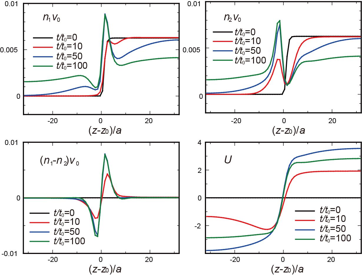
In Fig.3, we show the time development of $n_{1}$, $n_{2}$, $n_{1}-n_{2}$ in the very early stage, and $\Phi$, which illustrate establishment of the electric double layer in the time region $t<100t_{0}$. In this stage, the profiles of $\phi$ and $n_{i}$ are nearly one-dimensional and the surface undulations are negligible. We can see establishment of a large electric double layer, where the electric field is of order $k_{B}T/e$. The integral in eq.(23) is time-dependent here and may be regarded as an effective surface tension. It is about $0.2k_{B}T/a^{2}$ at $t=0$ and tends to a negative value of order $-0.05k_{B}T/a^{2}$ for $t>\kern-12.0pt\lower 5.0pt\hbox{$\displaystyle{\sim}$}50t_{0}$ in this case. Here, $\Delta U\sim 5$ and eq.(42) gives $k_{c}\sim 0.3a^{-1}$.

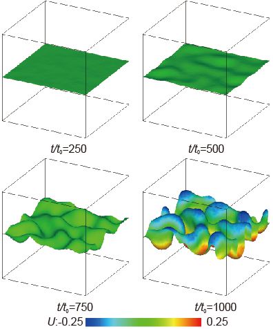
In Fig.4, we display slower time-evolution of interface deformations after the establishment of the electric double layer induced by antagonistic ion pairs at $t/t_{0}=250,500,750$, and 1000, where the domain size is of order $2\pi/k_{c}$ in accord with eq.(42). While the linear growth theory holds for $t<\kern-12.0pt\lower 5.0pt\hbox{$\displaystyle{\sim}$}500t_{0}$, the system is in the nonlinear growth regime with large surface disturbances at $t=1000t_{0}$. Note that this final time is of the order of the diffusion time $t_{D}=L^{2}/4D_{0}\sim 10^{3}t_{0}$. For $t\gg t_{D}$ the system should tend to a bicontinuous mesophase displayed in our previous paper [3].

5 Summary

We stress the crucial role of the selective solvation of a solute in phase transitions of various soft materials, which should be relevant in understanding a wide range of mysterious phenomena in water. Particularly remarkable in polar binary mixtures are mesophase formation induced by an antagonistic salt[4, 2, 3] and precipitation induced by a one-sided solute (a salt composed of hydrophilic cations and anions and a neutral hydrophobic solute)[11, 12]. Regarding the problem of mesophase formation, our theory is still insufficient and cannot well explain the complicated phase behavior disclosed by the experiments [13, 14, 15].

We propose experiments of the surface instability. For example, it should be induced around a droplet of pure water (oil) inserted in a bulk oil-rich (water-rich) region in the immisible condition, where the droplet or the surrounding region contains a small amount of an antagonistic salt. The previous experiments of droplet formation[25, 26] were performed in the strong segregation condition far from the solvent criticality and, as a result, the surface tension might have not been negative even after the formation of an electric double layer. Thus, experiments should also be performed on near-critical aqueous mixtures in two-phase coexistence, where a small amount of an antagonistic salt is added to either of the water-rich or oil-rich region as in Sec.4 of this paper.

This work was supported by KAKENHI (Grant-in-Aid for Scientific Research) from the Ministry of Education, Culture, Sports, Science and Technology of Japan. Thanks are due to informative discussions with R. Okamoto, K. Sadakane, and H. Seto.

References

• [1] J. N. Israelachvili, Intermolecular and Surface Forces (Academic Press, London, 1991).
• [2] T. Araki and A. Onuki, J. Phys.: Condens. Matter 21 (2009) 424116.
• [3] A. Onuki, T. Araki, and R. Okamoto, J. Phys.: Condens. Matter 23 (2011) 284113.
• [4] A. Onuki, R. Okamoto, and T. Araki, Bull. Chem. Soc. Jpn. 84 (2011) 569.
• [5] A. Onuki and H. Kitamura, J. Chem. Phys. 121 (2004) 3143.
• [6] A. Onuki, Phys. Rev. E 73 (2006) 021506.
• [7] I. Borukhov, D. Andelman, R. Borrega, M. Cloitre, L. Leibler, and H. Orland, J. Phys. Chem. B 104 (2000) 11027.
• [8] A. Onuki and R. Okamoto, J. Phys. Chem. B, 113 (2009) 3988.
• [9] R. Okamoto and A. Onuki, J. Chem. Phys. 131 (2009) 094905.
• [10] R. Okamoto and A. Onuki, Phys. Rev. E 84 (2011) 051401.
• [11] R. Okamoto and A. Onuki, Phys. Rev. E 82, 051501 (2010).
• [12] A. Onuki and R. Okamoto, Current Opinion in Colloid $\&$ Interface Science, 16 (2011) 525.
• [13] K. Sadakane, H. Seto, H. Endo, and M. Shibayama, J. Phys. Soc. Jpn., 76 (2007) 113602.
• [14] K. Sadakane,, A. Onuki, K. Nishida, S. Koizumi, and H. Seto, Phys. Rev. Lett. 103 (2009) 167803.
• [15] K. Sadakane, N. Iguchi, M. Nagao, H. Endo, Y. B. Melnichenko, and Hideki Seto, Soft Matter, 7 (2011) 1334.
• [16] G. Jones and W. A. Ray, J. Am. Chem. Soc. 59 (1937) 187; ibid. 63 (1941) 288; ibid. 63 (1941) 3262.
• [17] Y. Levin and J. E. Flores-Mena, Europhys. Lett. 56 (2001) 187.
• [18] A. P. dos Santos and Y. Levin, J. Chem. Phys. 133 (2010) 154107.
• [19] J. D. Reid, O. R. Melroy, and R.P. Buck, J. Electroanal. Chem. 147 (1983) 71.
• [20] G. Luo, S. Malkova, J. Yoon, D. G. Schultz, B. Lin, M. Meron, I. Benjamin, P. Vanysek, and M. L. Schlossman, Science, 311 (2006) 216.
• [21] J.W. Gibbs, Collected works, vol.1,pp.219-331 (1957), New Haven, CT: Yale University Press.
• [22] S.A. Safran, Statistical Thermodynamics of Surfaces, Interfaces, and Membranes (Westview Press, 2003).
• [23] A. Onuki, J. Chem. Phys. 128 (2008) 224704.
• [24] A. Onuki, Europhys. Lett. 82 (2008) 58002.
• [25] K. Aoki, M. Li, J. Chen, and T. Nishiumi Electrochem. Commun. 11 (2009) 239.
• [26] K. Wojciechowski and M. Kucharek, J. Phys. Chem. B, 113 (2009) 13457.
• [27] Le Quoc Hung, J. Electroanal. Chem. 115 (1980) 159.
• [28] J. Koryta, Electrochim. Acta 29, 445 (1984).
• [29] A. Sabela, V. Marecek, Z. Samec, and R. Fuocot, Electrochim.Acta, 37, 231 (1992).
• [30] T. Osakai and K. Ebina, J. Phys. Chem. B 102 (1998) 5691.
• [31] A. Hamnett, C. H. Hamann, and W. Vielstich, Electrochemistry (Wiley-VCH, Weinheim, 1998).
• [32] A. Onuki, Phase Transition Dynamics (Cambridge University Press, Cambridge, 2002).
• [33] P. Debye and K. Kleboth, J. Chem. Phys. 42 (1965) 3155.
• [34] E. H. Lucassen-Reynders and J. Lucassen, Adv. Colloid Interface. Sci. 2 (1969) 347.