A $Y$-BAND LOOK OF THE SKY WITH 1-M CLASS TELESCOPES

Abstract

$Y$-band is a broad passband that is centered at $\sim$1 $\mu m$. It is becoming a new, popular window for extragalactic study especially for observations of red objects thanks to recent CCD technology developments. In order to better understand the general characteristics of objects in $Y$-band, and to investigate the promise of $Y$-band observations with small telescopes, we carried out imaging observations of several extragalactic fields, brown dwarfs, and high redshift quasars with $Y$-band filter at the Mt. Lemmon Optical Astronomy Observatory and the Maidanak observatory. From our observations, we constrain the bright end of the galaxy and the stellar number counts in $Y$-band. We also test the usefulness of high redshift quasar ($z>$6) selection via $i-z-Y$ color-color diagram, to demonstrate that the $i-z-Y$ color-color diagram is effective for the selection of high redshift quasars even with a conventional optical CCD camera installed at a 1-m class telescope.

1 INTRODUCTION

Recently, there has been an enormous progress in the studies of Near-InfraRed (NIR) bright sources. Large area surveys such as the Sloan Digital Sky Survey (SDSS; Abazajian et al. 2009), the Two Micron All Sky Survey (2MASS; Skrutskie et al. 2006), the 2 degree Fields Galaxy Redshift Survey (2dFGRS; Colless et al. 2001), the UKIRT Infrared Deep Sky Survey (UKIDSS; Lawrence et al. 2007) and deep imaging observations from space and the ground led to the discovery of rare, interesting objects such as quasars at the epoch near re-ionization of the universe (Fan et al. 2000), the understanding of distant massive galaxies and clusters in formation (Kang & Im 2009; Shim et al. 2007), and the discovery of many brown dwarfs such as T/L-dwarfs with surface temperature around 1000 K or below (Chiu et al. 2007). Many of these studies start with extensive ground-based or space-based imaging observations in optical (from $u$-band to $z$-band, or 0.3551 $\mu m$ $-$ 0.8931 $\mu m$), or in NIR ($J$-band to $K$-band, or 1.27 $\mu m$ $-$ 2.2 $\mu m$) over a large-area in the sky, or very deeply in small fields. Spectroscopic observations have been carried out to unveil the true nature of interesting astronomical sources selected from the multi-wavelength imaging data. These previous studies have provided valuable multi-wavelength data-sets, but there still remains a gap in wavelength coverage between the optical and the NIR, namely 1 $\mu m$ wavelength region, which is much less explored compared to the other wavelengths.

The wavelength region of $Y$-band is centered at $\sim$1 $\mu m$ with a spread of about 0.1 $\mu m$ (Hillenbrand et al. 2002). The $Y$-band is located at a relatively clean atmospheric window between NIR and optical bands. Fig. 1 shows a typical $Y$-band filter transmission curve compared to other red, optical bands and $J$-band. The name $Y$ is dubbed to distinguish it from $z$ and $Z$ filters which cover the wavelength close to $Y$. Traditionally, this wavelength has been neglected mainly due to the lack of detectors that can cover this wavelength in a cost-effective way. But the situation is changing with the emergence of deep depletion CCD chips that boast excellent sensitivity at 1.0 $\mu$m (QE $\sim$ 25 $-$ 50%; e.g., Park et al. 2011), compared to those of the traditional back-illuminated, thinned CCDs (QE $\sim$ 5 $-$ 10%; e.g., Lee et al. 2010; Im et al. 2010). These CCDs are cost-effective compared to expensive NIR detectors made of InSb or HgCdTe, making observations with $Y$-band more popular than ever.

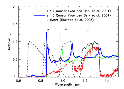
Fig. 1.—: Spectral Energy Distributions (SEDs) of a $z\sim$6 quasar (the solid blue line), $z\sim$7 quasar (the dotted green line) and L dwarf star (the red dot-dashed line). The black dashed lines represent the relative transmission efficiencies of $i,z,Y$, and $J$ filters. These types of objects have very red $i-z$ or $z-Y$ colors, and the addition of $Y$ or $J$-band helps to distinguish high redshift quasars from brown dwarfs.

Early works with $Y$-band were mainly limited to studies of cool and low mass stars like brown dwarfs. A pioneering work of Hillenbrand et al. (2002) attempted to provide photometric calibration for $Y$-band, and demonstrated the usefulness of $Y$-band for studying cool stars. $Y$-band is useful for the identification of low-mass stars especially at young ages, and can distinguish low mass stars from high mass stars even in the galactic plane and in star-forming regions without too much interruption due reddening.

Also, extragalactic research can benefit from $Y$-band imaging greatly. These days, the forefront of the extragalactic astronomy is moving toward the high redshift universe at $z>$ 6. Discoveries of high redshift quasars and galaxies provide prospects to understand the star formation and the re-ionization history of universe. The assembly history of massive galaxies at 1 $<z<$ 3 is another important topic of extragalactic study. It appears that massive, red galaxies are already in place at $z\sim$ 1 (Im et al. 2002), and a significant build-up of massive galaxies at $z>$ 1 is hinted from the deep extragalactic surveys (Drory et al. 2005; Shim et al. 2007). In order to improve our understanding on the above issues, we need more work in NIR.

Through $Y$-band observation, we can study various extragalactic objects like high redshift quasars and galaxies ($z>$ 6), and improve photometric redshift determination of red galaxies at $z>1$ that have their 4000$\AA$ breaks redshifted to $Y$-band. Finding quasars and galaxies at $z>6$ is important since they can provide ways to investigate the cosmic re-ionization epoch. Going further than $z>6.5$ is even more important, as they allow us to probe the universe at an earlier epoch but the number of known quasars at $z>6.5$ is only handful so far (Mortlock et al. 2011). Fig. 1 demonstrates how NIR band observation is crucial especially in $Y$-band for high redshift quasar search. High redshift quasars and galaxies have a strong spectral break at Ly$\alpha$. The Ly$\alpha$ is redshifted to $z$ or $Y$-bands when the objects are at $z>6$ or at $z>7$, allowing us to use this feature to identify high redshift objects. $Y$-band enables us not only to identify the spectral break but also to measure the spectral shape long-ward of the Lyman break to distinguish high redshift objects from brown dwarfs. Similarly, adding an NIR point to Gamma-Ray Burst (GRB) follow-up observation in optical band is one of useful aspects of $Y$-band. Just like high redshift quasar search, it helps in determining redshifts of GRBs, especially those at $z>$ 6.5, by the Lyman break dropout technique (Steidel et al. 2003). Hence, recent large surveys like UKIDSS (Lawrence et al. 2007) and Pan-STARRS surveys adopt $Y$-band.

Considering the emergence of $Y$-band, we performed $Y$-band imaging observations of well-known extragalactic fields using the 1-m telescope at Mt. Lemmon Optical Astronomy Observatory (LOAO) in Arizona, USA, and the 1.5-m telescope at the Maidanak observatory in Uzbekistan. Our scientific goals are primarily three folds. The first goal is to establish the number count of $Y$-band objects at a relatively bright magnitude limit, but faint enough to go beyond the surveys such as UKIDSS Large Area Survey (LAS). So far no work has been carried out to understand the number count study in $Y$-band. This study will be the first work which will establish the $Y$-band number count at bright end. Our number counts can be used to check the completeness of the other shallower surveys, and can offer a first look of the nature of sources in $Y$-band, especially at bright-end part. We will also check the limiting magnitudes at a given exposure time for the small telescopes we used, and gauge the usefulness of such observations for the study of distant extragalactic sources. The second goal is to test the selection of high redshift quasars using $i-z$ vs $z-Y$ plot. We obtained the $Y$-band imaging observation of the known high redshift quasars and cool dwarfs. For this study, we target $z>$ 5.8 SDSS quasars and cool dwarfs. Previous studies used $J$-band for this purpose, but we will show that $Y$-band can substitute the $J$-band point, therefore, making it possible to carry out an efficient selection of high redshift quasar candidates even with small telescopes equipped with traditional CCD cameras. The third goal is to provide photometric calibration parameters in $Y$-band. We will provide the basic photometric calibration in $Y$-band at the two optical observatories.

We will first describe the facilities we used for our observation, followed by the observation, the reduction, and the analysis of the data. Then, the photometric calibration, and the source counts will be introduced. We will construct the color-color diagram for high redshift quasars and cool brown dwarfs, in order to directly test the usefulness of the selection method for the high redshift quasars. Discussion on the implications of our findings will be followed by the summary of this work.

2 $Y$-BAND FILTER AND OBSERVATION

We carried out the $Y$-band imaging observations using the LOAO 1-m telescope and its 2k CCD camera, as well as the Maidanak 1.5-m telescope and its 4k CCD camera, SNUCAM (Im et al. 2010). These observations and the instrument characteristics are described below.

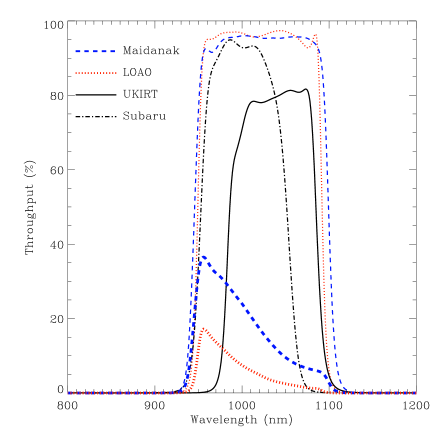
Fig. 2.—: The $Y$-band filter transmission curves and the throughputs of LOAO and Maidanak observatory. The thin lines represent the filter transmission curve only. The thick lines show the throughput including the detector QE (the blue-dashed line for SNUCAM, and the red-dotted line for the LOAO CCD camera). Note that the transmission curve of our $Y$-band filters is slightly different from those of the UKIRT WFCAM $Y$-band and z_R filter of Subaru Suprime-Cam.

Table 1. : Target fields and summary of observation

Target	R.A.	Dec.	Exp. time	Area	Detection limit
field	(J2000)	(J2000)	($\times$ 300s)	deg2	5$\sigma$ (AB mag)
NEPc	02:18:00	-07:00:00	18.8-21.6	0.1	21.2
CFHTLS-W1c	17:56:27	66:12:45	26.8-28	0.1	21.1
GRB 090429Bc	14:02:40	32:10:14	36	0.1	22.3
EGS	14:19:00	52:47:30	50	0.12	20.76
FLS	17:21:00	60:17:00	18	0.12	20.52
NEP	17:55:30	66:25:00	3-52	0.96	19.49-20.94
UKIDSS	12:00:00	00:00:30	8	0.12	19.91
SDSS J113717+354956.9a	11:37:22	35:49:57	8	0.12	19.0
SDSS J084035+562419.9a	08:40:35	56:24:20	18	0.12	20.5
SDSS J084119+290504.4a	08:41:20	29:05:00	15	0.12	20.3
SDSS J092721+200123.7a	09:27:21	20:01:23	16	0.12	20.3
SDSS J125051+313021.9a	12:50:51	31:30:22	17	0.12	20.5
SDSS J065405+652805.4b	06:54:05	65:28:05	14	0.12	20.3
SDSS J083506+195304.3b	08:35:06	19:53:04	10	0.12	19.5
SDSS J104335+121314.1b	10:43:35	12:13:14	10	0.12	19.4
SDSS J121951+312849.4b	12:19:51	31:28:49	10	0.12	19.7
SDSS J090900+652527.1b	09:09:00	65:25:27	8	0.12	18.5

^a: SDSS quasar

^b: SDSS brown dwarf

^c: Observed at Maidanak

2.1 $Y$-band Filters

The $Y$-band filters were manufactured by Asahi Spectra Inc. with a custom specification. The $Y$-band filter for the LOAO 1-m has a physical size of roughly 3 $\times$ 3 inches (square shaped), and the Maidanak filter has a physical size of 4 $\times$ 4 inches to accommodate the large 4k $\times$ 4k array. Both filters are about 1 cm thick. Two glasses are cemented each other to create the necessary transmission curve. The LOAO $Y$-band filter was installed on the telescope at February 2008, while the Maidanak $Y$-band filter was installed in the summer of 2008. After the installation of the $Y$-band filter at the Maidanak observatory, we also carried out test observations which will be described below. The filter transmission curves of our $Y$-band filters are plotted in Fig. 2 which is almost identical to the Pan-STARRS $Y$-band filter. For comparison, $Y$-filters of UKIRT are plotted over the former.

2.2 LOAO Observation

2.2.1 Targets

The main purposes of the LOAO observation were to understand the characteristics of the $Y$-band sky especially for the study of distant, extragalactic objects and checking the usefulness of $Y$-band observations for high-redshift quasar selection. Therefore, we chose target fields with the existing multi-band data. The fields chosen are the Extended Groth Strip (EGS; Davis et al. 2007), the First Look Survey field (FLS; Fadda et al. 2006), the AKARI North Ecliptic Pole (NEP) survey field (Matsuhara et al. 2006; Lee et al. 2007), and a part of a UKIDSS LAS field. The EGS is a field near the constellation Ursa Major, which boasts of a wealth of the multi-wavelength datasets from X-ray to radio including HST, Chandra, AKARI (Song & Im 2009), and a large number of spectroscopic redshifts taken by DEEP and DEEP2 surveys (Vogt et al. 2005; Im et al. 2002; Faber et al. 2007). The Spitzer FLS is the first extragalactic survey carried out by the Spitzer Space Telescope at the wavelengths of 3.6, 4.5, 5.6, 8.0, 24, 70, and 160 $\mu m$, with the ancillary data from UV to Radio, including the Canada France Hawaii Telescopes (CFHT) MegaCam images in $u$-band and $g$-band taken by our group (Shim et al. 2006). The UKIDSS field is chosen for comparison to our $Y$-band observation. The AKARI NEP survey field is centered on the ecliptic pole, and it also boasts a wide range of multi-wavelength datasets centered on the AKARI IR data.

Additionally, 5 SDSS quasars at $z>$ 5.8 and 5 brown dwarfs (T and L dwarfs) were observed to verify the selection method to distinguish between high redshift quasars and brown dwarfs on a color-color diagram. For a few cases, $z$-band data were taken to examine the performance of the $z$-band imaging of the LOAO 1-m telescope. For standard star, we chose A0V stars from HIPPARCOS (Perryman et al. 1997) catalog because there are very few standard stars in $Y$-band. The A0V stars allow us to immediately calibrate the photometric zero-point, since A0V stars have 0 colors in the Vega magnitude system. The observed fields are summarized on the Table 1. The total observed area of LOAO fields spans about 2 deg².

2.2.2 Observation

We used the LOAO 2k CCD camera system for the observations, which was manufactured by Finger Lakes Instrumentation with a KAF-4301E chip made by KODAK, Inc.. Its 24 $\mu m$ $\times$ 24 $\mu m$ scale translates to a pixel size of 0.64^′′, providing a field of view of 22^′ $\times$ 22^′ on the 1-m telescope. The telescope and the camera are remotely controlled from Korean Astronomy & Space Institute (KASI), Korea. The front-illuminated CCD of LOAO does not suffer from fringing at 1 $\mu m$ compared to back-illuminated thinned CCD chips.

Observations were carried out on the nights of 2008 March 19-23 and July 16-19, for a total of 9 nights. Average seeing was 2.5^′′, although some of the frames were taken with slightly out of focus. The data was taken with exposures exceeding 2 min. The moon phase was full but this did not affect the sensitivity too much just like any other NIR observation. In the period of 9 nights, the weather was clear on 5 nights, cloudy on 4 other.

When guide stars were not found easily, the observation was done without guiding and the exposure per frame was limited to 2 minutes or less. The observation was done by dithering with each dither pattern having 20^′′ - 30^′′ steps. This procedure was necessary due to many hot or warm pixels and bad columns in the 2k CCD camera whose intensities varied with time. The total integration time was set to 1 hr per field (plus the overhead of about 30 min). In some fields, we divided the region into several tiles to cover a wide area.

The standard stars were observed every night except on 16 July at various airmasses as the weather permitted. The standard star observation summary is given in Table 2. We also obtained the bias frames, dark frames for calibration, as well as the sky flats. Due to the low efficiency of the CCD camera at $Y$-band, we note that a relatively long exposure was needed for obtaining $Y$-band flat, which were taken usually between $R$-band and $V$-band flats.

2.3 Maidanak Observation

2.3.1 Targets

The observed target fields are the AKARI NEP survey field, a small part of the XMM-LSS field of the CFHT Legacy Survey (Cuillandre & Bertin 2006) for which $ugriz$ imaging data are available. The CFHTLS field overlaps with the UKIDSS Deep eXtragalactic Survey (DXS; Lawrence et al. 2007) area. Finally, GRB 090429B was observed in $Y$-band as a part of GRB follow-up observation campaign (e.g., Lee et al. 2010) with a 3 hr total integration which corresponds to the deepest $Y$-band imaging data obtained by this work. Some of the AKARI NEP fields were covered at Maidanak as well. The observed fields are summarized in Table 1.

2.3.2 Observation

The observation was carried out using SNUCAM on the 1.5-m telescope (Im et al. 2010) during August 30, 2008 through September 4 for 6 nights, except for the GRB 090429B field. SNUCAM is a cryo-cooled CCD camera with a back-illuminated, thinned 4k $\times$ 4k CCD chip manufactured by Fairchild, Inc. On the 1.5-m telescope, SNUCAM has a pixel size of 0.266^′′, and the field of view of 18^′ $\times$ 18^′. The weather conditions during the observation were generally good, but we accumulated the data worth about two nights due to operation problems with the telescope. The average seeing was 1.2^′′, although some of the frames were taken slightly out of focus. The exposure per frame was limited to 2 minutes or less because of tracking instability and the need for dithering. The observation was done by dithering with each dither pattern having 20^′′ - 30^′′ steps. This procedure was necessary due to fringing which is typical for a back-illuminated, thinned CCD chip. We observed A0V stars from the HIPPARCOS catalog as standard stars for most cases and a UKIRT faint standard star (P272-D) when we observed GRB 090429B. We also obtained the bias frames, and flat frames for calibration.

Table 2. : Observed standard star list

Date	Standard	R.A.	Dec.	Exp. time	Airmass	Zero	$V$ mag	E($B-V$)	AV
(2008)	star	(J2000)	(J2000)	[second]	sec(Z)	point	Vega)	[mag]	[mag]
Mar. 20	HIP 32549	06:47:28	44:19:53	20	1.256	18.10	8.24	0.066	0.219
	HIP 71172	14:33:23	69:37:44	60	1.075	18.41	6.06	0.016	0.053
Mar. 21	HIP 32549	06:47:28	44:19:53	20	1.258	18.25	8.24	0.066	0.219
	HIP 33297	06:55:34	08:19:27	10	1.096	18.14	9.74	0.220	0.731
	HIP 42853	08:43:56	19:02:03	20	1.071	18.53	8.30	0.029	0.095
	HIP 71172	14:33:23	69:37:44	20	1.193	18.34	6.06	0.016	0.053
Mar. 22	HIP 32549	06:47:28	44:19:53	20	1.270	18.20	8.24	0.066	0.219
	HIP 34107	07:24:20	01:29:18	10	1.182	18.28	6.57	0.364	1.206
	HIP 42853	08:43:56	19:02:03	20	1.040	18.62	8.30	0.029	0.095
	HIP 42853	08:43:56	19:02:03	20	1.777	18.57	8.30	0.029	0.095
	HIP 71172	14:33:23	69:37:44	20	1.221	18.40	6.06	0.016	0.053
Mar. 23	HIP 32549	06:47:28	44:19:53	20	1.261	18.21	8.24	0.066	0.219
	HIP 34107	07:24:20	01:29:18	12	1.168	18.23	6.57	0.364	1.206
	HIP 42853	08:43:56	19:02:03	20	1.062	18.55	8.30	0.029	0.095
	HIP 42853	08:43:56	19:02:03	25	1.378	18.54	8.30	0.029	0.095
Mar. 24	HIP 32549	06:47:28	44:19:53	20	1.272	18.23	8.24	0.066	0.219
	HIP 34107	07:24:20	01:29:18	12	1.182	18.24	6.57	0.364	1.206
	HIP 42853	08:43:56	19:02:03	30	1.042	18.53	8.30	0.029	0.095
	HIP 42853	08:43:56	19:02:03	30	1.596	18.48	8.30	0.029	0.095
Jun. 18	HIP 88429	18:03:14	19:36:47	10	1.360	18.00	6.41	0.099	0.327
Jun. 19	HIP 65599	13:26:58	11:54:30	20	1.081	18.01	7.99	0.027	0.091
	HIP 75230	15:22:23	12:34:03	12	1.107	18.04	6.41	0.043	0.144
	HIP 88429	18:03:14	19:36:47	10	1.176	18.12	6.41	0.099	0.327
	HIP 88429	18:03:14	19:36:47	10	1.557	18.07	6.41	0.099	0.327
Jun. 20	HIP 65599	13:26:58	11:54:30	20	1.077	18.08	7.99	0.027	0.091
	HIP 88429	18:03:14	19:36:47	10	1.373	18.06	6.41	0.099	0.327
	HIP 88429	18:03:14	19:36:47	10	1.636	18.11	6.41	0.099	0.327
Aug. 30	HIP 98460a	20:02:05	12:19:19	10	1.378	19.10	9.38	0.203	0.674
	HIP 98460a	20:02:05	12:19:19	20	1.208	19.17	9.38	0.203	0.674
	HIP 111538a	22:35:48	40:05:27	20	1.149	18.94	9.48	0.127	0.570
	HIP 111538a	22:35:48	40:05:27	20	1.056	18.94	9.48	0.127	0.570
	HIP 582a	00:07:05	60:23:33	20	1.266	19.24	9.52	0.959	3.178
Aug. 31	HIP 98460a	20:02:05	12:19:19	20	1.462	19.10	9.38	0.203	0.674
	HIP 98460a	20:02:05	12:19:19	20	1.197	19.10	9.38	0.203	0.674
	HIP 111538a	22:35:48	40:05:27	20	1.207	18.94	9.48	0.127	0.570
	HIP 111538a	22:35:48	40:05:27	20	1.051	18.93	9.48	0.127	0.570
	HIP 582a	00:07:05	60:23:33	20	1.271	19.26	9.52	0.959	3.178
Apr. 29	P272-Da	14:58:33.1	37:08:33	30	1.050	20.12	11.839	0.020	0.067
(2009)	(MKO)						($Y$ mag)

^a: Observed at Maidanak

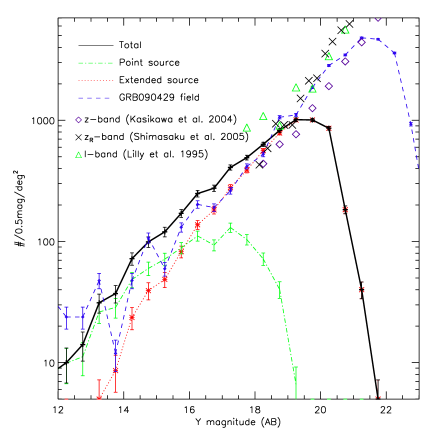
Fig. 3.—: The number counts of $Y$-band sources. For comparison, the observed number counts from literatures are shown for $I$-band (green triangles), $z$-band (black crosses) and $z_{R}$-band (purple diamonds). The shallow $Y$-band counts ($Y<18.5$ mag) are constructed from all the fields we observed (total area of $\sim$2 deg²). The number count in the GRB 090429B field, which is the deepest among the observed fields, is shown with the blue dashed line (0.08 deg²).

3 DATA REDUCTION

3.1 Image Reduction and Stacking

We used IRAF packages for pre-processing and stacking of the data. We describe the data reduction procedure below.

3.1.1 LOAO data

Fig. 4.—: Completeness test of an EGS field

The reduction follows a standard procedure of the bias and the dark subtraction, followed by the flat-fielding. To create a master bias image for each night, 40 bias frames were combined. Master darks are constructed from the darks taken with the same exposure times as the science frames. The dark subtraction was crucial to remove many of the bad pixels and bad columns. Flat fields were constructed using skyflats taken during twilight. The peak-to-peak variation of the skyflat is measured to be 0.8 - 1.4.

The reduction process removes most of the artificial features on the image, but some of the time-variable bad pixels remain which are removed later by stacking of the dithered frames. A large scale pattern remains at 3% level, peak-to-peak. We suspect that this large scale pattern arises mostly from imperfect flat-fielding where the flat-field data rely on the data taken in a couple of nights. Overall, we believe that our photometry has an intrinsic uncertainty of about 3% level (0.03mag) due to the flat-field variation.

For registration of the reduced, dithered images, we selected non-saturated stellar objects with good Gaussian profiles as registration stars, and performed the registration and image shift using imalign procedure. The registered images were stacked in median after subtracting the background level determined to be a mode of the pixel value distribution of each image. Cosmic ray rejection (crrejct) was applied during the stacking process.

3.1.2 Maidanak data

The procedure of the Maidanak SNUCAM data reduction follows that of Jeon et al. (2010). This is similar to the LOAO data reduction procedure, but with a few differences.

The SNUCAM data do not require dark subtraction since SNUCAM has virtually no dark current at the operating temperature. On the other hand, it requires additional subtraction of the background level in the four quadrant readout channels. Also, the fringing pattern needs to be removed which is severe in $Y$-band images.

Flat fields were constructed using skyflats taken during twilight. The number of skyflats was typically 3 - 5, and these were combined by setting the flatcombine parameter of zero to “mode”. The peak-to-peak variation of the skyflat is measured to be 0.98 - 1.02. The reduction process removes most of the artificial features on the image, although a large scale pattern remains at more than 5% level due to fringing. To correct the fringe patterns, we created a master fringe frame by stacking all of the bias-subtracted, flat-fielded object frames in median without performing registration. The master fringe frame was scaled by the sky-background level of each science frame and subtracted from the object frame (see also Jeon et al. 2010). After the fringe correction, the images were registered and stacked in the same way as the LOAO images.

3.2 Photometry Calibration

We measured the flux of the standard stars to get photometric parameters in $Y$-band. A standard equation as below is used for deriving the photometry calibration parameters, $\xi$ (zero-point), $\kappa$ (atmospheric extinction coefficient).

$$\xi=m_{0}+2.5\,log(DN/sec)+\kappa(X-1)$$ (1)

Here $m_{0}$ is a known V magnitude of an A0V star, and $X$ is the airmass which is equal to sec(z) where z is the zenith distance. By definition, A0V star’s color is zero. The color-term is ignored here. Aperture photometry of a standard star observed twice in a day was used to calculate $\kappa$ and $\xi$ at different airmass values. The total flux of a star is obtained with an aperture diameter of 14^′′, to minimize the flux loss. The sky was estimated using an annulus of 28^′′ diameter, with a width of 7^′′. The photometry calibration results are summarized in Table 2. We note that the atmospheric extinction coefficient, $\kappa$, has a value between 0.05 and 0.1, and we take the average of these values as a measure of $\kappa$ for the nights where no standard star data were taken. In this way, we find that the atmospheric extinction coefficients are $\kappa$ = 0.087 for LOAO, $\kappa$ = 0.1 for Maidanak observatory. The zero point, $\xi$, is calculated for each standard star. We find that the zero points vary between different standard stars by as much as 0.5 mag in some cases. We attributed this to be due to the weather conditions, the uncertainty in E(B-V) corrections, as well as the variability of standard stars in some cases. For example, the data were taken with thin clouds present for the March 18-20 data, which resulted in a relatively bright zero point value. We also found that some of the standard star data were a little out-of-focus, and the photometry of such stars seem spurious. Overall, the zero-points were allowed to vary between day-to-day, and it ranges between $\xi$ = 18.1 - 18.5 in LOAO, $\xi$ = 18.9 - 19.3 in Maidanak. We expect the uncertainty in the zero-point to be within 0.1 magnitude through comparison of zero-points from various standard stars within a single night.

3.3 Astrometry Calibration

Astrometry was done with SCAMP and SWarp software (Terapix; Bertin 2008) with stars in the United State Naval Observatory (USNO-B1; Monet et al. 2003) catalog as reference stars. After astrometry calibration, the rms error of astrometry is computed to be less than 0.35^′′ from the SCAMP software. After the astrometry calibration we updated the header of image files using SWarp.

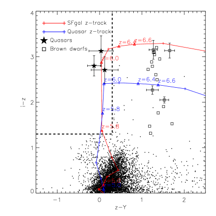
Fig. 5.—: Color-color plot in $i-Y$ vs $z-Y$. Black stars are known quasar at $z$ $\sim$ 6. Open squares with error bars are brown dwarfs and other open squares without error bars are L/T dwarf stars taken from Hewett et al. (2006). Black dots are other sources from the observed data such as stars and galaxies. Blue solid line is an evolutionary track of star forming galaxy and red line is that of a quasar.

3.4 Source Detection and Extraction

SExtractor (Bertin & Arnouts 1996) was used for the object detection and photometry. The magnitude zero-points of standard stars are adopted as in Table 2 for each night. The DETECTION THRESHOLD is set to 1.2$\sigma$ and the MINIMUM AREA to be 4 pixels. The background mesh size of 32 $\times$ 32 pixels is adopted for estimating local background. The parameters were chosen so that we minimize the spurious detections as well as making sure any obvious objects were not missed through the eye-ball inspection of the image. In general, about 2000 objects are detected per field with $\sim$ 1 hr total integration. We adopt the Auto magnitude from SExtractor. To transform the Vega magnitude system to AB magnitude system, we adopted the relation of $Y_{AB}$ mag= $Y_{Vega}$ mag + 0.63 from Hewett et al. (2006).

4 RESULTS

Table 3. : Number counts

$Y$ magnitude	Total a	Extended source a	Point source a	GRB 090429B a
(AB mag)	(deg-2)	(deg-2)	(deg-2)	field (deg-2)
11.5$-$12.0	8.0 $\pm$ 2.8	0.0 $\pm$ 0.0	8.0 $\pm$ 2.8	35.7 $\pm$ 5.9
12.0$-$12.5	10.0 $\pm$ 3.2	0.1 $\pm$ 0.3	9.9 $\pm$ 3.2	23.8 $\pm$ 4.8
12.5$-$13.0	14.1 $\pm$ 3.8	2.9 $\pm$ 1.7	11.2 $\pm$ 3.4	23.8 $\pm$ 4.8
13.0$-$13.5	31.2 $\pm$ 5.6	5.0 $\pm$ 2.2	26.2 $\pm$ 5.1	47.6 $\pm$ 6.9
13.5$-$14.0	37.2 $\pm$ 6.1	8.6 $\pm$ 2.9	28.6 $\pm$ 5.3	11.9 $\pm$ 3.45
14.0$-$14.5	72.1 $\pm$ 8.5	23.6 $\pm$ 4.9	48.5 $\pm$ 7.0	47.6 $\pm$ 6.9
14.5$-$15.0	99.2 $\pm$ 10.0	39.3 $\pm$ 6.3	59.9 $\pm$ 7.7	107.1 $\pm$ 10.35
15.0$-$15.5	120.1 $\pm$ 11.0	48.6 $\pm$ 7.0	71.5 $\pm$ 8.5	59.5 $\pm$ 7.7
15.5$-$16.0	170.7 $\pm$ 13.1	82.4 $\pm$ 9.1	88.4 $\pm$ 9.4	130.9 $\pm$ 11.4
16.0$-$16.5	248.4 $\pm$ 15.8	137.3 $\pm$ 11.7	111.1 $\pm$ 10.5	202.4 $\pm$ 14.2
16.5$-$17.0	275.3 $\pm$ 16.6	182 $\pm$ 13.5	93.3 $\pm$ 9.7	190.5 $\pm$ 13.8
17.0$-$17.5	408.2 $\pm$ 20.2	277.8 $\pm$ 16.7	130.4 $\pm$ 11.4	261.9 $\pm$ 16.2
17.5$-$18.0	492.1 $\pm$ 22.2	388.2 $\pm$ 19.7	103.8 $\pm$ 10.2	416.7 $\pm$ 20.4
18.0$-$18.5	633.9 $\pm$ 25.2	562.1 $\pm$ 23.7	71.8 $\pm$ 8.5	523.8 $\pm$ 22.9
18.5$-$19.0	825.9 $\pm$ 28.7	785.7 $\pm$ 28.0	40.2 $\pm$ 6.3	1059.5 $\pm$ 32.5
19.0$-$19.5	1012.4 $\pm$ 31.8	1005.8 $\pm$ 31.7	6.6 $\pm$ 2.6	1107.1 $\pm$ 33.3
19.5$-$20.0	1006.6 $\pm$ 31.7	1006.6 $\pm$ 31.7		1869.1 $\pm$ 43.2
20.0$-$20.5	860.0 $\pm$ 29.3	860 $\pm$ 29.3		2833.3 $\pm$ 53.2
20.5$-$21.0	183.0 $\pm$ 13.5	183 $\pm$ 13.5		3464.3 $\pm$ 58.8
21.0$-$21.5	40.0 $\pm$ 6.3	40.0 $\pm$ 6.3		4797.6 $\pm$ 69.2
21.5$-$22.0	5.0 $\pm$ 2.2	5.0 $\pm$ 2.2		4666.7 $\pm$ 68.3
22.0$-$22.5				3595.2 $\pm$ 59.9
22.5$-$23.0				928.6 $\pm$ 30.4

^a The errors are calculated assuming Poisson noise.

4.1 Number Counts

We derived the $Y$-band number counts from various fields (Fig. 3 and Table 3). Note that the error bars represent the Poisson errors. When deriving the number counts, we used counts from each field down to 10$\sigma$ detection limit. The number counts are also divided into the point and the extended sources. Point sources are classified by STELLARITY value larger than 0.8 given from SExtractor (down to $Y\sim 19$ mag), the remainder which have value less than 0.8 are classified as extended sources. We plot the number counts of the point sources with a green dot-dashed line and the extended sources with a red dotted line. The number counts of the GRB 090429B field was plotted independently (blue dashed line), since this field is much deeper than the other fields. We summarize the number counts in Table 3. The figure shows that the number counts at the bright end is dominated by stars and at the faint end is dominate by extended sources (galaxies). The faint-end number counts somewhat mimic those of $I$-band number counts. The number of sources down to $Y$=20 mag is roughly 800 per deg².

4.2 Completeness Test

We test the completeness using an EGS field. We created artificial stars and galaxies at magnitude range of 12 - 22 and placed them on the observed image, using the IRAF tasks of starlist, gallist and mkobjects. 40% of the extended sources are chosen as elliptical galaxies and the others as disk galaxies. Then, we checked to see how many of them could be detected with the same configuration of source detection as what we adopted for the source detection parameters as described in Section 3.4. Fig. 4 shows that this field has 50% completeness at 20.5 mag which is consistent with 5$\sigma$ depth of the EGS field in Table 1.

4.3 High Redshift Quasar Selection

One of the main motivations for this $Y$-band study is to test the effectiveness of the $Y$-band imaging for the selection of high redshift quasars. Here, we plot the $i-z$ versus $z-Y$ colors of sources in the extragalactic fields in Fig. 5. In the plot, we show high redshift quasars (z $\sim$ 5.8) with filled stars, and T/L dwarfs with squares. The expectation from Fig. 1 is that high redshift quasars have very red $i-z$ colors, while their $z-Y$ colors should be roughly flat (around 0). On the other hand, the steep SED slope of T/L dwarfs make them look very red in $i-z$ color like high redshift quasars, but they are also red in $z-Y$ colors. This point is clearly demonstrated in Fig. 5. Both high redshift quasars and T/L dwarfs are very red objects in $i-z$ colors, but in the plot we can separate them from each other since the cool dwarfs are redder than the high redshift quasars in $z-Y$ colors.

Previously, Fan et al. (2001, 2002) established a color-color space to select high redshift quasar candidates using the $i-z$ versus $z-J$ color-color diagram. Our result here demonstrates that a similarly effective exclusion of T/L dwarf stars from high redshift quasar candidates is possible, even with a $i-z$ versus $z-Y$ color-color diagram.

Our result justifies the use of a moderate sized telescope with a simple CCD camera, even for the selection of the highest redshift quasar candidates.

5 DISCUSSION

5.1 Detection Limits of LOAO and Maidanak Telescopes

Small telescopes are on disadvantage when studying faint sources at high redshift compared to large telescopes. However, for sources sufficiently bright such as quasars and GRBs, small telescopes can make an impact as long as the integration time to provide enough S/N is not too long. This is because, the observing times are much more readily available for small telescopes.

Fig. 6 shows the integration time versus 5$\sigma$ detection limits (in AB magnitude) for the LOAO and the Maidanak facilities. We see that the Maidanak telescope goes deeper, but not much deeper than the LOAO depth, despite the larger aperture of the mirror. The main culprit for the inefficiency of the Maidanak is the dusty primary mirror which is sometimes way over-due for the mirror coating and cleaning. The mirror of Maidanak 1.5m telescope was cleaned in 2009, after that we can see a marked improvement in depth through the observation of the GRB 090429B field.

The improvement is 1 mag deeper than before clearing in $Y$-band.

High redshift quasar candidates, such as SDSS $i$-band dropouts at 5.8 $<z<$ 6.5, typically have $z<$ 20.2 AB mag. Therefore, it is sufficient to detect objects brighter than $Y\sim$ 20 AB mag in order to enable efficient filtering of L/T-dwarfs. Actually, the magnitude limit can be brighter for the filtering of the L/T-dwarfs, since they are much brighter in the $Y$-band than z $\sim$ 6 quasars for a given $z$-band magnitude. The required $Y$-band magnitude limit can be achieved at about 1 hr exposure time on a clear night with the LOAO 1-m telescope even at a bad seeing, and much less than 1 hr with SNUCAM at the 1.5m assuming that it has a clean mirror. We expect that the observations at LOAO and Maidanak using $Y$-band filters can greatly help reduce our reliance on the $J$-band imaging for high redshift quasar candidate selection.

GRBs at high redshift can be detected with $Y$-band too. For example, GRB 050904 at $z=6.3$ (Haislip et al. 2006) was as bright as $Y\sim 18.7$ AB mag at 3 hrs post-burst, and $Y\sim 20.6$ AB mag at 0.5 days post-burst. Detection of such an event is possible at a few minutes (Maidanak) to a few tens of minutes (LOAO) shortly after the burst, and at 1$-$3 hrs exposure time even at $\sim 0.5$ days post-burst.

Fig. 6.—: 5$\sigma$ detection limits (AB mag) at a given exposure time. Open squares are for the LOAO limits, asterisks are for the Maidanak limits. A quasar at z $\sim$ 6 and GRB 050904 at z $\sim$ 6.3 are marked as horizontal dot-dashed lines. Diagonal dotted lines represent detection limits for Maidanak (the upper line) and for LOAO (the lower line). We indicate the $z$-band depth of 2 hr integration time at Maidanak for comparison which is located above 23 magnitude. The deepest $Y$-band Maidanak detection limit indicates the value derived from GRB 090429B.

5.2 Promises of $Y$-band Imaging with Small Telescopes

There are several interesting sciences that can be potentially carried out by a moderate sized telescope. First, a rapid response observation of GRB afterglow events, especially for those suspected to be occurring at high redshift, is interesting. The GRB afterglow has been identified out to z $\sim$ 9.4 (Cucchiara et al. 2011), and it is in principle possible to identify an afterglow at much higher redshifts. For GRB afterglows such as $i$-band or $z$-band dropouts, a combination of $i$-band / $z$-band / $Y$-band observation should be able to identify their redshift nature. Even at a moderate $\sim$10 minute exposure time, our observations suggest that we can detect GRB afterglows at 18-19 magnitude level using the LOAO 1.0-m or Maidanak 1.5-m telescopes.

$Y$-band observation can also provide an interesting data point in studying the SED of dusty GRBs. Recently, a high redshift GRB at $z\sim 5$ was identified to harbor supernova-produced dust (Perley et al. 2010; Jang et al. 2011). $Y$-band was one of key data points for distinguishing the extinction curve of supernova-produced dust from the dust extinction curves of other origins.

6 SUMMARY

We carried out $Y$-band imaging observations of extragalactic fields using 1-m class telescopes at LOAO and Maidanak observatory. The total observed area was $\sim$ 2 deg², and we reached $Y$ = 23 AB mag depth with 3 - 4 hour integration with the Maidanak 1.5-m telescope. We obtained photometric calibration data and derive the atmospheric extinction coefficient $\kappa$ = 0.087 at LOAO, and $\kappa$ = 0.1 at Maidanak observatory in $Y$-band from A0V standard stars. We present the number counts of $Y$-band sources which provide a useful constraint at the bright end of the number count. At a very bright end, point-like sources dominate the number count, while the faint end number count is dominated by galaxies. The color-color diagram $i-z$ vs. $z-Y$ is confirmed to be effective for discriminating high redshift quasars (z $>$ 6) from brown dwarfs. With the versatility and the availability of 1-m class telescopes, an 1-m class telescope can be useful for studying high redshift quasars and GRBs, and other red sources, once its capability is enhanced with a unique device such as $Y$-band filter.

ACKNOWLEDGMENTS We acknowledge the support from the National Research Foundation of Korea (NRF) grant funded by the Korean government (MEST), No. 2010-0000712. This work made use of the data taken with the LOAO 1-m telescope operated by KASI and the Maidanak 1.5-m telescope in Uzbekistan. We thank CEOU members for their help with useful advices, and the staffs of the Maidanak observatory and KASI for their assistance during our observation.

References

- Abazajian et al. (2009) Abazajian., et al. 2009, The Seventh Data Release of the Sloan Digital Sky Survey, ApJS, 182, 543
- Bertin & Arnouts (1996) Bertin, E., & Arnouts. 1996, SExtractor: Software for Source Extraction, A&AS, 117, 93
- Bertin (2008) Bertin, E. 2008, SWarp v2.17.0 Users guide
- Burrows et al. (2003) Burrows, A., et al. 2003, Beyond the T Dwarfs: Theoretical Spectra, Colors, and Detectability of the Coolest Brown Dwarfs, ApJ, 596, 587
- Chiu et al. (2007) Chiu, K., et al. 2007, The optical and Near-Infrared Properties of 2837 Quasars in the United Kingdom Infrared Telescope Infrared Deep Sky Survey, MNRAS, 375, 1180
- Colless (1995) Colless, M., et al. 2001, The 2dF Galaxy Redshift Survey: spectra and redshifts, MNRAS, 328, 1039
- Cucchiara et al. (2011) Cucchiara, A., et al. 2011, A Photometric Redshift of z 9.4 for GRB 090429B, ApJ, 736, 7
- Cuillandre & Bertin (2006) Cuillandre, J.-C., & Bertin, E. 2006, CFHT Legacy Survey (CFHTLS) : A Rich Data Set, SF2A, CONF, 265
- Davis et al. (2007) Davis, M., et al. 2007, The All-Wavelength Extended Groth Strip International Survey (AEGIS) Data Sets, ApJ, 660, L1
- Drory et al. (2005) Drory, N., et al. 2005, The Stellar Mass Function of Galaxies to z 5 in the FORS Deep and GOODS-South Fields, ApJ, 619, L131
- Faber et al. (2007) Faber, S. M., et al. 2007, Galaxy Luminosity Functions to z 1 from DEEP2 and COMBO-17: Implications for Red Galaxy Formation, ApJ, 665, 265
- Fadda et al. (2006) Fadda, D., et al. 2006, The Spitzer Space Telescope Extragalactic First Look Survey: 24 Data Reduction, Catalog, and Source Identification, AJ, 131, 2859
- Fan et al. (2000) Fan, X., et al. 2000, The Discovery of a Luminous Z=5.80 Quasar from the Sloan Digital Sky Survey, AJ, 120, 1167
- Fan et al. (2001) Fan, X., et al. 2001, A Survey of z 5.8 Quasars in the Sloan Digital Sky Survey. I. Discovery of Three New Quasars and the Spatial Density of Luminous Quasars at z 6, AJ, 122, 2833
- Fan et al. (2002) Fan, X., et al. 2002, Evolution of the Ionizing Background and the Epoch of Reionization from the Spectra of Quasars, AJ, 123, 1247
- Haislip et al. (2006) Haislip, J. B., et al. A Photometric Redshift of z = 6.39 0.12 for GRB 050904, Nature, 440, 181
- Hewett et al. (2006) Hewett, P. C., et al. 2006, The UKIRT Infrared Deep Sky Survey Photometric System: Passbands and Synthetic Colours, MNRAS, 367, 454
- Hillenbrand et al. (2002) Hillenbrand, L. A., et al. 2002, The Band at 1.035 Microns: Photometric Calibration and the DwarfStellar/Substellar Color Sequence, PASP, 114, 708
- Hwang et al. (2007) Hwang, N., et al. 2007, An Optical Source Catalog of the North Ecliptic Pole Region, ApJS, 172, 83
- Im et al. (2002) Im, M., et al. 2002, The DEEP Groth Strip Survey. X. Number Density and Luminosity Function of Field E/S0 Galaxies at z 1, ApJ, 571, 36
- Im et al. (2010) Im, M., et al. 2010, Seoul National University 4K 4K Camera(SNUCAM) for Maidanak Observatory, JKAS, 43, 75
- Jang et al. (2011) Jang, M., et al. 2011, Dust Properties in the Afterglow of GRB 071025 at z 5, ApJ, 741, L20
- Jeon et al. (2010) Jeon, Y., et al. 2010, Optical Images and Source Catalog of AKARI North Ecliptic Pole Wide Survey Field, ApJS, 190, 166
- Kang & Im (2009) Kang, E., & Im, M. 2009, Overdensities of Galaxies at z 3.7 in Chandra Deep Field-South, ApJ, 691, L33
- Kashikawa et al. (2004) Kashikawa, N., et al. 2004, The Subaru Deep Field: The optical Imaging Data, PASJ, 56, 1011
- Lawrence et al. (2007) Lawrence, A., et al. 2007, The UKIRT Infrared Deep Sky Survey (UKIDSS), MNRAS, 379, 1599
- Lee et al. (2007) Lee, H. M., et al. 2007, Nature of Infrared Sources in 11 Selected Sample from Early Data of the AKARI North Ecliptic Pole Deep Survey, PASJ, 59, S529
- Lee et al. (2010) Lee, I., Im, M., & Urata, Y., et al. 2010, First Korean Observations of Gamma-Ray Burst Afterglows at Mt. Lemmon Optical Astronomy Observatory (LOAO), JKAS, 43, 95
- Lilly et al. (1995) Lilly, S. J., et al. 1995, The Canada-France Redshift Survey. VI. Evolution of the Galaxy Luminosity Function to z approximately 1, ApJ, 455, 50
- Manduca & Bell (1979) Manduca, A., & Bell, R. A. 1979, Atmospheric Extinction in the Near Infrared, PASP, 91, 848
- Matsuhara et al. (2006) Matsuhara, H., et al. 2006, Deep Extragalactic Surveys around the Ecliptic Poles with AKARI (ASTRO-F), PASJ, 58, 673
- Monet et al. (2003) Monet, J., et al. 2003, The USNO-B Catalog, AJ, 125, 984
- Mortlock et al. (2011) Mortlock, D. J., et al. 2011, A Luminous Quasar at a Redshift of , Nature, 474, 616
- Park et al. (2011) Park, W.-K., Pak, S., Im, M., et al. 2011, PASP, submitted
- Perryman et al. (1997) Perryman, M. A. C., et al. 1997, The HIPPARCOS Catalogue, A&A, 323L, 49
- Perley et al. (2010) Perley, D. A., et al. 2010, Evidence for Supernova-Synthesized Dust from the Rising Afterglow of GRB071025 at z 5, MNRAS, 406, 2473
- Shim et al. (2006) Shim, H., et al. 2006, Deep and Band Imaging of the Spitzer Space Telescope First Look Survey Field: Observations and Source Catalogs, ApJS, 164, 435
- Shim et al. (2007) Shim, H., et al. 2007, Massive Lyman Break Galaxies at z3 in the Spitzer Extragalactic First Look Survey, ApJ, 669, 749
- Shimasaku et al. (2005) Shimasaku, K., et al. 2005, Number Density of Bright Lyman-Break Galaxies at in the Subaru Deep Field, PASJ, 57, 447
- Skrutskie et al. (2006) Skrutskie, M. F., et al. 2006, The Two Micron All Sky Survey (2MASS), AJ, 131, 1163
- Song & Im (2009) Song, M., & Im, M. 2009, AKARI Lightens the 15 m Universe at : 15 μm Observation of the Extended Groth Strip, ASP Conf. Series Vol 418, 527
- Steidel et al. (2003) Steidel, C. C., et al. 2003, Lyman Break Galaxies at Redshift z3: Survey Description and Full Data Set, ApJ, 592, 728
- Vanden Berk et al. (2001) Vanden, B. D. E., et al. 2001, Composite Quasar Spectra from the Sloan Digital Sky Survey, AJ, 122, 549
- Venemans et al. (2007) Venemans, B. P., et al. 2007, High Redshift QSOs in the UKIDSS Large Area Survey, ASPC, 379, 43
- Vogt et al. (2005) Vogt, N. P., et al. 2005, The DEEP Groth Strip Survey. I. The Sample, ApJS, 159, 41
- Warren et al. (2007) Warren, S. J., et al. 2007, The United Kingdom Infrared Telescope Infrared Deep Sky Survey First Data Release, MNRAS, 375, 213
- Willott et al. (2007) Willott, C. J., et al. 2007, Four Quasars above Redshift 6 Discovered by the Canada-France High-z Quasar Survey, AJ, 134, 2435