Dynamics of Energy Fluctuations in Equilibrating and Driven-Dissipative Systems

Abstract

When two isolated system are brought in contact, they relax to equilibrium via energy exchange. In another setting, when one of the systems is driven and the other is large, the first system reaches a steady-state which is not described by the Gibbs distribution. Here, we derive expressions for the size of energy fluctuations as a function of time in both settings, assuming that the process is composed of many small steps of energy exchange. In both cases the results depend only on the average energy flows in the system, independent of any other microscopic detail. In the steady-state we also derive an expression relating three key properties: the relaxation time of the system, the energy injection rate, and the size of the fluctuations.

year number number identifier LABEL:FirstPage1 LABEL:LastPage#12

In this paper we consider two closely related non-equilibrium problems. In the first problem, two systems which are coupled to each other but isolated otherwise, are allowed to exchange energy, see Fig. 1(a). The systems start with arbitrary initial energies and eventually reach equilibrium. It is natural to ask: How do the initial energies evolve in time as the two systems approach equilibrium? For example, one might imagine measuring the energy of a tea cup as it cools, or the equilibration of a mesoscopic system of two atomic gases, initially prepared at two different temperatures. In the second problem, one of the two systems is also driven by an external protocol, see Fig. 1(b). This is achieved, for example, by applying a time-varying field which repeatedly returns to its initial form. When the second system is much larger than the first, it acts as a dissipative bath, and the first system eventually settles to a non-equilibrium steady-state. This scenario serves as a generic model for driven-dissipative systems, which describe a broad range of phenomena granular_gases ; SL_PRL ; DD_refs . Here, one can ask how the first system reaches a steady-state, and what are the properties of this non-Gibbsian steady-state.

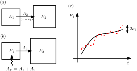
Figure 1: The energy fluctuations in the two set-ups. (a) Exchange of energy between two systems. (b) A system driven by an external force and attached to a bath. (c) A typical evolution of $E_{1}\left(t\right)$ (dashed line) fluctuates around the average $\left\langle E_{1}\right\rangle\left(t\right)$ (solid line). Eq. (7) relates the size of these fluctuations to the average $\left\langle E_{1}\right\rangle\left(t\right)$.

As the dynamics of a system are affected by the detailed microscopic state, repeating the same experiment will lead to different outcomes. Specifically, a measurement of the energy as a function of time will yield different results, see Fig. 1(c). The variations between experiments might average-out in large, thermodynamic systems, or when the driving protocol applied is quasi-static. However, they can be significant when the drive is not quasi-static and in small or mesoscopic systems, which are of current experimental interest cold_atoms ; trapped_ions ; nuc_spins . Here we quantify these energy fluctuations by studying the variance of the energy measurements in repeated experiments. The dependence of these fluctuations on the dynamics makes general statements scarce, and one typically has to resort to the study of specific models.

In this Letter we show that when the changes in energy are small and slow (but still irreversible), general statements about the energy fluctuations can be made. The results are insensitive to almost all microscopic details of the systems, depending only on the average energy flows from the drive to the system and between the systems as a function of time, and on the density of states. We stress that the assumptions made do not imply that the combined system (composed of systems 1 and 2) is close to equilibrium, but only that each of the systems separately is close to equilibrium within its energy shell. Our main results are: (1) Eqs. (6) and (7), which quantify the variance of the energy fluctuations as the system approaches its steady-state (which is equilibrium when no drive is present). (2) Eq. (9), which relates three main quantities at the steady-state: the variance of the energy fluctuations, the average rate of energy flow through the system, and the relaxation time of energy fluctuations. The validity of the results is illustrated in a system of colliding hard spheres.

To derive them we consider the evolution of the energies in the $\left(E_{1},E_{2}\right)$ plane, where $E_{1},E_{2}$ are the energies of systems 1 and 2 respectively. Consider a series of small changes in the energies, each taking place over a time interval $\Delta t$. We assume that $\tau_{R}\ll\Delta t$, where $\tau_{R}$ is the relaxation time of each of the isolated systems separately. When this time scale separation holds, the statistics of the energy changes $\Delta E_{1},\Delta E_{2}$ during the time interval from $t$ to $t+\Delta t$ depend only on the energies $\left(E_{1},E_{2}\right)$ at time $t$. The time evolution of the probability distribution $P_{12}\left(E_{1},E_{2}\right)$ is then governed by a Fokker-Planck equation

$$\partial_{t}P_{12}=-\sum_{i=1}^{2}\partial_{E_{i}}\left(A_{i}P_{12}\right)+\frac{1}{2}\sum_{i,j=1}^{2}\partial_{E_{i}}\partial_{E_{j}}\left(B_{ij}P_{12}\right)$$ (1)

where $A_{1},A_{2},B_{11},B_{12},B_{21},B_{22}$ are all functions of $\left(E_{1},E_{2}\right)\,$, and $B_{12}=B_{21}$. These function are related to the first two moments of the changes in $E_{1},E_{2}$ during a short time $\Delta t$ gardiner ; cumulant_comment :

$$A_{i}=\frac{\left\langle\Delta E_{i}\right\rangle}{\Delta t}\ ;\ B_{ij}=\frac{\left\langle\Delta E_{i}\Delta E_{j}\right\rangle}{\Delta t}\ .$$

The equation is valid when higher cumulants, e.g. $\left\langle\Delta E_{i}\Delta E_{j}\Delta E_{k}\right\rangle_{c}/\Delta t$, are small compared to the $A_{i}$ and $B_{ij}$ functions.

In both scenarios, of equilibrating systems and driven-dissipative systems, one can take the $A_{i}$ and $B_{ij}$ functions to depend on $E_{1}$ only. For equilibrating systems, this is possible when the initial total energy $E_{total}=E_{1}+E_{2}$ is fixed, so that $E_{2}$ can be considered to be a function of $E_{1}$. In the case of driven-dissipative systems, $E_{2}$ drops completely from the equations when we take system 2 to be much larger than system 1. As shown below, this is because system 2 acts as a thermal bath whose properties are insensitive to the changes in $E_{2}$. It is then more convenient to work with the marginal probability distribution of $E_{1}$ alone: $P\left(E_{1}\right)\equiv\int dE_{2}P_{12}\left(E_{1},E_{2}\right)$. Integrating Eq. (1) over $E_{2}$ we find

$$\partial_{t}P=-\partial_{E_{1}}\left(A_{1}P\right)+\frac{1}{2}\partial_{E_{1}}^{2}\left(B_{11}P\right)\ ,$$ (2)

using $P_{12}\left(E_{2}\rightarrow\pm\infty\right)=0$.  While only the functions $A_{1}$ and $B_{11}$ appear in this equation, the interaction with system 2 still affects the energy of system 1, via the forms of the functions $A_{1},B_{11}$. This is contained in the relation which is derived below

$$2A_{1}-2\beta_{2}/\beta_{1}A_{F}=\left(\beta_{1}-\beta_{2}\right)B_{11}\ ,$$ (3)

where $A_{F}\equiv A_{1}+A_{2}=\partial_{t}\left\langle E_{total}\right\rangle$ is the rate of energy injected into the system by the drive. The inverse temperatures are defined by $\beta_{1}\left(E_{1}\right)=\partial_{E_{1}}S_{1}\left(E_{1}\right)$, and $\beta_{2}\left(E_{2}\right)=\partial_{E_{2}}S_{2}\left(E_{2}\right)$, where $S_{1,2}$ are the (microcanonical) entropies of systems 1,2 respectively. $\beta_{1}$ and $\beta_{2}$ are well-defined functions, depending only on the density of states of the system, and unrelated to the driving mechanism and the interaction between the systems. Moreover, $\beta_{1}$ can be very different from $\beta_{2}$. Eq. (3) is ultimately based on Liouville’s equation, or the unitarity of the dynamics in quantum cases. In the driven case we also assume that the energy flow from the drive and between the systems are statistically independent processes, see discussion below. Eq. (3) is exact up to corrections of order $1/N$, where $N$ is the number of degrees of freedom of the smaller of the two systems. In the case of equilibrating systems $A_{F}=0$, and the relation Eq. (3) reduces to $2A_{1}=\left(\beta_{1}-\beta_{2}\right)B_{11}$. Here, as expected, on average energy flows from high to low temperatures.

The drive is implemented by varying the Hamiltonian of system 1 in time (e.g., by applying a time-varying external field). We consider drives where the Hamiltonian repeatedly returns to its original form (i.e., an oscillating field). At the steady-state, when the Hamiltonian is changed adiabatically, returning to the original form leaves the energy of the combined system unchanged. Thus, the changes in the energy will only be due to irreversible effects.

Before deriving Eq. (3) we consider several of its consequences in the two scenarios, of equilibrating and driven-dissipative systems. Wherever possible, we present the results in a unified way where the case of equilibrating systems is obtained by setting $A_{F}=0$.

Approach to steady-state - We start by considering the approach of the combined system (composed of systems 1 and 2) to its steady-state. If no driving is present (scenario 1), this steady-state is thermal equilibrium. We derive an expression for the evolution of the variance $\sigma_{1}^{2}=\left\langle E_{1}^{2}\right\rangle-\left\langle E_{1}\right\rangle^{2}$ during the entire equilibration process. Proceeding similarly to NatPhys , we take the first two moments with respect to $E_{1}$ of Eq. (2)

$$\partial_{t}\left\langle E_{1}\right\rangle =\left\langle A_{1}\right\rangle\ ,$$

$$\partial_{t}\sigma_{1}^{2} =\left\langle B_{11}\right\rangle+2\left(\left\langle A_{1}E_{1}\right\rangle-\left\langle A_{1}\right\rangle\left\langle E_{1}\right\rangle\right)\ .$$ (4)

If the distribution is narrow enough (valid up to $1/N$ corrections, see discussion after Eq. (7)), $\left\langle A_{1}\right\rangle$ can be assumed to depend on $\left\langle E_{1}\right\rangle$ alone, and the change in $\left\langle E_{1}\right\rangle$ will be monotonic. Combining the two equalities in Eq. (4) and linearizing $A_{1}$ within the width of the probability distribution, we find

$$\frac{\partial\sigma_{1}^{2}}{\partial\left\langle E_{1}\right\rangle}=2Z\left(\left\langle E_{1}\right\rangle\right)+2\frac{\partial_{E_{1}}A_{1}\left(\,\left\langle E_{1}\right\rangle\right)}{\left\langle A_{1}\right\rangle}\sigma_{1}^{2}\left(\left\langle E_{1}\right\rangle\right)\ ,$$ (5)

where $Z\left(\left\langle E_{1}\right\rangle\right)\equiv B_{11}/\left(2A_{1}\right)$. Solving the ordinary differential equation Eq. (5) and using Eq. (3) we find for the equilibrating systems that the variance is given by

$$\sigma_{1,eq}^{2}\left(\left\langle E_{1}\right\rangle\right)= \sigma_{1_{0}}^{2}\frac{A_{1}^{2}\left(\left\langle E_{1}\right\rangle\right)}{A_{1}^{2}\left(\left\langle E_{1}\right\rangle_{0}\right)}+$$

$$2A_{1}^{2}\left(\left\langle E_{1}\right\rangle\right)\int_{\left\langle E_{1}\right\rangle_{0}}^{\left\langle E_{1}\right\rangle}\frac{1}{A_{1}^{2}\left(E^{\prime}\right)\left(\beta_{1}-\beta_{2}\right)}dE^{\prime}\ .$$ (6)

Here $\left\langle E_{1}\right\rangle_{0}$ and $\sigma_{1_{0}}^{2}$ are $\left\langle E_{1}\right\rangle$ and $\sigma_{1}^{2}$ respectively at the initial time. Recall that $E_{total}$ is held constant in this expression. It is easy to extend these results when $E_{total}$ varies between experiments. It is interesting to note that this expression is identical to that obtained for a single driven isolated system NatPhys when $\beta_{2}$ is set to zero. This means that within this theory, driving a system is formally equivalent to attaching it to a bath with infinite temperature. It is straightforward to show, that when system 2 is a bath, so that $\beta_{2}$ can be taken to be a constant, the width $\sigma_{1}^{2}$ approaches the equilibrium value: $\left(\partial_{E_{1}}\beta_{1}\right)_{E_{eq}}^{-1}=k_{B}T^{2}C$, were $E_{eq}$ is the equilibrium value of $\left\langle E_{1}\right\rangle$, and $C$ is the heat-capacity (see e.g., kardar ). To see this, note that at equilibrium $A_{1}$ must vanish, and $\beta_{1}=\beta_{2}$. Therefore the entire expression for $\sigma_{1}^{2}$ is controlled by the final approach of $E$ to $E_{eq}$ where

$$\beta_{1} \simeq\beta_{2}+\left(\partial_{E_{1}}\beta_{2}\right)_{E_{eq}}\left(E-E_{eq}\right)\ ,$$

$$A_{1}\left(E^{\prime}\right) =\left.\frac{dA_{1}}{dE_{1}}\right|_{E_{eq}}\left(E-E_{eq}\right)\ ,$$

and the equilibrium expression follows. Note that away from the final equilibration regime $A_{1}\left(E\right)$ need not be linear.

In the case of driven-dissipative systems (when system 2 is large), we obtain for the variance

$$\sigma_{1,dd}^{2}\left(\left\langle E_{1}\right\rangle\right)=\sigma_{1_{0}}^{2}\frac{A_{1}^{2}\left(\left\langle E_{1}\right\rangle\right)}{A_{1}^{2}\left(E_{1_{0}}\right)}+2A_{1}^{2}\left(\left\langle E_{1}\right\rangle\right)\int_{E_{1_{0}}}^{\left\langle E_{1}\right\rangle}\frac{Z\left(E^{\prime}\right)}{A_{1}^{2}\left(E^{\prime}\right)}dE^{\prime}\ .$$ (7)

where $Z=\left[1-\beta_{2}A_{F}/\left(\beta_{1}A_{1}\right)\right]/\left(\beta_{1}-\beta_{2}\right)$. Eqs. (6) and (7) are our main results for the approach to steady-state. They predict the size of fluctuations in $E_{1}$ around its average value. They depend only on the rates of energy injection into the system $A_{F}$ (which is zero for equilibrating systems) and the rate of energy transfer to the bath $A_{2}$. In principle both these quantities can be measured separately. $A_{F}$ can be measured by the rate of energy absorption when system 1 is isolated, and $A_{2}$ in an equilibration experiment without the drive. This is a consequence of our assumption of statistical independence of the driving and the mechanism of interaction between the systems. In addition we comment that Eqs. (6) and (7) imply that $\sigma_{1,eq}^{2}$ and $\sigma_{1,dd}^{2}$ scale as $E\propto N$ when $A$ is a homogeneous function of $N$ (e.g., extensive in $N$). This justifies self-consistently our assumption on the narrowness of the distribution.

Steady-state fluctuations - The framework described above can also be used to study fluctuations in the steady-state of driven-dissipative systems, specifically fluctuations of $E_{1}$ around $\left\langle E_{1}\right\rangle$. At the steady-state the probability distribution $P_{s}\left(E_{1}\right)$ is independent of time. Using $\partial_{t}\left\langle E_{1}\right\rangle=\left\langle A\right\rangle=A\left(\left\langle E_{1}\right\rangle\right)$, and noting that at the steady-state $A\left(\left\langle E_{1}\right\rangle\right)$ must vanish, we expand $A_{1}$ and $B_{11}$ to lowest order in $e_{1}\equiv E_{1}-E_{1}^{0}$

$$A_{1}=-\frac{1}{\tau}e_{1}\ ,\ \ \ B_{11}=B_{s}$$ (8)

where $B_{s}$ and $\tau$ are constants. Equivalently, in this regime the Fokker-Planck equation describes the Brownian motion of the energy in a harmonic potential $\dot{e}_{1}=-e_{1}/\tau+\sqrt{B_{s}}\eta$, where the white noise $\eta\left(t\right)$ satisfies $\left\langle\eta\left(t\right)\eta\left(t^{\prime}\right)\right\rangle=\delta\left(t-t^{\prime}\right)$. $\tau$ is then interpreted as the relaxation time, as can be seen from the two time correlation function

$$\left\langle e_{1}\left(t_{1}\right)e_{1}\left(t_{2}\right)\right\rangle=\frac{B_{s}\tau}{2}e^{-\left|t_{2}-t_{1}\right|/\tau}\ .$$

The variance of the energy fluctuations is given by $\sigma_{1}^{2}=\left\langle e_{1}\left(t_{1}\right)^{2}\right\rangle=B_{s}\tau/2$.

When $A_{F}=0$, Eqs. (3) and (8) imply that$\ e_{1}=-\frac{\tau B_{s}}{2}\left(\beta_{1}-\beta_{2}\right)$. Then expanding $\beta_{1}$ around $\beta_{2}$ as done above we find that $\sigma_{1}^{2}=B_{s}\tau/2=-\left(\partial_{E_{1}^{0}}\beta_{1}\right)^{-1}$ which again reproduces the canonical distribution width. The present derivation gives a dynamic interpretation to this formula.

When $A_{F}\neq 0$ namely for a driven-dissipative system we find, using $A_{1}\left(E_{1}^{0}\right)=0$ in Eq. (3), and $\sigma_{1}^{2}=B_{s}\tau/2$, that

$$\tau A_{F}=\frac{\beta_{1}}{\beta_{2}}\left(\beta_{2}-\beta_{1}\right)\sigma_{1}^{2}\ .$$ (9)

This is our main result for the steady-state of driven-dissipative systems. $A_{F}$ is the rate of energy injected to the system from the drive. In the steady-state, this energy is then dissipated into the bath. This expression therefore relates three central quantities characterizing the steady-state: the size of the energy fluctuations $\sigma_{1}^{2}$, the rate of energy dissipation $A_{F}$, and $\tau$ which is the relaxation time in the steady-state 2_baths_comment .

MD Simulations - Before proving the key relation Eq. (3), we illustrate our main results on a gas of hard-sphere particles in a box, simulated by an event-driven molecular dynamics simulation MDbook . The gas is composed of $N_{1}$ particles of mass $m_{1}$ and $N_{2}$ particles of mass $m_{2}$, all of equal size, corresponding to systems 1 and 2 respectively. Although the entropy of the two systems between collisions indeed factorizes, the collision process involves a strong interaction, which changes the velocities of the particles by a significant amount. A collision calculation shows that if the two masses are very different, the energy transfer in each collision is small. In this case energy transfer occurs over many collisions, fulfilling the assumption of time-scale separation (see above). In what follows we take $m_{1}=10^{-4}$, $m_{2}=1$. (Throughout we use arbitrary units). The box is a unit cube with reflecting boundary-conditions, and the particles are taken to occupy a volume fraction of $0.05$.

We first consider the approach to equilibrium of two systems in contact, Fig. 1(a), to be compared with the predictions of Eq. (6). We take $N_{1}=30$ for the first systems and $N_{2}=20$ for the second system. $N_{1},N_{2}$ are chosen to be relatively small in order to test the theory on a mesoscopic system. The initial velocities are sampled from a Maxwell-Boltzmann distribution with $\beta_{1}=60$ and $\beta_{2}=3$, corresponding to average energies per particle of $\left\langle E_{1}\right\rangle/N_{1}=0.025$ and $\left\langle E_{2}\right\rangle/N_{2}=0.5$. We start all runs from a fixed total energy $E_{total}=\left\langle E_{1}\right\rangle+\left\langle E_{2}\right\rangle$, by preforming a (small) rescaling of the $m_{2}$-particles’ velocities. Gathering statistics over many runs, we calculate at each time the average energy $\left\langle E_{1}\right\rangle\left(t\right)$ and the variance $\sigma_{1}^{2}\left(t\right)$. The function $A_{1}\left(\left\langle E_{1}\right\rangle\right)$ is obtained by plotting $A_{1}\left(t\right)=d\left\langle E_{1}\right\rangle/dt$ as a function of $\left\langle E_{1}\right\rangle\left(t\right)$. Given $A_{1}\left(\left\langle E_{1}\right\rangle\right)$ Max_model_comment  we use Eq. (6) to predict $\sigma_{1}^{2}\left(\left\langle E_{1}\right\rangle\right)$, and find a good fit with the simulation results, see Fig. 2.

Figure 2: Equilibration of a system of 50 particles with two different masses. Plotted are simulation results for $\left\langle E_{1}\right\rangle$ vs. $\sigma_{1}^{2}$ (dots) compared to the theoretical prediction (solid line), Eq. (6). Inset: Example of $E_{1}\left(t\right)$ in a single run (solid line), and the average energy $\left\langle E_{1}\right\rangle\left(t\right)$ (dashed line), used to calculate $A_{1}$.

We now turn to the driven-dissipative scenario, and test Eq. (9) for the steady-state. We run simulations on a system with $N_{1}=10$ and $N_{2}=50$ particles. System 1 is driven by applying short impulses to the $m_{1}$-particles, changing their velocity by $\Delta\mathbf{v}=\mathbf{F}\delta t/m_{1}$, where $\mathbf{F}$ is a constant force and $\delta t$ the impulse duration. This impulse is applied at a constant rate. In order to mimic the behavior of a very large system 2, the velocity of the $m_{2}$ particles is changed upon reflection from the wall MD_BCs , so as to maintain a constant $\left\langle E_{2}\right\rangle$. The quantities $\tau,A_{F},\beta_{1}$ and $\sigma_{1}^{2}$ are computed from the numerics. The energy of system 2 is maintained at $\left\langle E_{2}\right\rangle/N_{2}=1/2$, or $\beta_{M}=3$. Fig. 3 shows the results obtained for the two sides of Eq. (9) as a function of $\beta_{1}/\beta_{2}$ for different strengths of the drive. Good agreement is found over a wide range of drive strengths, and temperature differences. In this range, $A_{F}$ increases by a factor of 1000, $\sigma_{1}^{2}$ by a factor of 17, and the relaxation time $\tau$ decreases by a factor of 3.

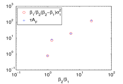
Figure 3: Test of Eq. (9) for a driven-dissipative system. .

Derivation of the eq. (3) - We end by deriving Eq. (3). To do so we look at two times $t,t+\Delta t$ in which the driving protocol has returned to its original state, i.e. where $H\left(t\right)=H\left(t+\Delta t\right)$, where $H$ is the Hamiltonian of the combined system. As stated before, we assume that both subsystems are relaxed in their respective energy shells, with energies $E_{1}$ and $E_{2}$. In particular, this requires that $\Delta t\gg\tau_{R}$. We denote the changes in $E_{1},E_{2}$ during the time interval $\Delta t$ by $\Delta E_{1},\Delta E_{2}$ respectively, and define $\Delta E_{B}$ and $\Delta E_{F}$ via

$$\Delta E_{1}=\Delta E_{F}-\Delta E_{B}\ ,\ \Delta E_{2}=\Delta E_{B}\ .$$

$\Delta E_{B}$ is the energy transferred from system 1 to system 2, and $\Delta E_{F}$ is the work done on system 1 by the external drive.

Under these assumptions, Liouville’s theorem or the unitarity of the dynamics, together with micro-reversibility of the dynamics, imply a Crooks relation for the combined isolated system crooks ; isolated_crooks ; QM_crooks

$$P_{E_{1},E_{2}}\left(\Delta E_{1},\Delta E_{2}\right)e^{S_{1}\left(E_{1}\right)+S_{2}\left(E_{2}\right)}$$

$$=\tilde{P}_{E_{1}+\Delta E_{1},E_{2}+\Delta E_{2}}\left(-\Delta E_{1},-\Delta E_{2}\right)e^{S_{1}\left(E_{1}+\Delta E_{1}\right)+S_{2}\left(E_{2}+\Delta E_{2}\right)}\ ,$$

where $P_{E_{1},E_{2}}\left(\Delta E_{1},\Delta E_{2}\right)$ is the probability of a transition $\left(E_{1},E_{2}\right)\rightarrow\left(E_{1}+\Delta E_{1},E_{2}+\Delta E_{2}\right)$, and $\tilde{P}$ is defined similarly, only with respect to the the reversed protocol, defined by the dynamics generated by the time-reversed Hamiltonian, $\tilde{H}\left(t^{\prime}\right)=H\left(t+\Delta t-t^{\prime}\right)$.

We assume that: (1) $\Delta E_{1},\Delta E_{2}$ are small so that the transition probabilities depend weakly on the initial energies $\tilde{P}_{E_{1}+\Delta E_{1},E_{2}+\Delta E_{2}}=\tilde{P}_{E_{1},E_{2}}$, with corrections which are of order $N^{-1}$ NatPhys . (2) $\Delta E_{B}$ and $\Delta E_{F}$ are statistically independent quantities. This happens when the interaction with the bath is independent from the driving process, e.g., when the drive and interaction processes act on different modes, on different parts of the system, at different times, etc.. These imply that

$$P^{F}\left(\Delta E_{F},0\right)P^{B}\left(-\Delta E_{B},\Delta E_{B}\right)e^{-\beta_{1}\delta E_{F}-\left(\beta_{2}-\beta_{1}\right)\delta E_{B}}$$

$$=\tilde{P}^{F}\left(\Delta E_{F},0\right)\tilde{P}^{B}\left(-\Delta E_{B},\Delta E_{B}\right)\ .$$

Integrating over $\Delta E_{F},\Delta E_{B}$ gives a Jarzynski relation $\left\langle e^{-\beta_{1}\Delta E_{F}}\right\rangle\left\langle e^{-\left(\beta_{2}-\beta_{1}\right)\Delta E_{B}}\right\rangle=1$. Rearranging the equation and again integrating gives $\left\langle e^{-\beta_{1}\Delta E_{F}}\right\rangle=\left\langle e^{-\left(\beta_{2}-\beta_{1}\right)\Delta E_{B}}\right\rangle$ yielding $\left\langle e^{-\beta_{1}\Delta E_{F}}\right\rangle=\left\langle e^{-\left(\beta_{2}-\beta_{1}\right)\Delta E_{B}}\right\rangle=1$. The second relation is the exchange fluctuation relation fluct_heat_exchange ; QM_fluct_relation_review ; The first is a variant of the Jarzynski relation for isolated systems NatPhys . Expanding both to second order we find

$$2\left\langle\Delta E_{F}\right\rangle=\beta_{1}\left\langle\Delta E_{F}^{2}\right\rangle\ ,\ 2\left\langle\Delta E_{B}\right\rangle=\left(\beta_{2}-\beta_{1}\right)\left\langle\Delta E_{B}^{2}\right\rangle\ .$$

From independence it follows that $\left\langle\Delta E_{F}\Delta E_{1}\right\rangle=\left\langle\Delta E_{F}^{2}\right\rangle$, or $\left\langle\Delta E_{B}^{2}\right\rangle=\left\langle\Delta E_{1}^{2}\right\rangle-\left\langle\Delta E_{F}^{2}\right\rangle$. The second equation becomes $2\left\langle\Delta E_{B}\right\rangle=\left(\beta_{2}-\beta_{1}\right)\left(\left\langle\Delta E_{1}^{2}\right\rangle-\left\langle\Delta E_{F}^{2}\right\rangle\right)$, so that

$$2\left\langle\Delta E_{1}\right\rangle-2\beta_{2}/\beta_{1}\left\langle\Delta E_{F}\right\rangle=\left(\beta_{1}-\beta_{2}\right)\left\langle\Delta E_{1}^{2}\right\rangle\ .$$

After dividing by $\Delta t$ and using the definitions of the $A_{i},B_{i}$ quantities, yields Eq. (3).

Acknowledgments - We are grateful to Luca D’Alessio, Dov Levine, Daniel Podolsky and Anatoli Polkovnikov for many useful discussions and comments. The work was supported by a BSF grant. YK thanks G. M. Schutz.

References

(1)Granular Gas Dynamics, edited by T. P¨oschel and N. Brilliantov (Springer, Berlin, 2003)
(2)Y. Srebro and D. Levine, Phys. Rev. Lett. 93, 240601 (2004)
(3) E. G. Dalla Torre, E. Demler, T. Giamarchi and E. Altman,
Nature Physics 6, 806–810 (2010)
(4)I. Bloch, J. Dalibard, W. Zwerger, Rev. Mod. Phys. 80,
885-964 (2008)
(5)R. Blatt and D. J. Wineland, Nature 453, 1008-1015 (2008)
(6)J.R. Petta, J. M. Taylor, A. C. Johnson, A. Yacoby, M. D.
Lukin, C. M. Marcus, M. P. Hanson, and A. C. Gossard, Phys. Rev. Lett. 100,
067601-067604 (2008)
(7)C. W. Gardiner, Handbook of stochastic methods for physics,
chemistry, and the natural sciences, Springer (1994)
(8)For finite one should in principle
consider cumulents. Here, as is short, the distinction disappears.
(9)G. Bunin, L. D’Alessio, Y. Kafri and A. Polkovnikov, Nature
Phys. 7, 913–917 (2011)
(10)M. Kardar, Statistical Physics of Particles, Cambridge
University Press (2007)
(11)A similar derivation can be carried out for a system
coupled to two baths at temperatures and , instead of
one bath and a drive. One then obtains the for the steady-state .
(12)M. P. Allen and D. J. Tildesley, Computer simulation of
liquids, Oxford University Press (1989)
(13)Incidentally, is found to fit very well to a function of the form
, or ,
allowing us to write a closed analytical expression for . This can be understood by calculating
the rate of energy transfer, taking the collision rate to depend only on the
velocity of the lighter, and hence faster, particles.
(14)J. L. Lebowitz and H. Spohn, J. Stat. Phys, 19, 6 (1978)
(15)G. E. Crooks, J. Stat. Phys. 90, 1481-1487 (1998)
(16)P. Pradhan, Y. Kafri, and D. Levine, Phys. Rev E 77,
041129-041135 (2008)
(17)In the quantum mechanical setting we assume that the
initial and final density matrices are diagonal, as in NatPhys , and
that there is no significant entangelment between the two systems.
(18)C. Jarzynski and Daniel K. Wójcik, Phys.
Rev. Lett. 92, 230602 (2004)
(19)M. Campisi, P. Hanggi and P. Talkner, Rev.
Mod. Phys. 83, 771–791 (2011)