Efficient Algorithms for Solving Hypergraphic Steiner Tree Relaxations in Quasi-Bipartite Instances

Abstract

We consider the Steiner tree problem in quasi-bipartite graphs, where no two Steiner vertices are connected by an edge. For this class of instances, we present an efficient algorithm to exactly solve the so called directed component relaxation (DCR), a specific form of hypergraphic LP relaxation that was instrumental in the recent break-through result by Byrka et al. [2]. Our algorithm hinges on an efficiently computable map from extreme points of the bidirected cut relaxation to feasible solutions of (DCR). As a consequence, together with [2] we immediately obtain an efficient 73/60-approximation for quasi-bipartite Steiner tree instances. We also present a particularly simple (BCR)-based random sampling algorithm that achieves a performance guarantee slightly better than 77/60.

1 Introduction

In the Steiner tree problem, we are given an undirected graph $G=(V,E)$ with costs $c$ on edges and its vertex set partitioned into terminals (denoted $R\subseteq V$) and Steiner vertices ($V\setminus R$). A Steiner tree is a tree spanning all of $R$ plus any subset of $V\subseteq R$, and the problem is to find a minimum-cost such tree. The Steiner tree problem is $\mathsf{APX}$-hard, thus the best we can hope for is a constant-factor approximation algorithm. In particular, the best inapproximability known (assuming $\mathsf{P}\not=\mathsf{NP}$) is 1.01063 ($>\frac{96}{95}$) due to Chlebík and Chlebíková [6]. For the special family of instances that are known as quasi-bipartite graphs, which is the subject of our work, the best hardness known is 1.00791 ($>\frac{128}{127}$) [6], under the same complexity assumption.

In a recent break-through paper, Byrka, Grandoni, Rothvoß and Sanità [2, 3] presented the currently best approximation algorithm known for the problem. The algorithm has a performance ratio of $\ln(4)+\epsilon$ for any fixed $\epsilon>0$, and it iteratively rounds solutions to a so called hypergraphic linear program. Such LPs commonly have a variable $x_{K}$ for each $K\subset R$, representing a full component spanning the terminals of $K$. A full component is a tree whose leaves are terminals and whose internal vertices are non-terminals.

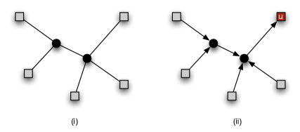
Figure 1: Example of a full components and a directed full component.

Figure 1.(i) shows an example of a full component spanning a set of terminals (squares). There are several equivalent hypergraphic LPs [4]; here we focus on the directed component relaxation (DCR) that was first introduced by Polzin and Vahdati Daneshmand [10], and then later used by Byrka et al. [2, 3]. We will now describe this LP.

Given a full component $K$ and one of its terminals $u$, we obtain a directed full component by orienting all of $K$’s edges towards the sink node $u$. Vertices $v\in K\setminus u$ are called sources; an illustration is given in Figure 1.(ii). Note that when there are no Steiner-Steiner edges, i.e. when the instance is quasi-bipartite, then every full component is associated with only one Steiner vertex which we call the centre of the full component.

In the following, we let $\mathcal{K}$ denote the set of all directed full components, and for $K\in\mathcal{K}$, we let $\operatorname{sink}$(K) be the sink node of $K$. We will sometimes abuse notation, and use $K\in\mathcal{K}$ for the set of arcs of the corresponding oriented full component, and for the set of terminals it spans interchangeably. We use $c_{K}$ for the cost of the full component $K$. For a set $U\subseteq R$, we let $\Delta^{+}(U)$ denote the set of components $K\in\mathcal{K}$ whose sink lies outside $U$ and that have at least one source in $U$. In this case, we will also say that $K$ crosses $U$. We also use $x(S)$ as a short for $\sum_{j\in S}x_{j}$. (DCR) has a variable for every $K\in\mathcal{K}$, and a constraint for every set $U\subseteq R\setminus r$, where $r\in R$ is an arbitrarily chosen root node. In the following we say that $U\subseteq V$ is valid if it contains at least one terminal, but not the root.

$$\min\quad \sum_{K\in\mathcal{K}}c_{K}x_{K}$$ (DCR)

s.t. $$x(\Delta^{+}(U))\geq 1\quad\forall U\subseteq R$$

$$x\geq 0$$

$$\min\quad \sum_{a\in A}c_{a}x_{a}$$ (BCR)

s.t. $$x(\delta^{+}(U))\geq 1\quad\forall\mbox{ valid }U\subseteq V$$

$$x\geq 0$$

Goemans et al. [8] recently showed that solving (DCR) is strongly NP-hard. Nevertheless, for any fixed $\epsilon$ there exist an efficient $(1+\epsilon)$-approximation for the value of (DCR) in the following sense: Let $(\mbox{DCR}(k)$) be the version of (DCR) that omits variables for full components with more than $k$ terminals. Borchers and Du [1] showed that the optimum value of $(\mbox{DCR}(k)$) is larger than that of (DCR) by at most a factor $\rho_{k}$ where

$$\rho_{k}=\frac{(t+1)2^{t}+s}{t2^{t}+s},$$

where we let $t\in\mathbb{N}$ and $s<2^{t}$ such that $k=2^{t}+s$. Byrka et al. [2, 3] compute such an approximate solution of (DCR), and the performance guarantee of their algorithm is $\rho_{k}\cdot\ln 4$; for every $\epsilon$, the value $k$ can be chosen large enough such that this is at most $\ln(4)+\epsilon$. One easily sees that already for moderately small values of $\epsilon$, large values of $k$ need to be chosen. E.g., for $\rho_{k}\cdot\ln 4$ to be smaller than $1.6$, we need $k$ to be bigger than $90$ (compare this to $\ln 4\leq 1.39$). For such values of $k$, solving $(\mbox{DCR}(k)$) becomes a challenge since even compact reformulations of $(\mbox{DCR}(k)$) [2, 3] have $O(n^{k})$ variables, and equally many constraints.

In this paper, we study the bidirected cut relaxation (BCR)  [7]. In this relaxation, we convert first the original instance $G=(V,E)$ into the digraph $D=(V,A)$, where $A$ has arcs $(u,v)$ and $(v,u)$ for every edge $uv\in E$; both arcs have the same cost as $uv$. We once again pick an arbitrary root terminal $r\in R$, and call a set $U\subseteq V$ valid if it contains terminals but not the root. (BCR) has a variable for every arc in $A$, and a constraint for every valid set.

Despite the fact that this relaxation is widely considered to be strong, its integrality gap is only known to be at least $36/31$ [3], and at most $2$. The known lower and upper bounds on the integrality gap of (DCR), on the other hand, are $8/7$ [9] and $\ln(4)$ [8].

In this note we focus on the class of quasi-bipartite Steiner tree instances – instances, where no two Steiner nodes are connected by an edge. Our main result for such instances with $n$ many vertices and $m$ many edges is the following.

Theorem 1.

For quasi-bipartite Steiner tree instances, (DCR) can be solved exactly using $O(mn^{3})$ minimum $s,t$-cut computations in graphs with $O(mn)$ vertices.

We accomplish this by solving (BCR), and by giving an efficient decomposition algorithm that maps the given minimal (BCR) solution to one of (DCR). We note that Chakrabarty et al. [4] had previously shown that (BCR) and (DCR) have the same optimal values in quasi-bipartite graphs. The proof in [4] uses “dual” arguments, however, and it is not clear how to obtain a “primal” algorithm.

The above theorem has a couple of consequences. First, we can use it together with [2, 3] to obtain an efficient $73/60$-approximation for quasi-bipartite Steiner tree instances. We also obtain a slightly weaker $1.28$-approximation that uses a particularly simple sampling strategy based on (BCR).

We remark that Goemans et al. [8] have recently obtained an alternative proof of Theorem 1. The work presented here was obtained before [8] appeared on the arXiv, and is therefore independent.

2 Decomposing (BCR) extreme points

In this section we provide a proof of Theorem 1. In the following fix a quasi-bipartite instance of the Steiner tree problem. Let $G=(V,E)$ be the input graph, $R\subseteq V$ the set of terminals, and $c_{e}$ a non-negative cost for each of the edges $e\in E$. Also let $D=(V,A)$ be the digraph obtained from $G$ by replacing each edge $e=uv$ by two arcs $(u,v)$, and $(v,u)$ each having cost $c_{e}$. We choose a fixed root node $r\in R$, and call a set $U\subseteq V$ valid if it contains some terminals, but not the root.

Let $y$ be a feasible solution for (DCR). We define the following natural map from the space $\mathbb{R}^{\mathcal{K}}$ to $\mathbb{R}^{A}$:

$$\Phi(y)=\sum_{K}\chi_{K}\cdot y_{K},$$

where $\chi_{K}$ is the characteristic vector of the arcs of full component $K$. The proof of the following observation is straight forward, and makes use of the fact that a full component crosses a valid set $U$ only if at least one of its arcs does.

Observation 2.

If $y$ is feasible for (DCR) then $\Phi(y)$ is feasible for (BCR).

Notice that $\Phi$ is cost-preserving, and it therefore follows immediately that the optimum solution value of (BCR) is at most that of (DCR). In order to prove Theorem 1 it suffices to show that, in the case of quasi-bipartite graphs, the optimum of (DCR) is at most the optimum of (BCR) as well. We accomplish this by showing that, given a minimal solution $x$ of (BCR), we can efficiently find a minimal solution $y$ of (DCR) such that $\Phi(y)=x$. We start by giving an overview of the proof. We define the following polyhedron:

$$\mathcal{I}:=\left\{(x,y)\in\mathbb{R}_{+}^{A}\times\mathbb{R}_{+}^{\mathcal{K}}:x(\delta^{+}(U))+y(\Delta^{+}(U))\geq 1,\quad\forall\mbox{ valid }U\subseteq V\right\}.$$ (1)

Clearly, if $x$ is feasible for (BCR) then $(x,\textbf{0})\in\mathcal{I}$. Call a full component $K\in\mathcal{K}$ feasible with respect to $(x,y)\in\mathcal{I}$ if we can shift fractional $\lambda$-weight from the arcs of $K$ to the full component $K$. Formally, $K$ is feasible if

$$(x-\lambda\cdot\chi_{K},y+\lambda\cdot e_{K})\in\mathcal{I},$$ (2)

for some $\lambda>0$, where $e_{K}$ is the standard orthonormal vector indexed by full components in $\mathcal{K}$. Our first goal then is to show in Section 2.1 that a feasible component always exists. Then in Section 2.2 we show how to efficiently compute such a feasible component $K$, which allows us to find in Section 2.3 the maximum $\lambda$ corresponding to $K$ such that (2) holds. Our strategy then is self-evident. Starting with the initial feasible vector $(x^{0},y^{0})=(x,\textbf{0})$ to $\mathcal{I}$, we define a sequence of values $\lambda^{1},\lambda^{2},\ldots$ as above, giving rise to a sequence of feasible vectors $(x^{i},y^{i})=(x^{i-1}-\lambda^{i}\cdot\chi_{K},y^{y-i}+\lambda^{i}\cdot e_{K})$ to $\mathcal{I}$, where $K$ is the full component corresponding to the value $\lambda^{i}$. Finally, in Section 2.4 we argue that the sequence above converges in polynomial many steps into a feasible vector $(\textbf{0},y)$ to $\mathcal{I}$. Since the weight shifting at every step preserves the total cost, our main theorem follows.

We now fill in the details, and begin with a few existential results. Subsequently, we show how to obtain a strongly polynomial decomposition algorithm.

2.1 Existential results

In the following it will be convenient to study slight generalizations of (BCR) and (DCR). Let $f$ be an intersecting supermodular function defined on subsets of terminals; i.e., we have

$$f(A)+f(B)\leq f(A\cap B)+f(A\cup B),$$

for any $A,B\subseteq R$ with $A\cap B\neq\emptyset$. We then obtain the LPs (BCR_f) and (DCR_f) by replacing 1 by $f$ on the right-hand sides.

$$\min\quad \sum_{K\in\mathcal{K}}c_{K}x_{K}$$ (DCR_f)

s.t. $$x(\Delta^{+}(U))\geq f(U)\quad\forall U\subseteq R$$

$$x\geq 0$$

$$\min\quad \sum_{a\in A}c_{a}x_{a}$$ (BCR_f)

s.t. $$x(\delta^{+}(U))\geq f(U\cap R)\quad\forall\mbox{ valid }U\subseteq V$$

$$x\geq 0$$

Chakrabarty et al. [4] showed that the optimal values of (BCR) and (DCR) coincide for quasi-bipartite instances. It is an easy exercise to see that their proof extends to (BCR_f) and (DCR_f). We provide an alternate proof of this fact in the appendix.

Theorem 3.

The optimal values of (BCR_f) and (DCR_f) coincide for quasi-bipartite instances, non-negative (not necessarily symmetric) costs $c$, and intersecting supermodular function $f$.

The following is now an easy corollary.

Lemma 4.

If $G$ is quasi-bipartite, $f$ is intersecting supermodular, and $x$ is an extreme point of (BCR_f), then there exists an extreme point $y$ of (DCR_f) such that $\Phi(y)=x$.

Proof.

By the theory of linear programming, there is $c\in\mathbb{R}^{A}$ such that $x$ is the unique optimal solution of (BCR_f). Since the feasible region of (BCR_f) is upward-closed, we have $c\geq 0$, for otherwise $x$ would not be optimal. We claim next that (DCR_f) is feasible. Indeed, since (BCR_f) is feasible, we know $f(R),f(\emptyset)\leq 0$, and hence (DCR) is feasible. Any feasible solution to (DCR) can now be scaled to obtain a feasible solution to (DCR_f).

Since (DCR_f) is feasible and $c\geq\textbf{0}$, we may let $y$ be an optimal extreme point solution to (DCR_f). By Theorem 3, $c^{T}y=c^{T}x$. Let $\tilde{x}=\Phi(y)$, and observe that $c^{T}\tilde{x}=c^{T}y=c^{T}x$ since $\Phi$ preserves cost. Observation 2 applies also to (BCR_f) and (DCR_f) and shows that $\tilde{x}$ is feasible for (BCR_f). As $x$ is the unique optimal solution to (BCR_f) for costs $c$, we must have $x=\tilde{x}$, and this completes the proof. ∎

The rest of this section focuses on making the above existential proof constructive. In the following we once more abuse notation, and use $\delta^{+}(U)$ ($\Delta^{+}(U)$) as the incidence vector of arcs (full components) that cross valid set $U$; $\delta^{+}_{a}(U)$, and $\Delta^{+}_{K}(U)$ then denote the component of this vector corresponding to arc $a$ and full component $K$, respectively. We obtain the following plausible lemma.

Lemma 5.

For every $K\in\mathcal{K}$, $\Delta_{K}^{+}$ is submodular i.e. if $U,W\subseteq R$, then

$$\Delta_{K}^{+}(U)+\Delta_{K}^{+}(W)\geq\Delta_{K}^{+}(U\cap W)+\Delta_{K}^{+}(U\cup W).$$

Proof.

We proceed by case analysis. If the right-hand side is zero, the inequality is trivial. Case 1: Suppose $\Delta_{K}^{+}(U\cap W)=1$ and $\Delta_{K}^{+}(U\cup W)=0$. Then, without loss of generality, the sink of $K$ lies outside $U$. Since $K$ has a sink in $U\cap W$, in particular in $U$, this implies $\Delta_{K}^{+}(U)=1$. Case 2: Suppose $\Delta_{K}^{+}(U\cap W)=0$ and $\Delta_{K}^{+}(U\cup W)=1$. Then, without loss of generality, $K$ has a source inside $U$. Since the sink of $K$ lies outside $U\cup W$, in particular $U$, this implies $\Delta_{K}^{+}(U)=1$. Case 3: Finally, suppose $\Delta_{K}^{+}(U\cap W)=1$ and $\Delta_{K}^{+}(U\cup W)=1$. Then $K$ has a source inside $U\cap W$ and its sink lies outside both $U$ and $W$, so $\Delta_{K}^{+}(U)=\Delta_{K}^{+}(W)=1$. ∎

The following lemma shows that a (BCR) extreme point can indeed be decomposed iteratively into full components.

Lemma 6.

Let $G$ be quasi-bipartite, let $f$ be intersecting supermodular, let $x$ be a minimal feasible solution of (BCR_f)  and let $vu\in A$ be such that $v\notin R,u\in R$, and $x_{vu}>0$. Then there exists $\lambda>0$ and $K\in\mathcal{K}$ with $vu\in K$ such that

$$x^{\prime}:=x-\lambda\chi_{K}$$ (3)

is minimally feasible in (BCR${}_{f^{\prime}}$) where $f^{\prime}$ is obtained from $f$ by reducing $f(U)$ by $\lambda$ for all valid $U$ that are crossed by $K$. Moreover, for any such $\lambda$, $f^{\prime}$ is again intersecting supermodular.

Proof.

As $x$ is a minimal feasible solution to (BCR_f) we can write it as

$$x:=\sum_{i=1}^{k}\alpha_{i}x^{i},$$

where $x^{1},\ldots,x^{k}$ are (BCR_f) extreme points, $\alpha\geq\textbf{0}$, and $\textbf{1}^{T}\alpha=1$. Since $x_{vu}>0$, $x^{j}_{vu}>0$ for some $j$. By Lemma 4, for every $i$ there exit $y^{i}$ such that $\Phi(y^{i})=x^{i}$ and $y^{i}$ is feasible to (DCR_f). Let $K\in\mathcal{K}$ be any component with $vu\in K$ and $y^{j}_{K}>0$.

Clearly, $y=\sum_{i=1}^{k}\alpha_{i}y^{i}$ is a feasible point of (DCR_f). Now obtain $y^{\prime}$ by reducing the $K$th component of $y^{j}$ in the above convex combination to $0$; i.e., let

$$y^{\prime}=y-\alpha_{j}y^{j}_{K}e_{K}.$$

Let $f^{\prime}=f-\alpha_{j}y^{j}_{K}\Delta^{+}_{K}$; i.e., we obtain $f^{\prime}$ from $f$ by reducing $f(U)$ by $\alpha_{j}y^{j}_{K}$ if $K$ crosses $U$. Note that $f^{\prime}$ is intersecting supermodular as $f$ is intersecting supermodular, and $\Delta^{+}_{K}$ is submodular.

Simply from the definition of $f^{\prime}$ it now follows that $y^{\prime}$ is feasible for (DCR${}_{f^{\prime}}$), and Observation 2 shows that $x^{\prime}=\Phi(y^{\prime})$ is feasible for (BCR${}_{f^{\prime}}$). From the definitions of $\Phi$ and $y^{\prime}$ it also follows that $x^{\prime}=x-\alpha_{j}y^{j}_{K}\chi_{K}$, and we therefore choose $\lambda=\alpha_{j}y^{j}_{K}$ in (3).

Finally, suppose for the sake of contradiction that $x^{\prime}$ is not a minimal solution to (BCR${}_{f^{\prime}}$); i.e., there is an arc $a$ and $\epsilon>0$ such that $x^{\prime\prime}=x^{\prime}-\epsilon e_{a}$ is feasible for (BCR${}_{f^{\prime}}$). Then

$$x(\delta^{+}(U))-\lambda|\{a\,:\,a\in K\cap\delta^{+}(U)\}|-\epsilon\delta^{+}_{a}(U) =$$

$$x^{\prime}(\delta^{+}(U))-\epsilon\delta^{+}_{a}(U) \geq f^{\prime}(U\cap R),$$

for all valid $U\subseteq V$. Thus, we have

$$x(\delta^{+}(U))-\epsilon\delta^{+}_{a}(U)\geq f^{\prime}(U\cap R)+\lambda|\{a\,:\,a\in K\cap\delta^{+}(U)\}|,$$

for all valid $U$. Note that the right hand side of this inequality is at least $f(U\cap R)$ as $\Delta^{+}_{K}(U)\leq\chi_{K}(\delta^{+}(U))$ for all $U$. Thus, $x$ is not a minimal (BCR_f) solution, and this is the desired contradiction. ∎

2.2 Towards efficiency I : Finding feasible components

What conditions are sufficient for a full component $K$ to be feasible? Well, certainly we need $x_{a}>0$ for all $a\in K$. Beyond this, feasibility is characterized by tight valid constraints. We say that valid set $U$ is tight for $(x,y)$ if the corresponding constraint in $\mathcal{I}$ is satisfied with equality. It is easy to see that $K$ is valid iff every tight set crossed by $K$ is crossed by at most one of its arcs; i.e.,

$$\Delta^{+}_{K}(U)\geq\sum_{a\in K}\delta^{+}_{a}(U)$$ (4)

holds for all tight sets $U$. In fact, it suffices to look at certain tight sets.

Figure 2: Three classes of tight sets.

In what follows, fix a full component $K$ along with its centre $v$ and sink $u$. Figure 2.(i) shows a tight set $C$ that contains both the sink $u$ and a source terminal $w$ but not the centre $v$. In this case, the arc $(w,v)$ crosses $C$, but $K$ does not, and (4) is violated. We let $\mathcal{C}$ be the set of neighbours of $v$ that don’t lie in such a tight set, and are hence eligible source nodes:

$$\mathcal{C}=\{w\in\Gamma(v)\setminus u\,:\,\nexists\mbox{ tight valid set }U\mbox{ with }u,w\in U\mbox{ and }v\notin U\}.$$

Figure 2.(ii) shows a tight set $X$ that does not contain the centre $v$ nor the sink $u$ of $K$, but two sources $w$ and $z$. Since two of $K$’s arcs cross $X$, component $K$ is once again not feasible. A feasible component may contain at most one source from a tight set $X$ like this. We let $\mathcal{X}$ be the set of all eligible source node sets contained in such tight sets:

$$\mathcal{X}=\{X\cap\mathcal{C}\,:\,X\mbox{ is a tight valid set with }u,v\not\in X\}.$$

Finally, Figure 2.(iii) shows a set $Y$ that contains $K$’s centre but not its sink. In this case, $K$ must contain one of its sources in $Y$ as otherwise $K$ would not cross $Y$. We let $\mathcal{Y}$ be the set of all eligible source node sets contained in such tight sets:

$$\mathcal{Y}=\{Y\cap\mathcal{C}\,:\,Y\mbox{ is a tight valid set with }v\in Y,u\not\in Y\}.$$

Lemma 7.

A component $K$ with centre $v$ and sink $u$ is feasible iff (a) $x_{a}>0$ for all $a\in K$, (b) sources of $K$ lie in $\mathcal{C}$, (c) $K$ has at most one source in each set in $\mathcal{X}$, and (d) $K$ has at least one source in each set in $\mathcal{Y}$.

Proof.

If $K$ is feasible then clearly (a)-(d) above needs to be satisfied. We prove the converse.

Suppose that (a)-(d) are satisfied for some full component $K$ with centre $v$ and sink $u$. Since $x_{a}>0$ for all $a\in K$ it suffices to check that (4) holds for all tight valid sets $U$.

Consider a particular tight valid set $U$, and suppose first that $K$ crosses $U$; i.e., $K$ has its sink outside $U$, and at least one of its sources is in $U$. Then (4) is satisfied if $\delta^{+}(U)$ has at most one of $K$’s arcs. Suppose for the sake of contradiction that $\delta^{+}(U)$ has more than one arc from $K$. In this case, $v\not\in U$, and $U\cap\operatorname{sources}(K)\in\mathcal{X}$. But in this case, (b) implies that $K$ can have at most one source in $U$; a contradiction.

Now suppose that $K$ does not cross $U$, and assume for contradiction that $\delta^{+}(U)$ has some of $K$’s arcs. Assume first that $(v,u)\in\delta^{+}(U)$. In this case, $U\cap\operatorname{sources}(K)\in\mathcal{Y}$, and hence, by (d), $K$ must have a source in $U$, and therefore $K$ crosses $U$; a contradiction. Now assume that some arc $(w,v)\in K$ crosses $U$. In this case $w$ is a source of $K$, and $u$ must be in $U$ as otherwise $K$ would cross $U$. But this means that $w\not\in\mathcal{C}$, and we arrive yet again at a contradiction.

Thus, $K$ satisfies the condition in (4) for all tight sets $U$. ∎

We need the following standard uncrossing lemma.

Lemma 8.

Let $S,T\subseteq V$ be tight such that $S\cap T\cap R\not=\emptyset$. Then $S\cap T$ and $S\cup T$ are also tight valid sets.

Proof.

Since $S\cap T\cap R\not=\emptyset$, $S\cap T$ and $S\cup T$ are valid, and hence

$$\begin{array}[]{rcl}2-y(\Delta^{+}(S))-y(\Delta^{+}(T))&=&x(\delta^{+}(S))+x(\delta^{+}(T))\\ &\geq&x(\delta^{+}(S\cap T))+x(\delta^{+}(S\cup T))\\ &\geq&2-y(\Delta^{+}(S\cap T)-y(\Delta^{+}(S\cup T))\\ &\geq&2-y(\Delta^{+}(S))-y(\Delta^{+}(T)),\\ \end{array}$$

where the first inequality uses the submodularity of $x(\delta^{+}(\cdot))$, the second inequality follows from feasibility of the constraints in $\mathcal{I}$, and the last inequality uses Lemma 5. It follows that all inequalities above hold with equality. ∎

The last puzzle piece needed before we present an algorithm to find feasible components is the following structural fact.

Lemma 9.

$\mathcal{X}$ and $\mathcal{Y}$ are closed under intersection and union.

Proof.

Suppose $X_{1},X_{2}\in\mathcal{X}$ and $X_{1}\cap X_{2}\neq\emptyset$. Then, for $i\in\{1,2\}$, there is a tight valid set $U_{i}$ that does not contain $v$ and $u$, and $X_{i}=U_{i}\cap C$. Clearly, $U_{1}\cap U_{2}$ and $U_{1}\cup U_{2}$ are also valid, and they are tight by Lemma 8. Neither $U_{1}\cap U_{2}$ nor $U_{1}\cup U_{2}$ contain $u$ and $v$. Thus $U_{1}\cap U_{2}\cap\mathcal{C}=X_{1}\cap X_{2}$ and $U_{1}\cup U_{2}\cap C=X_{1}\cup X_{2}$ are also part of $\mathcal{X}$.

Similarly, if distinct $Y_{1},Y_{2}\in\mathcal{Y}$ intersect then, for $i\in\{1,2\}$, there exists a tight valid set $U_{i}$ with $u\notin U_{i}$, $v\in U_{i}$ and $Y_{i}=U_{i}\cap C$. So by Lemma 8, $U^{\prime}=U_{1}\cap U_{2}$ and $U^{\prime\prime}=U_{1}\cup U_{2}$ are tight valid sets as well. Both $U^{\prime}$ and $U^{\prime\prime}$ contain $v$ and not $u$. Therefore $U^{\prime}\cap\mathcal{C}=Y_{1}\cap Y_{2}$ and $U^{\prime\prime}\cap\mathcal{C}=Y_{1}\cup Y_{2}$ are also sets of $\mathcal{Y}$. ∎

Lemma 9 allows us to slightly refine the conditions in Lemma 7. Let us define $\mathcal{X}^{*}$ to be the set of inclusion-wise maximal sets in $\mathcal{X}$, and let $\mathcal{Y}^{*}$ be the inclusion-wise minimal elements of $\mathcal{Y}$. Then we may replace in the statement of Lemma 7 the $\mathcal{X}$ in (c) by $\mathcal{X}^{*}$, and the $\mathcal{Y}$ in (d) by $\mathcal{Y}^{*}$. Moreover, the sets $\mathcal{X}^{*},\mathcal{Y}^{*}$ along with $\mathcal{C}$ can be found in polynomial time as we explain in the next lemma.

Lemma 10.

For $(x,y)\in\mathcal{I}$, the sets $\mathcal{C},\mathcal{X}^{*},\mathcal{Y}^{*}$ can be found using $O(n)$ minimum-capacity $s,t$-cut computations.

Proof.

Let $D$ be the digraph that has node set

$$V\cup\{s\}\cup\{v_{K}\,:\,K\mbox{ full component with }y_{K}>0\}.$$

$D$ has an arc for each arc $a$ in the support of $x$; the capacity of this arc will be $x_{a}$. For each full component $K$ in the support of $y$, we add $K$’s arcs, using node $v_{K}$ instead of $K$’s real centre $v$. The sink arc $(v_{K},u)$ has capacity $y_{K}$, and all source arcs have infinite capacity. We will augment this graph and specify capacities in order to find $\mathcal{C}$, $\mathcal{X}^{*}$, and $\mathcal{Y}^{*}$.

In order to determine whether $w\in\Gamma(v)\setminus u$ is in $\mathcal{C}$ we need to check whether there is a tight valid set $U$ that contains both $u$ and $w$ but not $v$. We obtain the graph $D^{\mathcal{C}}_{w}$ from $D$ by adding arcs $(s,w)$ and $(s,u)$ of infinite capacity. We also assign infinite capacity to arc $(v,r)$. Using the feasibility of $(x,y)$ for $\mathcal{I}$ it follows that any cut separating $s$ and $r$ has capacity at least $1$. Furthermore, the minimum-capacity such cut has capacity $1$ if and only if $w\not\in\mathcal{C}$. In order to compute $\mathcal{C}$ it suffices to check all $w\in\Gamma(v)\setminus u$.

The strategy to find $\mathcal{X}^{*}$ is very similar to the above procedure for determining $\mathcal{C}$. For each terminal $w\in\mathcal{C}$ we find, if it exists, a inclusion-wise maximal valid set $U$ containing $w$ but not $u$ and $v$. In order to do this, we obtain graph $D^{\mathcal{X}}_{w}$ from $D$ by adding arc $(s,w)$ of infinite capacity, assign infinite capacity to arcs $(v,u)$, and $(u,r)$. Once again, the minimum $s,r$-cut in this graph has capacity at least $1$, and it is exactly $1$ if $\mathcal{X}$ has a set containing $w$. In the latter case, it suffices to compute a maximal min $s,r$-cut in this graph, and include it in $\mathcal{X}^{*}$. After having done this for all $w\in\Gamma(v)\setminus u$, and after deleting all non-maximal sets, Lemma 9 implies that $\mathcal{X}^{*}$ is a family of pair-wise disjoint sets.

Finally, in order to compute $\mathcal{Y}^{*}$, we create the following graph $D^{\mathcal{Y}}_{w}$ for every $w\in\mathcal{C}$: add two arcs $(s,w)$, and $(s,v)$ of infinite capacity to $D$, and assign infinite capacity to $(u,r)$. Once more by feasibility, a maximum $s,r$-flow in this graph has value at least $1$, and value exactly $1$ if there is a $\mathcal{Y}$-set containing $w$. In the latter case, we compute an inclusion-wise minimal mincut and add its intersection with $\mathcal{C}$ to $\mathcal{Y}^{*}$. We repeat the procedure for all $w\in\mathcal{C}$. By Lemma 9, the family $\mathcal{Y}^{*}$ contains pair-wise disjoint sets, once we clean up by deleting all non-minimal sets.

Finally, note that in all cases above, we perform $n$ many mincut computations. ∎

We are now ready to show how to efficiently find a feasible component.

Lemma 11.

Let $(x,y)\in\mathcal{I}$, and suppose that there is a feasible component. Then there is an algorithm to find such a component that runs in time $O(n\tau_{mc})$, where $\tau_{mc}$ is the time needed to find a minimum-capacity $s,t$-cut.

Proof.

Choose a Steiner vertex $v$, and sink node $u$ such that $x_{vu}>0$. We know from Lemma 6 that there is a feasible component $K$ with centre $v$ and sink $u$. By Lemma 10, the corresponding sets $\mathcal{C},\mathcal{X}^{*},\mathcal{Y}^{*}$ can be computed in time $O(n\tau_{mc})$. We can then find a feasible component with centre $v$ and sink $u$ by computing a max flow in a bipartite auxiliary graph. Introduce a vertex $x$ for every set $X\in\mathcal{X}^{*}$, and a vertex $y$ for every $Y\in\mathcal{Y}^{*}$. Add an arc $(x,y)$ if the corresponding sets $X$ and $Y$ share a terminal from $\mathcal{C}$. Also connect each of the $\mathcal{Y}^{*}$ nodes to a sink node $t$, and give each of these arcs unit capacity. Similarly, introduce a source node $s$, and connect it to all $\mathcal{X}^{*}$ nodes via unit-capacity arcs. Observe that a maxflow of value $|\mathcal{Y}^{*}|$ exists iff there is a feasible component with sink arc $(v,u)$. Let $h$ be such a maximum flow, and let $S$ be the set of terminals corresponding to edges $(x,y)$ with $h_{xy}=1$. It follows from Lemma 7 that

$$\{(w,v)\,:\,w\in S\}\cup\{(v,u)\}$$

is a feasible full component. ∎

2.3 Towards efficiency II : Finding the step weight $\lambda$

In this section we assume that we have a minimal feasible point $(x,y)\in I$, and a feasible component $K$. The following lemma establishes that we can find the largest $\lambda$ such that

$$(x^{\lambda},y^{\lambda}):=(x-\lambda\chi_{K},y+\lambda e_{K})$$

is in $\mathcal{I}$.

Lemma 12.

Given a minimal feasible point $(x,y)\in\mathcal{I}$, we can find the largest $\lambda$ such that $(x^{\lambda},y^{\lambda})$ is feasible for $\mathcal{I}$. Our algorithm runs in time $O(n^{2}\tau_{mc})$.

Proof.

Let us first choose $\lambda^{0}=\min_{a\in K}x_{a}$; clearly, a larger value of $\lambda$ would result in some negative $x$ variables. $(x^{\lambda^{0}},y^{\lambda^{0}})$ may still not be feasible, and violate some of the valid cut inequalities. We now look for a valid set $U$ that is violated the most.

Once again this is accomplished by min $s,r$-cut computations in a suitable auxiliary graph. Do the following for each $w\in R$. Start with the graph $D$ used in Lemma 11. Let the capacity of every arc $a\in A$ be $x^{\lambda^{0}}_{a}$, and let the capacity of arc $v_{k},u$ be $y^{\lambda_{0}}_{K}$ for all $K\in\mathcal{K}$. Finally add an arc $(s,w)$ of infinite capacity. If $(x^{\lambda^{0}},y^{\lambda^{0}})$ is feasible then the max $s,r$-flow in this graph is at least $1$. If it is lower, let $U_{w}$ be the vertex set corresponding to a minimum $s,r$-cut.

Among all the sets $U_{w}$ found this way, let $U^{0}$ be one of minimum capacity. Choose $\lambda^{1}<\lambda^{0}$ such that $(x^{\lambda^{1}},y^{\lambda^{1}})$ satisfies the cut constraint for set $U^{0}$. The new point $(x^{\lambda^{1}},y^{\lambda^{1}})$ may still not be feasible. There may be a valid set $U$ that is violated by this point. As a function of $\lambda$, the violation of the constraint for set $U$ is

$$h_{U}(\lambda)=(1-x(\delta^{+}(U))-y(\Delta^{+}(U)))-\lambda(|\delta^{+}(U)\cap K|-\Delta^{+}_{K}(U)),$$

where, we recall, $|\delta^{+}(U)\cap K|$ is the number of arcs in $K$ that cross $U$, and $\Delta^{+}_{K}(U)$ is $1$ if $K$ crosses $U$, and $0$ otherwise. Call the coefficient of $\lambda$ in the above expression $\alpha(U)$, and note that it is an integer.

Recall now that we chose $U^{0}$ as the valid set with maximum violation. The fact that $U^{0}$ is not violated by $\lambda^{1}$, but $U$ means that $\alpha(U)<\alpha(U^{0})$. In fact, all valid sets $U^{\prime}$ with $\alpha(U^{\prime})\geq\alpha(U^{0})$ are satisfied by $(x^{\lambda^{1}},y^{\lambda^{1}})$, following the previous argument.

Note that $\alpha(U)$ is at most $n$, and non-negative. We continue in the same fashion: for $(x^{\lambda^{1}},y^{\lambda^{1}})$ we look for a valid set $U^{1}$ that is maximally violated, and choose $\lambda^{2}<\lambda^{1}$ largest so that this set is satisfied.

This produces a sequence of $\lambda$’s and corresponding valid sets

$$U^{0},U^{1},U^{2},\ldots,$$

such that $\alpha(U^{0})>\alpha(U^{1})>\alpha(U^{2})>\ldots$. Clearly, this process has to terminate within in $n$ steps. ∎

2.4 Efficiency: Putting things together

We are now ready to state the entire polynomial-time algorithm for computing the decomposition of a minimal (BCR) solution $x$.

Algorithm 13.

Decompose

0:  $x$ is a minimal feasible solution of (BCR).

1:  Initialize $y\in\mathbb{R}_{+}^{\mathcal{K}}$ to $0$.

2:  while there is $vu\in A$ with $v\notin R,u\in R,x_{vu}>0$ do

3:     while $x_{vu}>0$ do

4:        Find a feasible component $K\in\mathcal{K}$, with centre $v$ and sink $u$. (Lemma 11)

5:        Find the greatest $\lambda>0$ such that $(x^{\lambda},y^{\lambda})\in I$. (Lemma 12)

6:        Set $(x,y)$ to $(x^{\lambda},y^{\lambda})\in I$.

7:     end while

8:  end while

9:  return  $y$.

Our algorithm maintains as an invariant that $(x,y)$ is a minimal feasible point in $\mathcal{I}$. Note that Lemma 5 implies that the function $f$ defined by

$$f(U)=1-y(\Delta^{+}(U))$$

for all valid $U\subseteq R$ is intersecting supermodular. Lemma 6 then guarantees the existence of a feasible component $K\in\mathcal{K}$. Lemma 12 implies that the above invariant is maintained throughout. It remains to show that steps 4 – 6 are executed a polynomial number of times.

Call a step saturating if the support $x$ decreases; i.e., some arc variable $x_{a}$ is decreased to $0$. Obviously, the number of such events are upper bounded by $O(m)$, where $m$ is the number of edges in the original graph $G$.

Let us focus on non-saturating steps. Let $(x,y)$ be the point in $\mathcal{I}$ in step 4, and let $K$ be the full component chosen. We find $\lambda$ in step 5 and note that the supports of $x$ and $x^{\lambda}$ have the same size. The increase of $\lambda$ is thus determined by some valid set $U$ as follows: $U$ is non-tight for $(x,y)$ and tight for $(x^{\lambda},y^{\lambda})$.

Our choice of $K$ implies (see also Lemma 11) that sets $U$ that are tight for $(x,y)$ are also tight for $(x^{\lambda},y^{\lambda})$. $K$ is certainly not feasible for $(x^{\lambda},y^{\lambda})$, and hence, once again by Lemma 11, at least one of $\mathcal{C}$, $\mathcal{X}^{*}$, or $\mathcal{Y}^{*}$ must have changed.

As a set $U$ that is tight for $(x,y)$ is tight also for $(x^{\lambda},y^{\lambda})$, $\mathcal{C}$ can only shrink, and the number of times this can happen is clearly bounded by $n$. Similarly, the new sets $\mathcal{X}$, and $\mathcal{Y}$ are supersets of their old counterparts.

Focus on $\mathcal{X}$, and let $\mathcal{L}$ and $\mathcal{L}^{\prime}$ be maximal laminar families in $\mathcal{X}$ for $(x,y)$ and $(x^{\lambda},y^{\lambda})$, respectively. The set $\mathcal{X}^{*}$ precisely consists of the maximal sets of $\mathcal{L}$. If $\mathcal{X}^{*}$ changes then this means that the set of maximal sets in laminar families $\mathcal{L}$ and $\mathcal{L}^{\prime}$ differ. This can happen only for one of two reasons: the sets in $\mathcal{L}^{\prime}$ cover more terminals than those in $\mathcal{L}$, or two maximal sets in $\mathcal{L}$ are now part of the same maximal set in $\mathcal{L}^{\prime}$. Clearly, the number of such events is bounded by $O(|K|)=O(n)$.

The argument for $\mathcal{Y}$ is similar, and we omit it here. In summary we have proved the following:

Lemma 14.

Between any two saturating steps, the algorithm performs at most $O(n)$ non-saturating ones. Thus the total number of times steps 4 – 6 of Algorithm 13 are executed is bounded by $O(mn)$.

Note that this means that at most $O(mn)$ full components are added throughout the algorithm, and that the auxiliary graph used in the mincut computations in Algorithm 13 has at most $O(mn)$ nodes. This proves Theorem 1.

3 An application: Sampling without decomposition

In this section, we employ the existential result given in Lemma 4 to give a compact and fast implementation of a recent (DCR)-based LP-rounding algorithm (henceforth referred to by CKP) given by Chakrabarty et al. [5] for the case of quasi-bipartite Steiner tree instances.

We first review the algorithm CKP in the special case of quasi-bipartite Steiner tree instances. Given such an instance, CKP first solves (DCR); let $y$ be the corresponding basic optimal solution, and let $M=\textbf{1}^{T}y$. The algorithm now repeats the following sampling step $M\ln 3$ times: sample component $K\in\mathcal{K}$ independently with probability $y_{K}/M$. In $G$, contract $K$’s cheapest edge (the so-called loss of $K$), and continue. Let $G^{\prime}$ be the final contracted graph, and let $S$ be the set of centre vertices of the $M\ln 3$ sampled full components. The algorithm now returns a minimum-cost tree spanning the terminals $R$, and the set $S$.

Chakrabarty et al. showed that the expected cost of the returned solution is no more than $1.28$ times the value of the initial (DCR) solution. We observe here that when it comes to quasi-bipartite graphs, the above process that iteratively samples components, can be alternatively interpreted as sampling their centers. Each Steiner vertex ends up in set $S$ with a certain probability, and this distribution can be realized alternatively by sampling directly from a (BCR) solution.

Lemma 15.

Let $y$ be a solution to (DCR) for a given quasi-bipartite Steiner tree instance, and let $x=\Phi(y)$. Then in any iteration of CKP, the probability of choosing a component with center $v$ is exactly $x\left(\delta^{+}(v)\right)/M$.

Proof.

Consider a Steiner vertex $v$, and let $\mathcal{K}_{v}$ be the set of full components that have $v$ as their centre. The definition of $\Phi$ immediately shows that

$$x\left(\delta^{+}(v)\right)=\sum_{K\in K_{v}}y_{K}.$$

This obviously implies the lemma as the right-hand side of the above equality, scaled by $M$, is the probability that a component with centre $v$ is sampled. ∎

Consequently, we also have $M=\textbf{1}^{T}y=\sum_{v\in V\setminus R}x(\delta^{+}(v))$. We can now simulate Algorithm CKP using the optimal solution of (BCR).

Algorithm 16.

CKP2

0:  $x$ is an optimal basic feasible solution of (BCR), and $M=\sum_{v\in V\setminus R}x\left(\delta^{+}(v)\right)$.

1:  for $i=1\to M\ln 3$ do

2:     Sample a Steiner vertex $v$ with probability $\frac{1}{M}x\left(\delta^{+}(v)\right)$.

3:  end for

4:  return  a minimum spanning tree on the terminals and the sampled Steiner vertices.

To complete our argument, if we run Algorithm 16 on a minimal (BCR) solution $x$, then by Lemma 15 the expected cost agrees with that of Algorithm CKP run on the (DCR) solution $y$ that is obtained by decomposing $x$. Both $x$ and $y$ are optimal for (BCR) and (DCR) respectively, so our claim follows.

Appendix

Proof of Theorem 3

First we need to consider the dual (DCR${}_{f}^{D})$ of (DCR_f). To slightly simplify notation, we will denote $f(U)$ also by $f_{U}$, so that (DCR${}_{f}^{D})$ reads as follows.

$$\operatorname{max}\quad f^{T}z {}^{D}_{f}$$ (DCR)

s.t. $$z\left(\Delta^{+}_{K}\right)\leq c_{K}\quad\forall K\in\mathcal{K}$$

$$z_{U}\geq 0\quad\forall\mbox{ valid }U\subseteq R$$

To prove the theorem, consider $z$ to be feasible to (DCR${}_{f}^{D})$ with non-negative costs $c$. What we show next is that

$$f^{T}z\leq c^{T}x$$ (5)

is valid for (BCR_f). We point here that we may assume, without loss of generality, that there are no arcs between terminals; this may be accomplished by splitting such arcs into two, putting a non-terminal in between. Since we are in the quasi-bipartite case, there are no arcs between non-terminals either.

Before we proceed with the proof of (5), we need to show that we may also assume that the solution $z$ of (DCR${}_{f}^{D})$ enjoys a nice structural property.

Lemma 17.

Every optimal solution of (DCR${}_{f}^{D})$ has laminar support.

Proof.

Our proof is by contradiction. Let $z$ be an optimal solution to (DCR${}_{f}^{D})$ that maximizes $\sum_{U\subseteq R}|U|^{2}z_{U}$. If the support of $z$ is not laminar, there must exist two intersecting subsets $S,T$ of the terminals with $z_{S},z_{T}>0$. So let $\epsilon=\min\left\{z_{S},z_{T}\right\}$ and define

$$z^{\prime}:=z+\epsilon\left(e_{S\cap T}+e_{S\cup T}-e_{S}-e_{T}\right),$$

and note that $z^{\prime}\geq 0$. Now we claim that $z^{\prime}$ is an optimal solution to (DCR${}_{f}^{D})$. Indeed, for each $K\in\mathcal{K}$, submodularity of $\Delta^{+}_{K}$ and the fact that $z$ is feasible in (DCR${}_{f}^{D})$ imply

$$z^{\prime}\left(\Delta^{+}_{K}\right)=z\left(\Delta^{+}_{K}\right)+\epsilon\left(\Delta^{+}_{K}(S\cap T)+\Delta^{+}_{K}(S\cup T)-\Delta^{+}_{K}(S)-\Delta^{+}_{K}(T)\right)\leq f_{U}.$$

Thus, $z^{\prime}$ is feasible in (DCR${}_{f}^{D})$. Moreover, intersecting supermodularity of $f$ implies

$$f^{T}z^{\prime}=f^{T}z+\epsilon\left(f_{S\cap T}+b_{S\cup T}-f_{S}-f_{T}\right)\geq f^{T}z,$$

which proves optimality for $z^{\prime}$. Note then that $x\mapsto x^{2}$ is strictly convex and $|S\cap T|<\min\{|S|,|T|\}$. The contradiction then (assuming the non-laminarity of $z$) is that

$$\sum_{U\subseteq R}|U|^{2}z^{\prime}_{U}=\sum_{U\subseteq R}|U|^{2}z_{U}+\epsilon\left(|S\cap T|^{2}+|S\cup T|^{2}-|S|^{2}-|T|^{2}\right)>\sum_{U\subseteq R}|U|^{2}z_{U}.$$

∎

We are now ready to start the proof of (5). Our argument uses induction on $|\operatorname{supp}(z)|$.

The base case of our induction is simple since if $|\operatorname{supp}(z)|=0$, we have $z=0$. But $x\geq 0$ is valid for (BCR_f)and so is $c^{T}x\geq 0=f^{T}z$.

Now suppose $|supp(z)|\geq 1$. Let $T_{1},\ldots,T_{k}$ be the inclusion-wise maximal sets in $\operatorname{supp}(z)$, as they follow from Lemma 17. Since $\operatorname{supp}(z)$ is laminar, $T_{1},\ldots,T_{k}$ are disjoint. Next we distinguish the cases $k=1$ and $k\geq 2$, and for each of them (building on the inductive argument) we conclude that $f^{T}z\leq c^{T}x$ is valid. In both cases below we denote by $N=V\setminus R$ the set of non-terminals.

(The case $k=1$):

The laminar family has one element $T=T_{1}$. For each $v\in N$ we define

$$\tau_{v}:=\min\left\{c_{vu}:vu\in A,u\in R,u\notin T\right\}\cup\left\{+\infty\right\}.$$

Next, order the elements of $N$ as $v_{1},\ldots,v_{\ell}$ such that $\tau_{v_{1}}\leq\tau_{v_{2}}\leq\cdots\leq\tau_{v_{\ell}}$. Let $t_{0}=0$ and $t_{\ell+1}=z_{T}$, and for each $1\leq i\leq\ell$, let $t_{i}=\min\left\{\tau_{v_{i}},z_{T}\right\}$. For each $1\leq i\leq\ell+1$, we also define

$$z^{i} := (t_{i}-t_{i-1})e_{T}$$

$$c^{i} := (t_{i}-t_{i-1})\chi_{\delta^{+}(T\cup\left\{v_{i},\ldots,v_{\ell}\right\})}.$$

Our next claim is that $f^{T}z^{i}\leq(c^{i})^{T}x$ is valid for (BCR_f). Indeed, note that the inequality at hand is just a scaling (by $t_{i}-t_{i-1}$) of the (BCR_f) inequality

$$f_{T}\leq\sum_{uv\in A}\delta^{+}_{uv}(T\cup\left\{v_{i},\ldots,v_{\ell}\right\})x_{uv}$$

and thus $f^{T}z^{i}\leq(c^{i})^{T}x$ must be valid for (BCR_f). Next we define

$$z^{\prime}:=z-\sum_{i=1}^{\ell+1}z^{i},~{}~{}~{}\textrm{and}~{}~{}~{}c^{\prime}:=c-\sum_{i=1}^{\ell+1}c^{i}.$$

and we note that

$$c^{\prime}_{v_{j}u}=\left\{\begin{array}[]{ll}c_{v_{j}u}-t_{j}&,~{}\textrm{if}~{}u\in R\setminus T\\ c_{uv_{j}}-z_{T}+t_{j}&,~{}\textrm{if}~{}u\in T\end{array}\right.$$

since $\sum_{i=1}^{\ell+1}c^{i}_{v_{j}u}=t_{j}$ when $u\in R\setminus T$, while $\sum_{i=1}^{\ell+1}c^{i}_{uv_{j}}=z_{T}-t_{j}$ when $u\in T$.

The first important observation then is that by the definition of $z^{\prime}$ we have

$$z=z^{\prime}+\sum_{i=1}^{\ell+1}z^{i}=z^{\prime}+\sum_{i=1}^{\ell+1}(t_{i}-t_{i-1})e_{T}=z^{\prime}+(t_{\ell+1}-t_{0})e_{T}=z^{\prime}+z_{T}e_{T}.$$

This means that $|\operatorname{supp}(z^{\prime})|=|\operatorname{supp}(z)|-1$. In what follows we show that (i) $c^{\prime}$ can be thought as a non-negative cost function (see Claim 1) and (ii) that $z^{\prime}$ is feasible to (DCR${}_{f}^{D})$ with cost $c^{\prime}$ (see Claim  2). Note that (i),(ii), along with the observation that $|\operatorname{supp}(z^{\prime})|=|\operatorname{supp}(z)|-1$ show that $f^{T}z^{\prime}\leq(c^{\prime})^{T}x$ is valid for (BCR_f) (due to the inductive hypothesis). This allows us to conclude that also the inequality

$$b^{T}(z^{\prime}+z^{1}+\cdots+z^{\ell+1})\leq(c^{\prime}+c^{1}+\cdots+c^{\ell+1})^{T}x,$$

is valid for (BCR_f) . The latter inequality is just $f^{T}z\leq c^{T}x$, which completes the inductive argument, and the case $k=1$.

Thus it remains to argue formally about (i),(ii) above.

Claim 1.

$c^{\prime}$ as defined above is non-negative.

Proof.

First take $vu\in A$ with $v\in N$ and $u\in R$. If $u\in T$, then $c^{\prime}_{vu}=c_{vu}\geq 0$. Otherwise, let $1\leq j\leq\ell$ be such that $v_{j}=v$. But then

$$c^{\prime}_{vu}=c_{vu}-t_{j}=c_{vu}-\min\left\{\tau_{v},z_{T}\right\}\geq c_{vu}-\tau_{v}\geq c_{vu}-c_{vu}=0.$$

For the other case, take $uv\in A$ with $u\in R$ and $v\in N$. If $u\notin T$, then $c^{\prime}_{uv}=c_{uv}\geq 0$. Otherwise, let $1\leq j\leq\ell$ be such that $v_{j}=v$.

If $t_{j}=z_{T}$, then $c^{\prime}_{uv}=c_{uv}-z_{T}+t_{j}\geq 0$. On the other hand, if $t_{j}=\tau_{v}$, then let $w\in R\setminus T$ be such that $vw\in A$ and $\tau_{v}=c_{vw}$. Then the component $K$ with source $u$, sink $w$, and non-terminal $w$ crosses $T$, so by feasibility of $z$, we have

$$c_{uv}+c_{vw}\geq\sum_{U\subseteq R}\Delta^{+}_{K}(U)z_{U}\geq z_{T},$$

which implies that $c^{\prime}_{uv}=c_{uv}+c_{vw}-z_{T}\geq 0$. ∎

Finally, feasibility of $z^{\prime}$ in the dual of (DCR_f) with cost function $c^{\prime}$ is given by the next claim.

Claim 2.

$z^{\prime}$ is feasible to (DCR${}_{f}^{D})$ with costs $c^{\prime}$.

Proof.

First, note that $z^{\prime}\geq 0$ follows from its definition. Now take a component $K$ with non-terminal $v\in V\setminus R$ and sink $u\in R$. Let $1\leq j\leq\ell$ be such that $v_{j}=v$.

Suppose first that $K$ does not cross $T$. If $\operatorname{sources}(K)\cap T=\emptyset$, then $\Delta^{+}_{K}(U)=0$ whenever $U\subseteq R$ and $z_{U}>0$. Therefore, since by Claim 1 we have $c^{\prime}\geq 0$, we conclude that

$$\sum_{U\subseteq R}\Delta^{+}_{K}(U)z^{\prime}_{U}=0\leq c^{\prime}(K).$$

On the other hand, suppose $\operatorname{sources}(K)\cap T\not=\emptyset$ but $u\in T$. If $t_{j}=z_{T}$, we have

$$\sum_{i=1}^{\ell+1}c^{i}(K)=\sum_{i=j+1}^{\ell+1}(t_{i}-t_{i-1})|\operatorname{sources}(K)\cap T|=0.$$

Now, since $K$ does not cross $T$, the above implies that

$$c^{\prime}(K)=c(K)\geq\sum_{U\subseteq R}\Delta^{+}_{K}(U)z_{U}=\sum_{U\subseteq R}\Delta_{K}(U)z^{\prime}_{U}.$$

If $t_{j}=\tau_{v}$, let $u^{\prime}\in R\setminus T$ be such that $\tau_{v}=c_{vu^{\prime}}$ and let $W=\operatorname{sources}(K)\cap T$. By summing the inequalities of (DCR${}_{f}^{D})$ corresponding to components of the form $wvu^{\prime}$ for each $w\in W$, we have

$$\sum_{w\in W}(c_{wv}+c_{vu^{\prime}}) \geq \sum_{w\in W}(\sum_{U\subseteq R}\delta^{+}_{wu^{\prime}}(U)z_{U})$$

$$= \sum_{U\subseteq R}(\sum_{w\in W}\delta^{+}_{wu^{\prime}}(U))z_{U}$$

$$\geq \sum_{U\subseteq R}(\sum_{w\in W}\delta^{+}_{wu}(U))z_{U}+|W|z_{T}$$

$$\geq \sum_{U\subseteq R}\Delta^{+}_{K}(U)z_{U}+|W|z_{T}.$$

Therefore

$$c^{\prime}(K) \geq \sum_{w\in W}c^{\prime}_{wv}=\sum_{w\in W}(c_{wv}-z_{T}+t_{j})=\sum_{w\in W}c_{wv}-|W|(z_{T}-t_{j})$$

$$\geq \sum_{U\subseteq R}\Delta^{+}_{K}(U)z_{U}-|W|c_{vu^{\prime}}+|W|z_{T}-|W|(z_{T}-t_{j})=\sum_{U\subseteq R}\Delta^{+}_{K}(U)z_{U},$$

as required.

Now suppose $K$ crosses $T$. Let $W=\operatorname{sources}(K)\cap T$, and let $K^{\prime}$ be the sub-component of $K$ having sources $W$. We have

$$c^{\prime}(K)\geq c^{\prime}(K^{\prime})=\sum_{w\in W}c^{\prime}_{wv}+c^{\prime}_{vu}=\sum_{w\in W}(c_{wv}-z_{T}+t_{j})+c_{vu}-t_{j}.$$

When $t_{j}=z_{T}$, we recall that $K$ crosses $T$, and that $T$ is outermost, hence

$$c^{\prime}(K)\geq c(K^{\prime})-z_{T}\geq\sum_{U\subseteq R}\Delta^{+}_{K^{\prime}}(U)z_{U}-z_{T}=\sum_{U\subseteq R}\Delta^{+}_{K}(U)z^{\prime}_{U}.$$

In the final case where $t_{j}=\tau_{v}$, let $u^{\prime}\in R\setminus T$ achieve the maximum in the definition of $\tau_{v}$, and let $W=\operatorname{sources}(K)\cap T$. Then, again $c^{\prime}$ is non-negative because

$$c^{\prime}(K) \geq \sum_{w\in W}(c_{wv}-z_{T}+c_{vu^{\prime}})+c_{vu}-c_{vu^{\prime}}\geq\sum_{w\in W}(c_{wv}+c_{vu^{\prime}})-|W|z_{T}$$

$$\geq \sum_{w\in W}(\sum_{U\subseteq R}\delta^{+}_{wu^{\prime}}(U)z_{U})-|W|z_{T}=\sum_{U\subseteq R}(\sum_{w\in W}\delta^{+}_{wu^{\prime}}(U))z^{\prime}_{U}$$

$$\geq \sum_{U\subseteq R}\Delta^{+}_{K^{\prime}}(U)z^{\prime}_{U}=\sum_{U\subseteq R}\Delta^{+}_{K}(U)z^{\prime}_{U}.$$

∎

(The case $k\geq 2$):

Recall that by $N=V\setminus R$ we denote the set of non-terminals. As in the previous case, we define non-negative cost function $c^{\prime}$ along with $z^{\prime}$ of smaller support so as to use the inductive hypothesis. For each $1\leq i\leq k$, we define now $c^{i}\in\mathbb{R}_{+}^{A}$ as follows.

For each $uv\in A$ with $u\in R$ and $v\in N$, we set

$$c^{i}_{uv}:=\begin{cases}c_{uv}&\text{ if $u\in T_{i}$}\\ 0&\text{ otherwise},\end{cases}$$

while for each $vu\in A$ with $v\in N$ and $u\in R$ we define

$$c^{i}_{vu}:=\operatorname{max}\begin{Bmatrix}\sum(z_{U}:U\subseteq T_{i},U\cap W\neq\emptyset,u\notin U)-\sum(c_{wv}:w\in W)\\ :W\subseteq T_{i}\text{ such that }wv\in A\;\forall w\in W\end{Bmatrix}.$$

Our first claim is that $c^{i}\geq 0$, for every $1\leq i\leq k$. The reason is that if $uv\in A$ with $u\in R$ and $v\in N$, we clearly have $c^{i}_{uv}\geq 0$. If on the other hand $vu\in A$ with $v\in N$ and $u\in R$, just take $W=\emptyset$ in the definition of $c^{i}_{vu}$ to get $c^{i}_{vu}\geq 0$.

Our next claim is that $c$ dominates the sum of $c^{i}$’s, namely

$$c^{1}+\cdots+c^{k}\leq c.$$ (6)

To see why, let $uv\in A$ with $u\in R$ and $v\in N$. Since $T_{i}$’s are disjoint, we have that $c^{1}_{uv}+\cdots+c^{k}_{uv}\leq c_{uv}$. Next take $vu\in A$ with $v\in N$ and $u\in R$. For each $1\leq i\leq k$, let $W_{i}\subseteq T_{i}$ achieve the maximum in the definition of $c^{i}_{vu}$. Consider the component $K$ with sources $W:=W_{1}\cup\cdots\cup W_{k}$, non-terminal $v$, and sink $u$. Since $z$ is feasible to (DCR${}_{f}^{D})$ with costs $c$, we have

$$c(K) \geq \sum_{U:~{}U\subseteq R,\Delta^{+}_{K}(U)=1}z_{U}=\sum_{i=1}^{k}\sum_{U:~{}U\subseteq T_{i},\Delta^{+}_{K}(U)=1}z_{U}=\sum_{i=1}^{k}\sum_{U:~{}U\subseteq T_{i},U\cap W_{i}\neq\emptyset,u\notin U}z_{U}$$

$$= \sum_{i=1}^{k}(c^{i}_{vu}+\sum_{w\in W_{i}}c_{wv})=\sum_{i=1}^{k}c^{i}_{vu}+\sum_{w\in W}c_{wv}=\sum_{i=1}^{k}c^{i}_{vu}+c(K)-c_{vu}.$$

The latter implies that

$$\sum_{i=1}^{k}c^{i}_{vu}\leq c_{vu}$$

as we claimed.

Next, similarly to the case $k=1$, we define $z^{i}\in\mathbb{R}_{+}^{2^{R}}$ for each $1\leq i\leq k$ as follows. For $U\subseteq R$ we set

$$z^{i}_{U}:=\begin{cases}z_{U}&\text{ if $U\subseteq T_{i}$}\\ 0&\text{ otherwise}.\end{cases}$$

From our definition, it is immediate that $\sum_{i=1}^{k}z^{i}=z$. Analogously to Claim 2, we show again that

Claim 3.

For $1\leq i\leq k$, vector $z^{i}$ is feasible to (DCR${}_{f}^{D})$ with costs $c^{i}$

Proof.

Indeed, consider a component $K$ with non-terminal $v\in N$ and sink $u\in R$. Then, by setting $W=\operatorname{sources}(K)\cap T_{i}$ in the definition of $c^{i}_{vu}$, we obtain

$$c^{i}(K) = c^{i}_{vu}+\sum_{w\in\operatorname{sources}(K)}c^{i}_{wv}=c^{i}_{vu}+\sum_{w\in W}c_{wv}$$

$$\geq \sum_{U:~{}U\subseteq T_{i},U\cap W\neq\emptyset,u\notin U}z_{U}=\sum_{U:~{}U\subseteq R,U\cap\operatorname{sources}(K)\neq\emptyset,u\notin U}z^{i}_{U}$$

$$= \sum_{U\subseteq R}\Delta^{+}_{K}(U)z_{U}.$$

Since $z^{i}\geq 0$, this shows $z^{i}$ is feasible to (DCR${}_{f}^{D})$ with costs $c^{i}$. ∎

Since we are dealing with the case $k\geq 2$, we have $|\operatorname{supp}(z^{i})|<|\operatorname{supp}(z)|$, for all $1\leq i\leq k$, so by induction, $b^{T}z^{i}\leq(c^{i})^{T}x$ is valid for (BCR_f) for each $1\leq i\leq k$.

By summing over all $i$’s, we get that

$$f^{T}z=f^{T}(z^{1}+\cdots+z^{k})\leq(c^{1}+\cdots+c^{k})^{T}x\leq c^{T}x$$

is also valid for (BCR_f)  which completes the inductive proof. Altogether, this justifies (5).

References

- [1] A. Borchers and D. Du. The -Steiner ratio in graphs. SIAM J. Comput., 26(3):857–869, 1997.
- [2] J. Byrka, F. Grandoni, T. Rothvoß, and L. Sanità. An improved LP-based approximation for Steiner tree. In Proceedings, ACM Symposium on Theory of Computing, pages 583–592, 2010.
- [3] J. Byrka, F. Grandoni, T. Rothvoß, and L. Sanità. Steiner tree approximation via iterative rounding. Unpublished journal version of [2], 2011.
- [4] D. Chakrabarty, J. Könemann, and D. Pritchard. Hypergraphic LP relaxations for Steiner trees. In Proceedings, MPS Conference on Integer Programming and Combinatorial Optimization, pages 383–396, 2010. Full version at arXiv:0910.0281.
- [5] Deeparnab Chakrabarty, Jochen Könemann, and David Pritchard. Integrality gap of the hypergraphic relaxation of steiner trees: a short proof of a 1.55 upper bound. CoRR, abs/1006.2249, 2010.
- [6] Miroslav Chlebík and Janka Chlebíková. Approximation hardness of the steiner tree problem on graphs. In 8th Scandinavian Workshop on Algorithm Theory (SWAT12), volume 2368 of Lecture Notes in Computer Science, pages 170–179. Springer, 2002.
- [7] J. Edmonds. Optimum branchings. J. Res. Nat. Bur. Standards, B71:233–240, 1967.
- [8] M. Goemans, N. Olver, T. Rothvoß, and R. Zenklusen. Matroids and integrality gaps for hypergraphic steiner tree relaxations. Technical Report 1111.7280, arXiv, 2011.
- [9] J. Könemann, D. Pritchard, and K. Tan. A partition-based relaxation for steiner trees. Math. Programming, 127(2):345–370, 2011.
- [10] Tobias Polzin and Siavash Vahdati Daneshmand. On Steiner trees and minimum spanning trees in hypergraphs. Operations Research Letters, 31(1):12–20, 2003.