ICRR-Report-609-2011-26

IPMU 12-0024

UT-12-02

Non-Gaussian isocurvature perturbations
in dark radiation

Etsuko Kawakami^a, Masahiro Kawasaki^a,b, Koichi Miyamoto^a,

Kazunori Nakayama^b,c and Toyokazu Sekiguchi^d

^aInstitute for Cosmic Ray Research, University of Tokyo, Kashiwa 277-8582, Japan
^bInstitute for the Physics and Mathematics of the Universe, University of Tokyo, Kashiwa 277-8568, Japan
^cDepartment of Physics, University of Tokyo, Bunkyo-ku, Tokyo 113-0033, Japan
^dDepartment of Physics and Astrophysics, Nagoya University, Nagoya 464-8602, Japan

We study non-Gaussian properties of the isocurvature perturbations in the dark radiation, which consists of the active neutrinos and extra light species, if exist. We first derive expressions for the bispectra of primordial perturbations which are mixtures of curvature and dark radiation isocurvature perturbations. We also discuss CMB bispectra produced in our model and forecast CMB constraints on the non-linearity parameters based on the Fisher matrix analysis. Some concrete particle physics motivated models are presented in which large isocurvature perturbations in extra light species and/or the neutrino density isocurvature perturbations as well as their non-Gaussianities may be generated. Thus detections of non-Gaussianity in the dark radiation isocurvature perturbation will give us an opportunity to identify the origin of extra light species and lepton asymmetry.

1 Introduction

Recently, several cosmological observations independently suggest that the effective number of neutrino species in the Universe is larger than the standard value, i.e. $\Delta N_{\rm eff}\equiv N_{\rm eff}-3.04\simeq 1$. According to recent observations of the primordial abundances of light elements, it is constrained as $N_{\rm eff}=3.68^{+0.80}_{-0.70}$ at 2$\sigma$ level (with slight dependence on the center value on the measured neutron lifetime) [1]. On the other hand, recent observations of the cosmic microwave background (CMB) anisotropy at small scales in combination with WMAP [2] and standard distance rulers [3, 4, 5], give $N_{\rm eff}=4.56\pm 0.75$ [6] and $N_{\rm eff}=3.86\pm 0.42$ [7] at 1$\sigma$ level. These results may be evidences for the existence of extra radiation component, other than the three species of active neutrinos, in the Universe. See also Refs. [8, 9] for limits on the mass of extra radiation component. Motivated by these observations, models for explaining $\Delta N_{\rm eff}\simeq 1$ were proposed [10, 11, 12, 13, 14, 15, 16, 17, 18, 19, 20, 21, 22]. The Planck and other projected CMB observations will improve constraints on $N_{\rm eff}$ by an order of magnitude (see e.g. Refs. [23, 24]), and $\Delta N_{\rm eff}\simeq 1$ can be clearly tested in the near future.

Once it will be proven that extra radiation indeed exists, it is important to understand the origin of extra radiation in the early Universe. In the previous work [17], it is argued that one way to probe this is to see how they fluctuate at the cosmological scales. Observationally, the extra radiation and neutrinos are not discriminable and we call the mixed fluid of them as dark radiation (DR). The DR can have isocurvature perturbations, depending on how they are produced in the inflationary Universe. It was shown that the DR isocurvature perturbations affect the CMB anisotropy and constraints on the amplitude of isocurvature perturbations were derived using recent CMB and other cosmological observations. Future forecasts on the constraint were discussed in Ref. [25].

While perturbations are assumed to be Gaussian in the most part of Ref. [17], the possibility of large non-Gaussianities in the DR isocurvature perturbations was also briefly pointed out. In this paper, we present detailed analysis on these non-Gaussianities. Non-Gaussianities in the DR isocurvature modes would have rich information on the properties of DR. We note that there are several studies on non-Gaussianities in the cold dark matter (CDM) and baryon isocurvature perturbations [26, 27, 28, 29, 30, 31, 32, 33, 34, 35]. However, this is the first paper that studies non-Gaussianities in the DR isocurvature perturbations, including those in the neutrino density isocurvature perturbations. In this paper we focus on the local type non-Gaussianities at bispectrum level.

The paper is organized as follows: We first present bispectrum generated from mixtures of primordial DR isocurvature and adiabatic perturbations in Section 2. In Section 3, we apply these results to the CMB angular bispectrum and discuss how non-Gaussianities in DR isocurvature perturbations manifest in the CMB anisotropy. Then we discuss constraints on these non-Gaussianities from CMB observations in Section 4. Here we forecast constraints from the Planck satellite and an ideal survey limited by the cosmic variance, based on the Fisher matrix analysis. We mention some particle physics models which may lead to large isocurvature perturbations in the extra radiation and neutrinos as well as non-Gaussianities in them in Section 5. The final section is devoted to summary.

2 Non-Gaussian curvature and isocurvature perturbations

In this section we derive formulae for the (non-Gaussian) curvature/isocurvature perturbations based on the $\delta N$-formalism [36, 37]. We mostly follow formalism in Ref. [17]. Various modes of primordial perturbations, including the adiabatic mode $\zeta$ and some kind of isocurvature mode $S$, can be generated from fluctuations in scalar fields and given as

$$\zeta = N_{\phi_{i}}\delta\phi_{i}+\frac{1}{2}N_{\phi_{i}\phi_{j}}\delta\phi_{i}\delta\phi_{j}+\dots,$$ (1)

$$S = S_{\phi_{i}}\delta\phi_{i}+\frac{1}{2}S_{\phi_{i}\phi_{j}}\delta\phi_{i}\delta\phi_{j}+\dots.$$

Here, $\delta\phi_{i}$ is quantum fluctuation of a scalar field $\phi_{i}$, whose mass is smaller than the Hubble parameter during inflation, $H_{\rm inf}$. Hereafter, we concentrate on the isocurvature perturbation in the dark radiation (DR) denoted by $S_{\rm DR}$. We here again emphasize that the DR consists of both active neutrinos and extra light particle species.

We can express the power spectra of the auto- and cross- correlation functions of $\zeta$ and $S_{\rm DR}$ as follows,

$$\begin{split}\langle\zeta(\vec{k}_{1})\zeta(\vec{k}_{2})\rangle&\equiv(2\pi)^{3}\delta(\vec{k}_{1}+\vec{k}_{2})P^{\zeta\zeta}(k_{1}),\\ \langle\zeta(\vec{k}_{1})S_{\rm DR}(\vec{k}_{2})\rangle&\equiv(2\pi)^{3}\delta(\vec{k}_{1}+\vec{k}_{2})P^{\zeta S_{\rm DR}}(k_{1}),\\ \langle S_{\rm DR}(\vec{k}_{1})S_{\rm DR}(\vec{k}_{2})\rangle&\equiv(2\pi)^{3}\delta(\vec{k}_{1}+\vec{k}_{2})P^{S_{\rm DR}S_{\rm DR}}(k_{1}).\end{split}$$ (2)

where

$$\begin{split}P^{\zeta\zeta}(k)&=N_{\phi_{i}}^{2}P_{\delta\phi}(k),\\ P^{\zeta S_{\rm DR}}(k)&=N_{\phi_{i}}S_{\phi_{i}}P_{\delta\phi}(k),\\ P^{S_{\rm DR}S_{\rm DR}}(k)&=S_{\phi_{i}}^{2}P_{\delta\phi}(k),\end{split}$$ (3)

Here, we have neglected higher order terms and $P_{\delta\phi}(k)$ is the power spectrum of the fluctuations of the scalar fields,

$$\langle\delta\phi_{i}(\vec{k}_{1})\delta\phi_{j}(\vec{k}_{2})\rangle\equiv(2\pi)^{3}\delta(\vec{k}_{1}+\vec{k}_{2})P_{\delta\phi}(k_{1})\delta_{ij},$$ (4)

$$P_{\delta\phi}(k)=\frac{H_{\rm inf}^{2}}{2k^{3}}\left(\frac{k}{k_{0}}\right)^{n_{s}-1},$$ (5)

where $n_{s}$ is the scalar spectral index and $k_{0}$ is the pivot scale chosen as $k_{0}=0.002{\rm Mpc}^{-1}$. Note that the above power spectra and correlation have same spectral shape up to this order. We therefore adopt $P_{\zeta}\equiv P^{\zeta\zeta}$ as the normalization of power spectra and other power spectra can be expressed in the form $P_{\zeta}$ times some constants hereafter.

The bispectra of $\zeta$ and $S_{\rm DR}$ are defined by the following equations,

$$\begin{split}\langle\zeta(\vec{k}_{1})\zeta(\vec{k}_{2})\zeta(\vec{k}_{3})\rangle&\equiv(2\pi)^{3}\delta(\vec{k}_{1}+\vec{k}_{2}+\vec{k}_{3})B_{\zeta\zeta\zeta}(k_{1},k_{2},k_{3}),\\ \langle\zeta(\vec{k}_{1})\zeta(\vec{k}_{2})S_{\rm DR}(\vec{k}_{3})\rangle&\equiv(2\pi)^{3}\delta(\vec{k}_{1}+\vec{k}_{2}+\vec{k}_{3})B_{\zeta\zeta S}(k_{1},k_{2},k_{3}),\\ \langle\zeta(\vec{k}_{1})S_{\rm DR}(\vec{k}_{2})S_{\rm DR}(\vec{k}_{3})\rangle&\equiv(2\pi)^{3}\delta(\vec{k}_{1}+\vec{k}_{2}+\vec{k}_{3})B_{\zeta SS}(k_{1},k_{2},k_{3}),\\ \langle S_{\rm DR}(\vec{k}_{1})S_{\rm DR}(\vec{k}_{2})S_{\rm DR}(\vec{k}_{3})\rangle&\equiv(2\pi)^{3}\delta(\vec{k}_{1}+\vec{k}_{2}+\vec{k}_{3})B_{SSS}(k_{1},k_{2},k_{3}),\end{split}$$ (6)

so that the primordial bispectrum can be written in the form of

$$B^{A_{1}A_{2}A_{3}}(k_{1},k_{2},k_{3})=f_{\rm NL}^{A_{1},A_{2}A_{3}}(k_{1},k_{2},k_{3})P_{\zeta}(k_{2})P_{\zeta}(k_{3})+\mbox{(2 cyclics of \{123\})},$$ (7)

where the each of the subscript $A_{i}$ ($i=1,\,2,\,3$) is either $\zeta$ or $S_{\rm DR}$. The coefficients $f_{\rm NL}^{A_{1},A_{2}A_{3}}$ represent magnitudes of non-Gaussianities and in the following we call them non-Gaussianity parameters. Note that our definition of $f^{A_{1},A_{2}A_{3}}_{\rm NL}$ is consistent with Ref. [35] besides difference in types of isocurvature perturbations considered. We also note that if there is only a single scalar field which sources primordial perturbations and there are only adiabatic perturbations, $f^{\zeta,\zeta\zeta}_{\rm NL}$ is related to the ordinary non-Gaussianity parameter $f_{\rm NL}$ via

$$f_{\rm NL}^{\zeta,\zeta\zeta}=\frac{6}{5}f_{\rm NL}.$$ (8)

By using the expansion (1), we can explicitly write the non-Gaussianity parameters as

$$\begin{split}f_{\rm NL}^{\zeta,\zeta\zeta}&=\frac{N_{\phi_{i}}N_{\phi_{j}}N_{\phi_{i}\phi_{j}}}{(N_{\phi_{i}}^{2})^{2}}+\frac{N_{\phi_{i}\phi_{j}}N_{\phi_{j}\phi_{k}}N_{\phi_{k}\phi_{i}}}{(N_{\phi_{i}}^{2})^{3}}\Delta_{\zeta}^{2}\ln(k_{b}L),\\ f_{\rm NL}^{S_{\rm DR},\zeta\zeta}&=\frac{S_{\phi_{i}}N_{\phi_{j}}N_{\phi_{i}\phi_{j}}}{(N_{\phi_{i}}^{2})^{2}}+\frac{S_{\phi_{i}\phi_{j}}N_{\phi_{j}\phi_{k}}N_{\phi_{k}\phi_{i}}}{(N_{\phi_{i}}^{2})^{3}}\Delta_{\zeta}^{2}\ln(k_{b}L),\\ f_{\rm NL}^{\zeta,S_{\rm DR}\zeta}=f_{\rm NL}^{\zeta,\zeta S_{\rm DR}}&=\frac{N_{\phi_{i}}N_{\phi_{j}}S_{\phi_{i}\phi_{j}}}{(N_{\phi_{i}}^{2})^{2}}+\frac{N_{\phi_{i}\phi_{j}}N_{\phi_{j}\phi_{k}}S_{\phi_{k}\phi_{i}}}{(N_{\phi_{i}}^{2})^{3}}\Delta_{\zeta}^{2}\ln(k_{b}L),\\ f_{\rm NL}^{\zeta,S_{\rm DR}S_{\rm DR}}&=\frac{N_{\phi_{i}}S_{\phi_{j}}S_{\phi_{i}\phi_{j}}}{(N_{\phi_{i}}^{2})^{2}}+\frac{N_{\phi_{i}\phi_{j}}S_{\phi_{j}\phi_{k}}S_{\phi_{k}\phi_{i}}}{(N_{\phi_{i}}^{2})^{3}}\Delta_{\zeta}^{2}\ln(k_{b}L),\\ f_{\rm NL}^{S_{\rm DR},\zeta S_{\rm DR}}=f_{\rm NL}^{S_{\rm DR},S_{\rm DR}\zeta}&=\frac{S_{\phi_{i}}S_{\phi_{j}}N_{\phi_{i}\phi_{j}}}{(N_{\phi_{i}}^{2})^{2}}+\frac{S_{\phi_{i}\phi_{j}}S_{\phi_{j}\phi_{k}}N_{\phi_{k}\phi_{i}}}{(N_{\phi_{i}}^{2})^{3}}\Delta_{\zeta}^{2}\ln(k_{b}L),\\ f_{\rm NL}^{S_{\rm DR},S_{\rm DR}S_{\rm DR}}&=\frac{S_{\phi_{i}}S_{\phi_{j}}S_{\phi_{i}\phi_{j}}}{(N_{\phi_{i}}^{2})^{2}}+\frac{S_{\phi_{i}\phi_{j}}S_{\phi_{j}\phi_{k}}S_{\phi_{k}\phi_{i}}}{(N_{\phi_{i}}^{2})^{3}}\Delta_{\zeta}^{2}\ln(k_{b}L),\end{split}$$ (9)

where $\Delta_{\zeta}^{2}\equiv(k^{3}/2\pi^{2})P_{\zeta}(k)$ is the dimensionless power spectrum of the curvature perturbation, $k_{b}\equiv{\rm min}\{k_{1},k_{2},k_{3}\}$ and $L$ is the infrared cutoff scale [38, 39], which should be set to be a scale comparable to the present horizon scale.

3 CMB bispectrum

CMB bispectrum from non-Gaussian curvature and extra radiation-isocurvature perturbations are to be discussed. For CDM isocurvature perturbation, similar analysis is done in Refs. [26, 29, 30, 32, 35], which extend the analysis of Ref. [41] to isocurvature perturbations. We here consider the isocurvature perturbations in extra or dark radiation. We include both the temperature and E-polarization CMB anisotropies.

First, we denote primordial perturbations by $X^{A}$, where the subscript $A$ is either $\zeta$ or $S_{\rm DR}$. CMB anisotropy is given by

$$a^{P}_{lm}=4\pi(-i)^{l}\sum_{A}\int\frac{d^{3}k}{(2\pi)^{3}}g^{AP}_{l}(k)Y^{*}_{lm}(\hat{k})X^{A}_{\vec{k}},$$ (10)

where the subscript $P$ represents the type of CMB anisotropy and should be either T or E, and $g^{AP}_{l}(k)$ is the transfer function at linear order.

First the power spectrum of the CMB anisotropy is expressed as

$$C_{l}^{P_{1}P_{2}}\delta_{ll^{\prime}}\delta_{mm^{\prime}}\equiv\langle a_{lm}^{P_{1}}a_{l^{\prime}m^{\prime}}^{*P_{2}}\rangle.$$ (11)

It is given in terms of the primordial perturbations as

$$C_{l}^{P_{1}P_{2}}=\frac{2}{\pi}\sum_{A_{1}A_{2}}\int k^{2}dkg_{l}^{A_{1}P_{1}}(k)g_{l^{\prime}}^{*A_{2}P_{2}}(k)P^{A_{1}A_{2}}(k).$$ (12)

where $P^{A_{1}A_{2}}(k)$ is the power spectrum of $X^{A}$ in the wave number space defined in Eq. (2), which is conveniently written as

$$\langle X^{A_{1}}(\vec{k}_{1})X^{*A_{2}}(\vec{k}_{2})\rangle\equiv P^{A_{1}A_{2}}(k_{1})(2\pi)^{3}\delta^{(3)}(\vec{k}_{1}-\vec{k}_{2}).$$ (13)

Let us now consider the bisepctrum of CMB anisotropy in the harmonic space,

$$B^{P_{1}P_{2}P_{3}}_{l_{1}m_{1}l_{2}m_{2}l_{3}m_{3}}\equiv\langle a^{P_{1}}_{l_{1}m_{1}}a^{P_{2}}_{l_{2}m_{2}}a^{P_{3}}_{l_{3}m_{3}}\rangle.$$ (14)

Using Eq. (10), $B^{P_{1}P_{2}P_{3}}_{l_{1}m_{1}l_{2}m_{2}l_{3}m_{3}}$ can be written as

$$B^{P_{1}P_{2}P_{3}}_{l_{1}m_{1}l_{2}m_{2}l_{3}m_{3}} = \sum_{A_{1}A_{2}A_{3}}\prod^{3}_{i=1}\left[4\pi(-i)^{l_{i}}\int\frac{d^{3}k_{i}}{(2\pi)^{3}}g^{A_{i}P_{i}}_{l_{i}}(k_{i})Y^{*}_{l_{i}m_{i}}(\hat{k}_{i})\right]$$ (15)

$$\quad\times B^{A_{1}A_{2}A_{3}}(k_{1},k_{2},k_{3})(2\pi)^{3}\delta^{(3)}(\vec{k}_{1}+\vec{k}_{2}+\vec{k}_{3}),$$

where $B^{A_{1}A_{2}A_{3}}(k_{1},k_{2},k_{3})$ is the bispectrum of $X^{A}$ in the wave number space defined in Eq. (7), which are conveniently written as

$$\langle X^{A_{1}}(\vec{k}_{1})X^{A_{2}}(\vec{k}_{2})X^{A_{3}}(\vec{k}_{3})\rangle\equiv B^{A_{1}A_{2}A_{3}}(k_{1},k_{2},k_{3})(2\pi)^{3}\delta^{(3)}(\vec{k}_{1}+\vec{k}_{2}+\vec{k}_{3}).$$ (16)

Due to the statistical isotropy assumed here, $B^{A_{1}A_{2}A_{3}}$ is independent of $\hat{k}_{i}$.

Using the following formulae

$$(2\pi)^{3}\delta^{(3)}(\vec{k}_{1}+\vec{k}_{2}+\vec{k}_{3}) = \int d^{3}re^{i(\vec{k}_{1}+\vec{k}_{2}+\vec{k}_{3})\cdot\vec{r}},$$ (17)

$$\int d\hat{k}Y^{*}_{lm}(\hat{k})e^{i\vec{k}\cdot\vec{r}} = 4\pi i^{l}j_{l}(kr)Y^{*}_{lm}(\hat{r}),$$ (18)

Eqs. (15) can be reduced into

$$B^{P_{1}P_{2}P_{3}}_{l_{1}m_{1}l_{2}m_{2}l_{3}m_{3}} = \sum_{A_{1}A_{2}A_{3}}\int r^{2}dr\prod_{i=1}^{3}\left[\frac{2}{\pi}\int k_{i}^{2}dk_{i}\,g^{A_{i}P_{i}}_{l_{i}}(k_{i})j_{l_{i}}(k_{i}r)\right]$$ (19)

$$\quad\times B^{A_{1}A_{2}A_{3}}(k_{1},k_{2},k_{3})\int d\hat{r}\prod_{i=1}^{3}\left[Y_{l_{i}m_{i}}^{*}(\hat{r})\right].$$

In Eq. (19), we can factor out the Gaunt integral,

$$\mathcal{G}^{m_{1}m_{2}m_{3}}_{l_{1}l_{2}l_{3}}=\int d\hat{r}\prod^{3}_{i=1}\left[Y^{*}_{l_{i}m_{i}}(\hat{r})\right]$$ (20)

which manifests the statistical isotropy. In terms of the Wigner-3j symbol, $\mathcal{G}^{m_{1}m_{2}m_{3}}_{l_{1}l_{2}l_{3}}$ can be rewritten as

$$\mathcal{G}^{m_{1}m_{2}m_{3}}_{l_{1}l_{2}l_{3}}=\sqrt{\frac{(2l_{1}+1)(2l_{2}+1)(2l_{3}+1)}{4\pi}}\begin{pmatrix}l_{1}&l_{2}&l_{3}\\ 0&0&0\end{pmatrix}\begin{pmatrix}l_{1}&l_{2}&l_{3}\\ m_{1}&m_{2}&m_{3}\\ \end{pmatrix}.$$ (21)

Then we obtain

$$B^{P_{1}P_{2}P_{3}}_{l_{1}m_{1},l_{2}m_{2},l_{3}m_{3}}=\mathcal{G}^{m_{1}m_{2}m_{3}}_{l_{1}l_{2}l_{3}}b^{P_{1}P_{2}P_{3}}_{l_{1}l_{2}l_{3}},$$ (22)

where $b^{P_{1}P_{2}P_{3}}_{l_{1}l_{2}l_{3}}$ is the reduced bispectrum given by

$$b^{P_{1}P_{2}P_{3}}_{l_{1}l_{2}l_{3}}=\sum_{A_{1}A_{2}A_{3}}\int r^{2}dr\prod_{i=1}^{3}\left[\frac{2}{\pi}\int k_{i}^{2}dk_{i}\,g^{A_{i}P_{i}}_{l_{i}}(k_{i})j_{l_{i}}(k_{i}r)\right]B^{A_{1}A_{2}A_{3}}(k_{1},k_{2},k_{3})$$ (23)

This is the most general expression of CMB bispectrum, in the presence of non-adiabatic primordial scalar perturbations. This is applicable to any types of primordial non-Gaussianities.

Now we focus on primordial perturbations with local-type non-Gaussianity, which can be written in the form of Eq. (1).

Given the primordial bispectrum of Eq. (7), the reduced CMB bispectrum $b^{P_{1}P_{2}P_{3}}_{l_{1}l_{2}l_{3}}$ can be written as

$$b^{P_{1}P_{2}P_{3}}_{l_{1}l_{2}l_{3}}=\sum_{A_{1}A_{2}A_{3}}\left[f^{A_{1},A_{2}A_{3}}_{\rm NL}b^{A_{1}P_{1},A_{2}P_{2}A_{3}P_{3}}_{l_{1}l_{2}l_{3}}+\mbox{(2 cyclics of \{123\})}\right].$$ (24)

Here, $b^{A_{1}P_{1},A_{2}P_{2}A_{3}P_{3}}_{l_{1}l_{2}l_{3}}$ is defined as

$$b^{A_{1}P_{1},A_{2}P_{2}A_{3}P_{3}}_{l_{1}l_{2}l_{3}}\equiv\int r^{2}dr\alpha^{A_{1}P_{1}}_{l_{1}}(r)\beta^{A_{2}P_{2}}_{l_{2}}(r)\beta^{A_{3}P_{3}}_{l_{3}}(r)$$ (25)

where

$$\alpha^{AP}_{l}(r) \equiv \frac{2}{\pi}\int k^{2}dkg^{AP}_{l}(k)j_{l}(kr),$$ (26)

$$\beta^{AP}_{l}(r) \equiv \frac{2}{\pi}\int k^{2}dkP_{\zeta}(k)g^{AP}_{l}(k)j_{l}(kr).$$ (27)

As long as only two kinds of initial perturbations $\zeta$ and $S_{\mathrm{DR}}$ are included, there are only six independent non-Gaussian parameters [35]. For latter convenience, we denote them by $f_{\rm NL}^{(i)}$ ($a=1,\dots,6$), which is defined as

$$f^{(1)}_{\rm NL}\equiv f^{\zeta,\zeta\zeta}_{\rm NL}, f^{(2)}_{\rm NL}\equiv f^{S_{\mathrm{DR}},\zeta\zeta}_{\rm NL}, f^{(3)}_{\rm NL}\equiv f^{\zeta,\zeta S_{\mathrm{DR}}}_{\rm NL}=f^{\zeta,S_{\mathrm{DR}}\zeta}_{\rm NL},$$ (28)

$$f^{(4)}_{\rm NL}\equiv f^{\zeta,S_{\mathrm{DR}}S_{\mathrm{DR}}}_{\rm NL}, f^{(5)}_{\rm NL}\equiv f^{S_{\mathrm{DR}},\zeta S_{\mathrm{DR}}}_{\rm NL}=f^{S_{\mathrm{DR}},S_{\mathrm{DR}}\zeta}_{\rm NL}, f^{(6)}_{\rm NL}\equiv f^{S_{\mathrm{DR}},S_{\mathrm{DR}}S_{\mathrm{DR}}}_{\rm NL}.$$ (29)

We also pile up $b^{A_{1}P_{1},A_{2}P_{2}A_{3}P_{3}}_{l_{1}l_{2}l_{3}}$ into six types of reduced bispectra $b^{(a)~{}P_{1}P_{2}P_{3}}_{l_{1}l_{2}l_{3}}$:

$$b^{(1)~{}P_{1}P_{2}P_{3}}_{l_{1}l_{2}l_{3}} \equiv b^{\zeta P_{1},\zeta P_{2}\zeta P_{3}}_{l_{1}l_{2}l_{3}}+\mbox{(2 cyclics of \{123\})},$$ (30)

$$b^{(2)~{}P_{1}P_{2}P_{3}}_{l_{1}l_{2}l_{3}} \equiv b^{\bar{S}_{\mathrm{DR}}P_{1},\zeta P_{2}\zeta P_{3}}_{l_{1}l_{2}l_{3}}+\mbox{(2 cyclics of \{123\})},$$ (31)

$$b^{(3)~{}P_{1}P_{2}P_{3}}_{l_{1}l_{2}l_{3}} \equiv \left[b^{\bar{\zeta}P_{1},S_{\mathrm{DR}}P_{2}\zeta P_{3}}_{l_{1}l_{2}l_{3}}+b^{\bar{\zeta}P_{1},\zeta P_{2}S_{\mathrm{DR}}P_{3}}_{l_{1}l_{2}l_{3}}\right]+\mbox{(2 cyclics of \{123\})},$$ (32)

$$b^{(4)~{}P_{1}P_{2}P_{3}}_{l_{1}l_{2}l_{3}} \equiv b^{\zeta P_{1},S_{\mathrm{DR}}P_{2}S_{\mathrm{DR}}P_{3}}_{l_{1}l_{2}l_{3}}+\mbox{(2 cyclics of \{123\})},$$ (33)

$$b^{(5)~{}P_{1}P_{2}P_{3}}_{l_{1}l_{2}l_{3}} \equiv \left[b^{S_{\mathrm{DR}}P_{1},\zeta P_{2}S_{\mathrm{DR}}P_{3}}_{l_{1}l_{2}l_{3}}+b^{S_{\mathrm{DR}}P_{1},\bar{S}_{\mathrm{DR}}P_{2}\zeta P_{3}}_{l_{1}l_{2}l_{3}}\right]+\mbox{(2 cyclics of \{123\})},$$ (34)

$$b^{(6)~{}P_{1}P_{2}P_{3}}_{l_{1}l_{2}l_{3}} \equiv b^{\bar{S}_{\mathrm{DR}}P_{1}S_{\mathrm{DR}}P_{2}S_{\mathrm{DR}}P_{3}}_{l_{1}l_{2}l_{3}}+\mbox{(2 cyclics of \{123\})}$$ (35)

Then the total CMB bispectrum in Eq. (24) can be rewritten as

$$b^{P_{1}P_{2}P_{3}}_{l_{1}l_{2}l_{3}}=\sum^{6}_{a=1}f^{(a)}_{\rm NL}b^{(a)~{}P_{1}P_{2}P_{3}}_{l_{1}l_{2}l_{3}}.$$ (36)

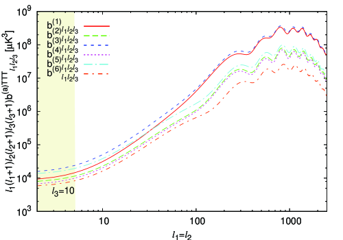
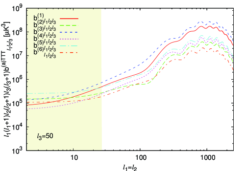
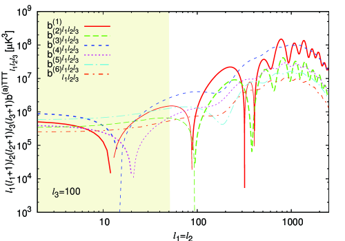
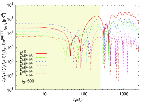
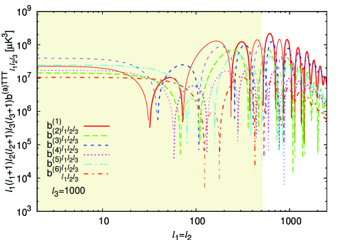
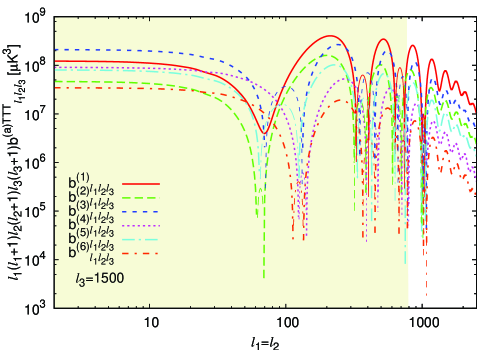
Figure 1: Shown are the temperature bispectra $b^{(a)TTT}_{l_{1}l_{2}l_{3}}$. $b^{(1)TTT}_{l_{1}l_{2}l_{3}}$ (solid red), $b^{(2)TTT}_{l_{1}l_{2}l_{3}}$ (short-dashed green), $b^{(3)TTT}_{l_{1}l_{2}l_{3}}$ (dotted blue), $b^{(4)TTT}_{l_{1}l_{2}l_{3}}$ (dot-dashed), $b^{(5)TTT}_{l_{1}l_{2}l_{3}}$ (long-dashed), $b^{(6)TTT}_{l_{1}l_{2}l_{3}}$ (dot-dot-dashed) in isosceles triangular configurations with $l_{1}=l_{2}$ are plotted as function of $l_{1}$ with fixed $l_{3}$. $l_{3}$ is set to 10 (top left), 50 (top middle), 100 (top right), 500 (bottom left), 1000 (bottom middle), 1500 (bottom right). In each panel, the shaded region at low multipoles shows configurations which fail to satisfy the triangular condition i.e. $|l_{1}-l_{2}|\geq l_{3}\geq l_{1}+l_{2}$.

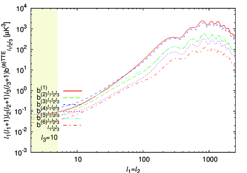
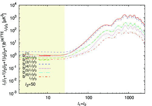
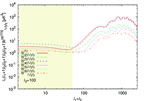
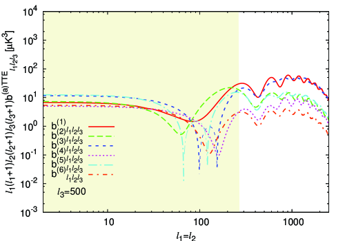
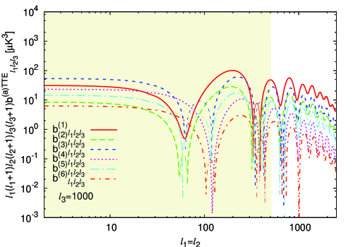
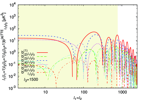
Figure 2: Same figure as in Fig. 1 but for $b^{(a)TTE}_{l_{1}l_{2}l_{3}}$.

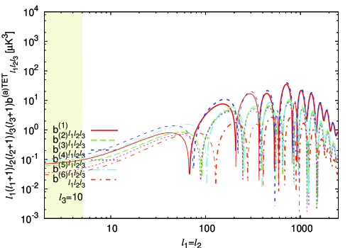
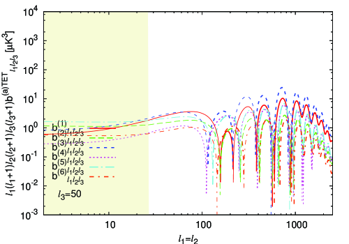
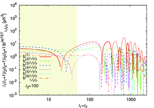
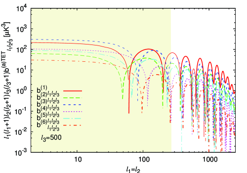
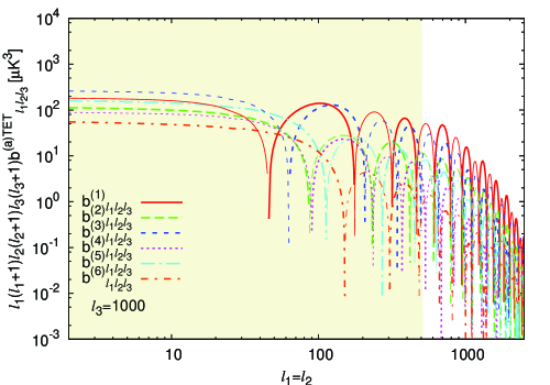
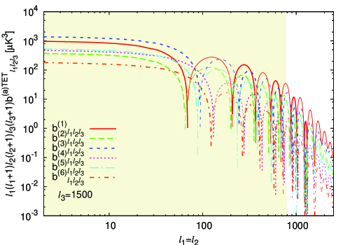
Figure 3: Same figure as in Fig. 1 but for $b^{(a)TET}_{l_{1}l_{2}l_{3}}$.

Fig. 1 shows the temperature bispectra $b^{(a)TTT}_{l_{1}l_{2}l_{3}}$ in isosceles triangular configurations with $l_{1}=l_{2}$. Cosmological parameters adopted here are the mean parameters for the flat power-law $\Lambda$CDM model from the WMAP 7-year result [2]. In numerical calculation, the transfer functions $g^{AP}_{l}(k)$ are computed using the CAMB code [43]. Among six bispectra $b^{(a)}_{l_{1}l_{2}l_{3}}$, $b^{(1)}_{l_{1}l_{2}l_{3}}$ and $b^{(3)}_{l_{1}l_{2}l_{3}}$ tend to be larger than others in most configurations, although configurations shown in the figure are limited. On the other hand, $b^{(6)}_{l_{1}l_{2}l_{3}}$ is in general the smallest. In addition, we can see there are peaks and troughs in the bispctra, which originate from the acoustic oscillation of the photon-baryon fluid prior to the recombination. As is discussed in Ref. [17], there is slight difference in the phase of the acoustic oscillation between the adiabatic and neutrino isocurvature density modes. This is due from the fact that while the acoustic oscillation in the adiabatic mode is dominantly sourced by the metric perturbations, that in the neutrino isocurvature density mode is dominated by the initial amplitudes (See Ref. [17] for more details). This makes the positions of acoustic peaks and troughs differ among bispectra. This can be prominently seen by comparing $b^{(1)}_{l_{1}l_{2}l_{3}}$ and $b^{(6)}_{l_{1}l_{2}l_{3}}$, which respectively originates purely from adiabatic and neutrino isocurvature density perturbations in Fig. 1. However, since the phase difference in acoustic oscillation is not as large as one between the adiabatic and matter isocurvature modes, the difference in positions of acoustic peaks is not prominent compared with the bispectra from mixture of adiabatic and matter isocurvature perturbations (See e.g. Ref. [29]).

We also plotted the bispectra arising from the correlation of two temperature and one polarization anisotropies, $b^{(a)TTE}_{l_{1}l_{2}l_{3}}$ and $b^{(a)TET}_{l_{1}l_{2}l_{3}}$ in Figs. 2 and 3, respectively. From these figures, we can see that above discussions on spectral shape of the bispectra are still qualitatively true when polarization is included.

4 Forecast for a CMB constraint

As we have seen, CMB bispectrum arising from the non-Gaussian isocurvature perturbations in extra radiation is distinct from the usual one from the non-Gaussian curvature perturbations. Therefore we can discriminate different non-Gaussinities in primordial perturbations from the observation of CMB anisotropy. To discuss this issue in a quantitative manner, we perform a Fisher matrix analysis.

In the limit of weak non-Gaussinity, the Fisher matrix for the non-Gaussianity parameters $f^{(a)}_{\rm NL}$ is given by [41, 42, 44]

$$F_{ab} = \sum_{l_{1}\leq l_{2}\leq l_{3}}\frac{(2l_{1}+1)(2l_{2}+1)(2l_{3}+1)}{4\pi}\begin{pmatrix}l_{1}&l_{2}&l_{3}\\ 0&0&0\end{pmatrix}^{2}$$ (37)

$$\times \sum_{P_{1}P_{2}P_{3}}\sum_{Q_{1}Q_{2}Q_{3}}b^{(a)~{}P_{1}P_{2}P_{3}}_{l_{1}l_{2}l_{3}}[\mathbf{Cov}^{-1}]^{P_{1}P_{2}P_{3}|Q_{1}Q_{2}Q_{3}}_{l_{1}l_{2}l_{3}}b^{(b)~{}Q_{1}Q_{2}Q_{3}}_{l_{1}l_{2}l_{3}},$$ (38)

where $[\mathbf{Cov}^{-1}]^{P_{1}P_{2}P_{3}|Q_{1}Q_{2}Q_{3}}_{l_{1}l_{2}l_{3}}$ is the inverse covariance matrix. Assuming that the observed sky coverage is unity and the instrumental noise is isotropic, the covariance matrix $[\mathbf{Cov}]^{P_{1}P_{2}P_{3}|Q_{1}Q_{2}Q_{3}}_{l_{1}l_{2}l_{3}}$ can be given as

$$[\mathbf{Cov}]^{P_{1}P_{2}P_{3}|Q_{1}Q_{2}Q_{3}}_{l_{1}l_{2}l_{3}}=\Delta_{l_{1}l_{2}l_{3}}\mathcal{C}^{P_{1}Q_{1}}_{l_{1}}\mathcal{C}^{P_{2}Q_{2}}_{l_{2}}\mathcal{C}^{P_{3}Q_{3}}_{l_{3}},$$ (39)

where $\mathcal{C}^{PQ}_{l}=C^{PQ}_{l}+N^{PQ}_{l}$ is the total angular power spectrum, which is the sum of ones from the CMB $C^{PQ}_{l}$ and instrumental noise $N^{PQ}_{l}$. $\Delta_{l_{1}l_{2}l_{3}}$ takes values 6, 2, 1 for the cases that all $l$’s are the same, only two of them are the same and otherwise, respectively.

Following [45], the noise power spectrum $N^{PQ}_{l}$ can be approximated as

$$N^{PQ}_{l}=\delta_{PQ}\theta_{\mathrm{FWHM}}^{2}\sigma_{P}^{2}\exp\left[l(l+1)\frac{\theta_{\mathrm{FWHM}}^{2}}{8\ln 2}\right],$$ (40)

where $\theta_{\mathrm{FWHM}}$ is the full width at half maximum of the Gaussian beam, and $\sigma_{P}$ is the root mean square of the instrumental noise par pixel. For cases of multi-frequency observations, $N^{PQ}_{l}$ is given via the quadrature sum over all the frequency bands. Here we study expected constraints from two survey. One is the on-going Planck survey [47] whose survey parameters are given in Table 1. Another is a hypothetical survey (hereafter CVL survey) whose sensitivity is limited by the cosmic variance, i.e. $N^{PQ}_{l}=0$. In both cases, we omit the effect of the sky cut and the sky coverage is assumed to be unity.

In the analysis, we consider only CMB bispectra from primordial non-Gaussianities, assuming contaminations from other sources are negligible. Since many of these sources including point sources and the thermal Sunyaev-Zel’dovich (SZ) effect have frequency spectra different from the black body, above assumption can be to some extent achieved by exploiting observations at multi-frequency bands. Other contaminations such as the lensing of CMB, the kinetic SZ effect, and the patchy reionization would not affect our results significantly.

As our models have six non-Gaussianity parameters $f^{(a)}_{\rm NL}$, the full Fisher matrix $F_{ab}$ is a $6\times 6$ matrix. However, it may sometimes occur that some of the parameters are not of primary interest and we want them to be marginalized over. In such the case, the Fisher matrix for the remaining non-Gaussianity parameters can be given as the inverse of the principal sub-matrix of the inverted full Fisher matrix [46].

bands [GHz]	$\theta_{\rm FWHM}$ [arcmin]	$\sigma_{T}$ [$\mu$K]	$\sigma_{P}$ [$\mu$K]
$30$	$33.0$	$2.0$	$2.8$
$44$	$24.0$	$2.7$	$3.9$
$70$	$14.0$	$4.7$	$6.7$
$100$	$10.0$	$2.5$	$4.0$
$143$	$7.1$	$2.2$	$4.2$
$217$	$5.0$	$4.8$	$9.8$
$353$	$5.0$	$14.7$	$29.8$

Table 1: Survey parameters adopted in our analysis for Planck. $\theta_{\rm FWHM}$ is Gaussian beam width at FWHM, $\sigma_{T}$ and $\sigma_{P}$ are temperature and polarization noise, respectively. We assume 1-year duration of observation.

In Figs. 4 and 5, shown are 2-dimensional constraints on the non-Gaussianity parameters expected for Planck and CVL surveys. Here we fixed $N_{\nu}$ to 4, which is suggested by recent observations we mentioned in Introduction. On each panel, constraints on a pair of $f^{(a)}_{\rm NL}$ are shown; other four non-Gaussianity parameters are marginalized over in Fig. 4 while they are fixed to zero in Fig. 5. Hereafter we will refer to constraints shown in Fig. 4 and 5 as marginalized and non-marginalized constraints, respectively.

Table 2: Expected uncertainties for non-Gaussianity parameters $\Delta f_{\rm NL}^{(a)}$ for the case with $N_{\rm eff}=4$.

survey	$f_{\rm NL}^{(1)}$	$f_{\rm NL}^{(2)}$	$f_{\rm NL}^{(3)}$	$f_{\rm NL}^{(4)}$	$f_{\rm NL}^{(5)}$	$f_{\rm NL}^{(6)}$
Planck	22	101	21	116	163	164
CVL	3.5	14.0	3.7	15.9	15.4	17.3

In Table 2, we listed expected uncertainties in the non-Gaussian parameters $\Delta f_{\rm NL}^{(a)}$, which are defined by

$$\Delta f_{\rm NL}^{(a)}\equiv F^{-1}_{aa}.$$ (41)

From the table as well as figures, we can see that among the six non-Gaussian parameters $f_{\rm NL}^{(a)}$, $f_{\rm NL}^{(1)}$ and $f_{\rm NL}^{(3)}$ can be constrained tighter than others. Planck (a CVL survey) can constrain $f_{\rm NL}^{(1)}$ and $f_{\rm NL}^{(3)}$ to about 20 (4). On the other hand, expected constraints on other $f_{\rm NL}^{(a)}$ are weaker with factor from five or eight. This result is consistent with our discussion in the previous section, where we showed that in the squeezed configurations, $b^{(1)P_{1}P_{2}P_{3}}_{l_{1}l_{2}l_{3}}$ and $b^{(3)P_{1}P_{2}P_{3}}_{l_{1}l_{2}l_{3}}$ are in general larger than other bispecra. We can also see that a CVL survey can significantly improve the constrains on all non-Gaussianity parameters from Planck by an order of magnitude. On the other hand, in the case of the matter isocurvature mode, constraints on some of non-Gaussianity parameters improve little as we measure higher and higher multipoles as shown in Ref. [35]. This difference reflects that CMB anisotropies at high multipoles are damped in the case of the matter isocurvature mode, while they are comparable in amplitude with the adiabatic mode in the extra radiation isocurvature mode.

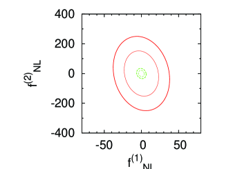
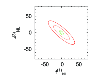
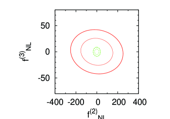
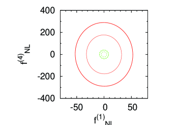
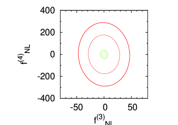
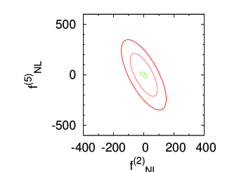
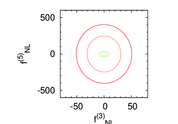
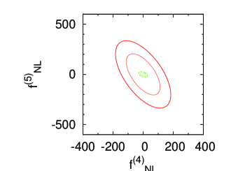
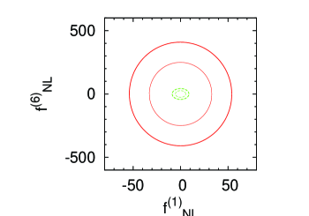
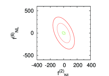
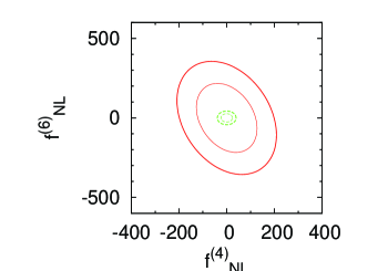
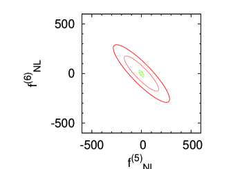
Figure 4: 2d marginalized constraints on the non-Gaussianity parameters $f^{(a)}_{\rm NL}$ expected for Planck (solid red) and CVL (dashed green) surveys. $N_{\nu}$ is fixed to $4$. Inner and outer contours correspond to constraints at 1 and 2 $\sigma$ levels.

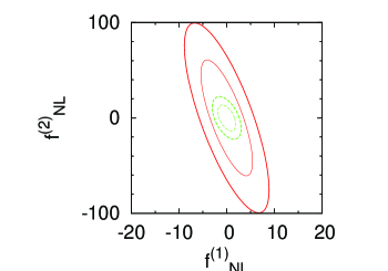
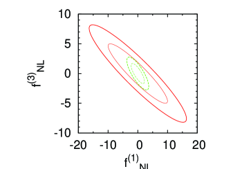
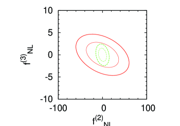
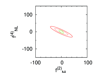
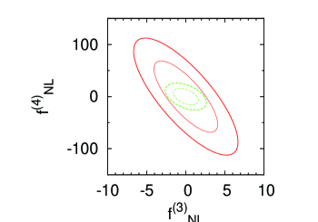
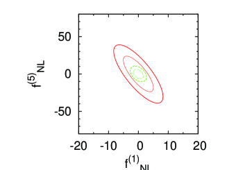
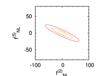
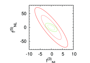
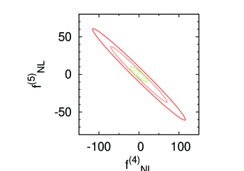
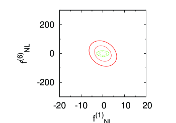
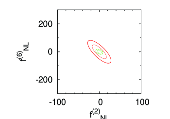
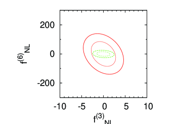
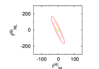
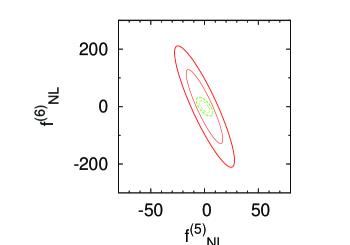
Figure 5: Same figure as in Fig. 4, but the non-marginalized constraints are shown here.

We also performed the same analysis for the case of fixed $N_{\nu}=3.04$. Marginalized and non-marginalized constraints on $f^{(a)}_{\rm NL}$ are shown in Figs. 6 and 7, respectively. Parameter uncertainties $\Delta f_{\rm NL}^{(a)}$ are listed in Table 3. In the context of isocurvature perturbations in extra radiation, such the case is realized when, while the fraction of extra radiation in energy density of DR is quite small, the amplitude of isocurvature perturbations in extra radiation $S_{\mathrm{X}}$ is large enough for the total DR isocurvature perturbations $S_{\mathrm{DR}}$ to be yet non-negligible. On the other hand, this is also naturally realized without extra radiation; $S_{\mathrm{DR}}$ is non-zero if there are isocurvature perturbations in the lepton number and non-Gaussian isocurvature perturbations in the lepton number may be produced in the Affleck-Dine mechanism, as shown in Sec. 5.2.

Compared with the case of $N_{\nu}=4$, constraints on $f^{(a)}_{\rm NL}$ are less stringent for the case of $N_{\nu}=3.04$. This can be understood as follows. As can be seen in Eqs. (3.23) and (3.24) of Ref. [17], given a fixed $S_{\rm DR}$, the initial perturbations is roughly proportional to the $\hat{R}_{\rm DR}\sim N_{\rm eff}$, where the $\hat{R}_{\rm DR}$ is the energy fraction of DR in the radiation component. Thus, apart from the effects of $N_{\rm eff}$ on the background evolution, the amplitude of CMB anisotropy from the dark radiation isocurvature perturbation should be proportional $N_{\rm eff}$, given a fixed $S_{\rm DR}$. Then the dependence of the bispectrum $b^{A_{1}P_{1},A_{2}P_{2}A_{3}P_{3}}_{l_{1}l_{2}l_{3}}$ on $N_{\rm eff}$ can be determined by the number of $A_{i}$ equals to $S_{\rm DR}$. Therefore we can expect $b^{(1)P_{1}P_{2}P_{3}}_{l_{1}l_{2}l_{3}}\propto{N_{\rm eff}}^{0}$, $b^{(2)P_{1}P_{2}P_{3}}_{l_{1}l_{2}l_{3}}\propto b^{(3)P_{1}P_{2}P_{3}}_{l_{1}l_{2}l_{3}}\propto N_{\rm eff}$ $b^{(4)P_{1}P_{2}P_{3}}_{l_{1}l_{2}l_{3}}\propto b^{(5)P_{1}P_{2}P_{3}}_{l_{1}l_{2}l_{3}}\propto{N_{\rm eff}}^{2}$ and $b^{(6)P_{1}P_{2}P_{3}}_{l_{1}l_{2}l_{3}}\propto{N_{\rm eff}}^{3}$. This can be converted into the dependence of $\Delta f_{\rm NL}$ on $N_{\rm eff}$. We can expect $\Delta f_{\rm NL}^{(1)}\propto{N_{\rm eff}}^{0}$, $\Delta f_{\rm NL}^{(2)}\propto\Delta f_{\rm NL}^{(3)}\propto{N_{\rm eff}}^{-1}$ $\Delta f_{\rm NL}^{(4)}\propto\Delta f_{\rm NL}^{(5)}\propto{N_{\rm eff}}^{-2}$ and $\Delta f_{\rm NL}^{(6)}\propto{N_{\rm eff}}^{-3}$. This rough estimate can be verified by comparing Tables 2 and 3.

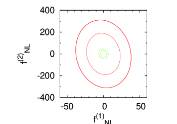
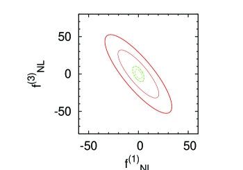
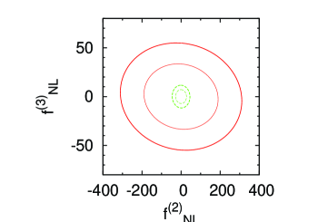
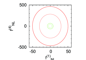
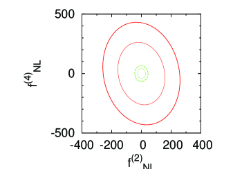
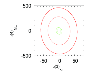
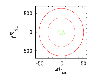
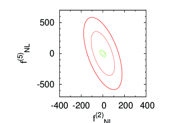
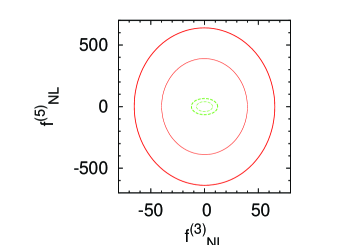
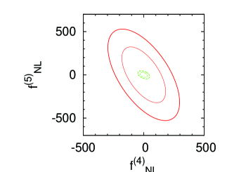
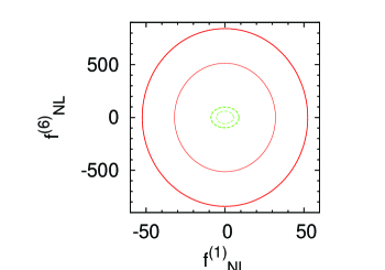
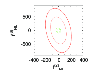
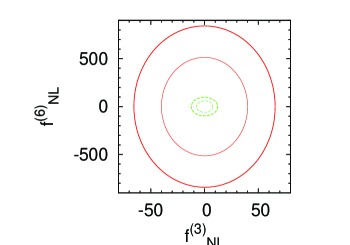
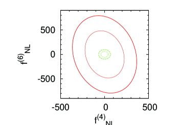
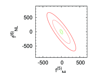
Figure 6: 2d marginalized constraints on non-Gaussianity parameters for $N_{\nu}=3.04$.

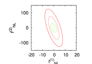
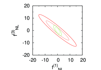
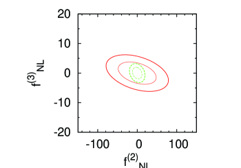
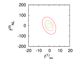
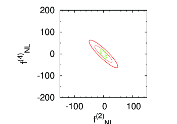
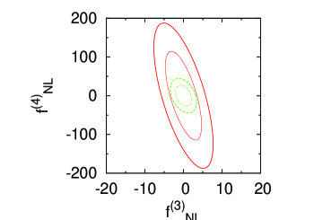
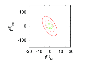
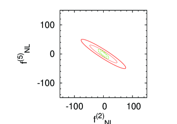
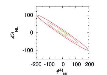
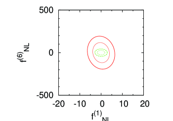
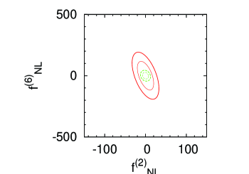
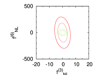
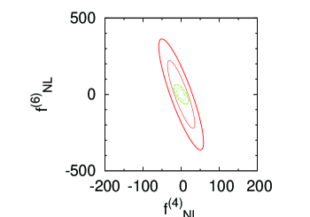
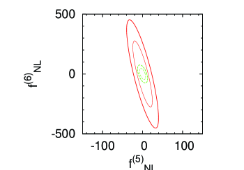
Figure 7: 2d non-marginalized constraints on non-Gaussianity parameters for $N_{\nu}=3.04$.

Table 3: Same as in Fig. 2, but for the case with $N_{\rm eff}=3.04$.

survey	$f_{\rm NL}^{(1)}$	$f_{\rm NL}^{(2)}$	$f_{\rm NL}^{(3)}$	$f_{\rm NL}^{(4)}$	$f_{\rm NL}^{(5)}$	$f_{\rm NL}^{(6)}$
Planck	21	126	27	187	257	339
CVL	3.5	18.3	5.0	27.2	26.4	39.3

5 Models for non-Gaussian isocurvature perturbations in dark radiation

In this section, we refer to some of particle physics models in which the DR isocurvature perturbations and their non-Gaussianities arise. We discuss two cases separately. In one scenario, the DR isocurvature perturbation is carried by extra light species. In the other scenario, ordinary neutrinos have large isocurvature perturbation.

5.1 Extra light species

Let us consider the cosmological scenario considered in Ref. [17] where two scalars, the inflaton $\phi$ and the curvaton $\sigma$, which is light during inflation, contribute to both the adiabatic and isocurvature perturbations. Using the $\delta N$ formalism [36, 37], the expansion coefficients of $\zeta$, such as $N_{\phi},~{}N_{\sigma}$, are given as

$$\begin{split}&N_{\phi}=\frac{1}{M_{\rm P}^{2}}\frac{V}{V_{\phi}},\\ &N_{\sigma}=\frac{3+R}{6\sigma_{i}}\left(\frac{\hat{R}_{r}R_{r}^{(\sigma)}}{R_{r}}+\frac{\hat{R}_{X}R_{X}^{(\sigma)}}{R_{X}}\right),\\ &N_{\phi\phi}=\frac{1}{M_{\rm P}^{2}}\left(1-\frac{VV_{\phi\phi}}{V_{\phi}^{2}}\right),\\ &N_{\sigma\sigma}=\frac{2}{9\sigma_{i}^{2}}\frac{3+R}{4}\left(\frac{\hat{R}_{r}R_{r}^{(\sigma)}}{R_{r}}+\frac{\hat{R}_{X}R_{X}^{(\sigma)}}{R_{X}}\right)\\ &~{}~{}~{}~{}~{}\times\left[3+4R-2R^{2}-2(3+R)\left(\frac{\hat{R}_{r}R_{r}^{(\sigma)}}{R_{r}}+\frac{\hat{R}_{X}R_{X}^{(\sigma)}}{R_{X}}\right)\right].\end{split}$$ (42)

In a similar manner, those of $S_{\rm DR}$ are given as

$$\begin{split}&S_{\sigma}=-\frac{3+R}{2\sigma_{i}}\frac{\hat{R}_{r}\hat{R}_{X}}{\hat{R}_{\rm DR}}\left(\frac{R_{r}^{(\sigma)}}{R_{r}}-\frac{R_{X}^{(\sigma)}}{R_{X}}\right)(1-\hat{c}_{\nu}),\\ &S_{\sigma\sigma}=\frac{3+R}{2\sigma_{i}^{2}}\frac{\hat{R}_{r}\hat{R}_{X}}{\hat{R}_{\rm DR}}\left(\frac{R_{r}^{(\sigma)}}{R_{r}}-\frac{R_{X}^{(\sigma)}}{R_{X}}\right)\frac{(1-\hat{c}_{\nu})}{3}\\ &~{}~{}~{}\times\left[2R^{2}-4R-3+\frac{3+R}{\hat{R}_{\rm DR}}\left(\frac{\hat{R}_{r}R_{r}^{(\sigma)}(\hat{c}_{\nu}+\hat{R}_{\rm DR})}{R_{r}}+\frac{\hat{R}_{X}R_{X}^{(\sigma)}(1+\hat{R}_{\rm DR})}{R_{X}}\right)\right],\\ &S_{\phi}=S_{\phi\phi}=0.\end{split}$$ (43)

The meanings of the symbols are as follows: $M_{P}$ is the reduced Planck mass. $V$ is the potential of $\phi$ and $V_{\phi}$ and $V_{\phi\phi}$ are the first and second derivatives of $V$, respectively, evaluated when observable scales exit the horizon. $R_{\sigma}$ is the ratio of the energy density of $\sigma$ to the total energy density at its decay and $R\equiv 3R_{\sigma}/(4-R_{\sigma})$. $R_{i}$ is the ratio of the energy density of a fluid $i$ to the total energy density at the decay of $\sigma$, and $\hat{R}_{i}$ is that at the electron-positron annihilation. The subscripts $r$, $X$ and DR mean the relativistic particles in the Standard Model, the extra radiation and the dark radiation, respectively. $R^{(\sigma)}_{i}$ is the ratio of energy density of the fluid $i$ generated by $\sigma$ decay at that time. $\sigma_{i}$ is the amplitude of the oscillation of $\sigma$ when it starts to oscillate. $\hat{c}_{\nu}\simeq 0.405$ is the ratio of the energy density of neutrino to that of standard model relativistic particles (photons and neutrinos) after the electron-positron annihilation. We can get (42) and (43) by comparing the energy densities of various components before and after the events such as $\sigma$ decay, neutrino decoupling and electron-positron annihilation, when the energy ratio of the standard model radiation and that of the dark radiation change, on the uniform density slice. Therefore (42) and (43) are written in terms of the energy ratio of each component at such events. The effective number of neutrino species in this scenario is

$$\Delta N_{\rm eff}=\frac{3\hat{R}_{X}}{\hat{c}_{\nu}\hat{R}_{r}}.$$ (44)

We refer to Ref. [17] for details and derivations of these quantities. Although these expression are rather lengthy, they are greatly simplified in some concrete situation, as will be seen in the following examples.

Using these quantities, the non-Gaussianity parameters defined in Eq. (9) are expressed as

$$f_{\rm NL}^{\zeta,\zeta\zeta}(k_{1},k_{2},k_{3}) \equiv \frac{N_{\phi}^{2}N_{\phi\phi}+N_{\sigma}^{2}N_{\sigma\sigma}}{(N_{\phi}^{2}+N_{\sigma}^{2})^{2}}+\frac{N_{\phi\phi}^{3}+N_{\sigma\sigma}^{3}}{(N_{\phi}^{2}+N_{\sigma}^{2})^{3}}\ln(k_{b}L)\Delta_{\zeta}^{2}(k_{1}),$$ (45)

$$f_{\rm NL}^{S_{\rm DR},\zeta\zeta}(k_{1},k_{2},k_{3}) \equiv \frac{N_{\sigma}^{2}S_{\sigma\sigma}}{(N_{\phi}^{2}+N_{\sigma}^{2})^{2}}+\frac{N_{\sigma\sigma}^{2}S_{\sigma\sigma}}{(N_{\phi}^{2}+N_{\sigma}^{2})^{3}}\ln(k_{b}L)\Delta_{\zeta}^{2}(k_{1}),$$

$$f_{\rm NL}^{\zeta,S_{\rm DR}\zeta}(k_{1},k_{2},k_{3}) = f^{\zeta,\zeta S_{\rm DR}}(k_{1},k_{2},k_{3})$$

$$\equiv \frac{N_{\sigma}S_{\sigma}N_{\sigma\sigma}}{(N_{\phi}^{2}+N_{\sigma}^{2})^{2}}+\frac{N_{\sigma\sigma}^{2}S_{\sigma\sigma}}{(N_{\phi}^{2}+N_{\sigma}^{2})^{3}}\ln(k_{b}L)\Delta_{\zeta}^{2}(k_{1}),$$

$$f_{\rm NL}^{\zeta,S_{\rm DR}S_{\rm DR}}(k_{1},k_{2},k_{3}) \equiv \frac{S_{\sigma}^{2}N_{\sigma\sigma}}{(N_{\phi}^{2}+N_{\sigma}^{2})^{2}}+\frac{N_{\sigma\sigma}S_{\sigma\sigma}^{2}}{(N_{\phi}^{2}+N_{\sigma}^{2})^{3}}\ln(k_{b}L)\Delta_{\zeta}^{2}(k_{1}),$$

$$f_{\rm NL}^{S_{\rm DR},\zeta S_{\rm DR}}(k_{1},k_{2},k_{3}) = f^{S_{\rm DR},S_{\rm DR}\zeta}(k_{1},k_{2},k_{3})$$

$$\equiv \frac{N_{\sigma}S_{\sigma}S_{\sigma\sigma}}{(N_{\phi}^{2}+N_{\sigma}^{2})^{2}}+\frac{N_{\sigma\sigma}S_{\sigma\sigma}^{2}}{(N_{\phi}^{2}+N_{\sigma}^{2})^{3}}\ln(k_{b}L)\Delta_{\zeta}^{2}(k_{1}),$$

$$f_{\rm NL}^{S_{\rm DR},S_{\rm DR}S_{\rm DR}}(k_{1},k_{2},k_{3}) \equiv \frac{S_{\sigma}^{2}S_{\sigma\sigma}}{(N_{\phi}^{2}+N_{\sigma}^{2})^{2}}+\frac{S_{\sigma\sigma}^{3}}{(N_{\phi}^{2}+N_{\sigma}^{2})^{3}}\ln(k_{b}L)\Delta_{\zeta}^{2}(k_{1}).$$ (48)

Here, we include the “quadratic” type components [40, 26, 29, 30, 32], which consist of three quadratic terms of $\delta\phi_{i}$ in each $\zeta$ or $S_{\rm DR}$, in addition to the leading “linear” components, which consist of a quadratic term in one of three $\zeta$ or $S_{\rm DR}$ and two linear terms from others. While $f_{\rm NL}^{\zeta,\zeta\zeta}$, etc. in Eqs. (45)-(48) are in principle not constant, their scale-dependences due from the factor $\ln(k_{b}L)\Delta_{\zeta}^{2}(k_{i})$ are quite moderate since $P_{\zeta}(k)$ is nearly scale-invariant. Therefore, so long as we consider observations sensitive to scales over only a few orders of magnitude, we can approximately ignore the scale-dependences. When we in the next section consider CMB signatures of non-Gaussian isocurvature perturbations in dark radiation, we adopt this approximation and regard the quantities $f_{\rm NL}^{\zeta,\zeta\zeta}$, etc. as constants. Then given constant $f_{\rm NL}^{\zeta,\zeta\zeta}$, etc., as shown in Eq. (7), the bispectra can be written as

$$B^{\zeta\zeta\zeta}(k_{1},k_{2},k_{3})=f_{\rm NL}^{\zeta,\zeta\zeta}\left[P_{\zeta}(k_{2})P_{\zeta}(k_{3})+\mbox{(2 cyclics of \{123\})}\right],$$ (49)

$$B^{\zeta\zeta S_{\rm DR}}(k_{1},k_{2},k_{3})=f_{\rm NL}^{\zeta,\zeta S_{\rm DR}}\left[P_{\zeta}(k_{2})P_{\zeta}(k_{3})+P_{\zeta}(k_{3})P_{\zeta}(k_{1})\right]+f_{\rm NL}^{S_{\rm DR},\zeta\zeta}P_{\zeta}(k_{1})P_{\zeta}(k_{2}),$$ (50)

$$B^{\zeta S_{\rm DR}S_{\rm DR}}(k_{1},k_{2},k_{3})=f_{\rm NL}^{\zeta,S_{\rm DR}S_{\rm DR}}P_{\zeta}(k_{2})P_{\zeta}(k_{3})$$ (51)

$$\hskip 142.26378pt+f_{\rm NL}^{S_{\rm DR},S_{\rm DR}\zeta}\left[P_{\zeta}(k_{3})P_{\zeta}(k_{1})+P_{\zeta}(k_{1})P_{\zeta}(k_{2})\right],$$

$$B^{S_{\rm DR}S_{\rm DR}S_{\rm DR}}(k_{1},k_{2},k_{3})=f_{\rm NL}^{S_{\rm DR},S_{\rm DR}S_{\rm DR}}\left[P_{\zeta}(k_{2})P_{\zeta}(k_{3})+\mbox{(2 cyclics of \{123\})}\right].$$ (52)

In the following subsections we consider two cases. One is the case where the $\sigma$ dominantly decays into extra light species $X$, while the curvature perturbation is dominantly generated by the inflaton (Sec. 5.1.1). The other is the case where the $\sigma$ decays into ordinary radiation and is the dominant source of the adiabatic perturbation, while extra light species are produced in thermal bath after the inflaton decay (Sec. 5.1.2). Both cases are realized in the framework of supersymmetric (SUSY) axion model [48] as mentioned in the previous work [17], and originally in Ref. [10]. We shall partly repeat discussions there.

5.1.1 Dark radiation from particle decay

Let us assume that the primordial curvature perturbation is dominantly produced by the inflaton : $N_{\phi}\gg N_{\sigma}$, and the inflaton decay only to the visible sector. This makes the isocurvature mode uncorrelated with the adiabatic mode. In this setup, we can approximate parameters as $R_{r}^{(\sigma)}\simeq 0$, and $R_{X}=R_{X}^{(\sigma)}\simeq R_{\sigma}\simeq 4R/3$. We also assume $R_{\sigma}<1$ since otherwise $\sigma$ dominates the Universe before it decays and the Universe would be dominated by $X$. Then Eqs. (42) and (43) are simplified as

$$\begin{split}&N_{\sigma}\simeq\frac{1}{2\sigma_{i}}\hat{R}_{X},\\ &N_{\sigma\sigma}\simeq\frac{1}{2\sigma_{i}^{2}}\hat{R}_{X},\\ &S_{\sigma}\simeq\frac{3}{2\sigma_{i}}\frac{1-\hat{c}_{\nu}}{\hat{c}_{\nu}}\hat{R}_{X}\simeq 3\frac{1-\hat{c}_{\nu}}{\hat{c}_{\nu}}N_{\sigma},\\ &S_{\sigma\sigma}\simeq\frac{3}{2\sigma_{i}^{2}}\frac{1-\hat{c}_{\nu}}{\hat{c}_{\nu}}\hat{R}_{X}\simeq 3\frac{1-\hat{c}_{\nu}}{\hat{c}_{\nu}}N_{\sigma\sigma}.\end{split}$$ (53)

Here and hereafter, we assume that the inflaton does not induce the non-Gaussianity, that is, $N_{\phi\phi}\simeq 0$. The quantity $\hat{R}_{X}$ is related to $R_{X}$ as [17]

$$\hat{R}_{X}\simeq\frac{1}{1+\delta}\left(\frac{g_{*}(H=\Gamma_{\nu})}{g_{*}(H=\Gamma_{\sigma})}\right)^{1/3}R_{X}.$$ (54)

Here $\delta=((11/4)^{1/3}-1)(1-c_{\nu})$, $c_{\nu}=\rho_{\nu}/\rho_{r}=21/43$ is the ratio of the energy of neutrinos to that of all visible matters at neutrino decoupling, $g_{*}(H=\Gamma_{\nu})$ is the relativistic degrees of freedom at that time and $g_{*}(H=\Gamma_{\sigma})$ is that at $\sigma$ decay. From Eq. (44), we can also express the effective number of neutrino species as

$$\Delta N_{\rm eff}\simeq\frac{4}{\hat{c}_{\nu}(1+\delta)}\left(\frac{g_{*}(H=\Gamma_{\nu})}{g_{*}(H=\Gamma_{\sigma})}\right)^{1/3}R.$$ (55)

Thus $\Delta N_{\rm eff}\sim 1$ if $R$ is not much smaller than one. Using (53), we get the relations among the non-Gaussianity parameters as

$$\begin{split}&f^{S_{\rm DR},\zeta\zeta}_{\rm NL}\simeq f^{\zeta,S_{\rm DR}\zeta}_{\rm NL}\simeq 3\frac{1-\hat{c}_{\nu}}{\hat{c}_{\nu}}f^{\zeta,\zeta\zeta}_{\rm NL},\\ &f^{\zeta,S_{\rm DR}S_{\rm DR}}_{\rm NL}\simeq f^{S_{\rm DR},\zeta S_{\rm DR}}_{\rm NL}\simeq 9\left(\frac{1-\hat{c}_{\nu}}{\hat{c}_{\nu}}\right)^{2}f^{\zeta,\zeta\zeta}_{\rm NL},\\ &f^{S_{\rm DR},S_{\rm DR}S_{\rm DR}}_{\rm NL}\simeq 27\left(\frac{1-\hat{c}_{\nu}}{\hat{c}_{\nu}}\right)^{3}f^{\zeta,\zeta\zeta}_{\rm NL}.\end{split}$$ (56)

Thus these non-Gaussianity parameters are comparable. The magnitude of them is roughly given by

$$f^{\zeta,\zeta\zeta}_{\rm NL}(k_{1},k_{2},k_{3}) \simeq\frac{N_{\sigma}^{2}N_{\sigma\sigma}}{N_{\phi}^{4}}+\frac{N_{\sigma\sigma}^{3}}{N_{\phi}^{6}}\ln(k_{b}L)\Delta_{\zeta}^{2}(k_{1})$$

$$\sim\epsilon^{2}\left(\frac{M_{\rm P}}{\sigma_{i}}\right)^{4}\hat{R}_{X}^{3}+\epsilon^{3}\left(\frac{M_{\rm P}}{\sigma_{i}}\right)^{6}\hat{R}_{X}^{3}\Delta_{\zeta}^{2}(k_{1}),$$ (57)

where $\epsilon=\frac{1}{2}M_{\rm P}^{2}(V_{\phi}/V)^{2}$ is the slow-roll parameter. It is easily found that the first term is of the order of $(P_{S_{\rm DR}}/P_{\zeta})^{2}\times(1/\hat{R}_{X})$ while the second term is of the order of $(P_{S_{\rm DR}}/P_{\zeta})^{3}\times(\Delta_{\zeta}^{2}/\hat{R}_{X}^{3})$. Therefore, the non-linearity parameter can be large enough to be probed for not so small $P_{S_{\rm DR}}$ compared to $P_{\zeta}$ and $\hat{R}_{X}\ll 1$. Thus even if $R_{X}$ is very small and there is no significant deviation from $N_{\rm eff}=3.046$, the DR isocurvature mode and its non-Gaussianity may be detected.

Now let us estimate $\hat{R}_{X}\sim R$ and $S_{\rm DR}$ in the SUSY KSVZ axion model [50]. In a SUSY axion model [49], the saxion $\sigma$, the scalar partner of the PQ axion, exists and has a mass $m_{\sigma}$ which ranges from $\mathcal{O}({\rm keV})$ to $\mathcal{O}({\rm TeV})$, in accordance with the SUSY breaking scale. The saxion can have a large initial amplitude $\sigma_{i}$ during inflation, and may obtain quantum fluctuations $\delta\sigma\sim H_{\rm inf}/2\pi$ if it is much lighter than the Hubble parameter during inflation. In this model, the dominant decay channel of the saxion is typically that into two axions. Relativistic axions produced by the saxion decay behave as an extra radiation $X$, since they are decoupled from ordinary matter almost completely. Here the $R\simeq 3R_{\sigma}/4$ is given by [17]

$$R\simeq 2\times 10^{-4}\left(\frac{T_{\rm R}}{10^{6}{\rm GeV}}\right)\left(\frac{1{\rm GeV}}{m_{\sigma}}\right)^{3/2}\left(\frac{f_{a}}{10^{12}{\rm GeV}}\right)^{3}\left(\frac{\sigma_{i}}{f_{a}}\right)^{2},$$ (58)

for $R\ll 1$ and $m_{\sigma}>\Gamma_{\phi}$ and

$$R\simeq 2\times 10^{-3}\left(\frac{1{\rm GeV}}{m_{\sigma}}\right)\left(\frac{f_{a}}{10^{12}{\rm GeV}}\right)^{3}\left(\frac{\sigma_{i}}{f_{a}}\right)^{2},$$ (59)

for $R\ll 1$ and $m_{\sigma}<\Gamma_{\phi}$, where $f_{a}$ is the PQ symmetry breaking scale, $T_{\rm R}$ is the reheating temperature after the inflation and $\Gamma_{\phi}$ is the decay rate of the inflaton. Correspondingly, the magnitude of the DR isocurvature perturbation is given by

$$S_{\rm DR}\simeq 4\times 10^{-7}\left(\frac{T_{\rm R}}{10^{6}{\rm GeV}}\right)\left(\frac{1{\rm GeV}}{m_{\sigma}}\right)^{3/2}\left(\frac{f_{a}}{10^{12}{\rm GeV}}\right)^{2}\left(\frac{H_{\rm inf}}{10^{10}{\rm GeV}}\right)\left(\frac{\sigma_{i}}{f_{a}}\right),$$ (60)

for $R\ll 1$ and $m_{\sigma}>\Gamma_{\phi}$ and

$$S_{\rm DR}\simeq 4\times 10^{-6}\left(\frac{1{\rm GeV}}{m_{\sigma}}\right)\left(\frac{f_{a}}{10^{12}{\rm GeV}}\right)^{2}\left(\frac{H_{\rm inf}}{10^{10}{\rm GeV}}\right)\left(\frac{\sigma_{i}}{f_{a}}\right),$$ (61)

for $R\ll 1$ and $m_{\sigma}<\Gamma_{\phi}$. Here $S_{\rm DR}$ is regarded as $S_{\rm DR}=\sqrt{(k^{3}/2\pi^{2})P_{S_{\rm DR}S_{\rm DR}}}$ which should be compared with $\sqrt{(k^{3}/2\pi^{2})P_{\zeta\zeta}}\simeq 5\times 10^{-5}$. Thus the magnitude of the DR isocurvature perturbation can be sizable.

5.1.2 Dark radiation from thermal bath

Next, we consider the case $\sigma$ takes a role of the curvaton, and hence it dominantly sources the adiabatic perturbation : $N_{\sigma}\gg N_{\phi}$. Moreover, we assume that the inflaton decays into ordinary radiation with a branching ratio $r_{\phi}$, and into $X$ with a branching ratio $1-r_{\phi}$. The curvaton $\sigma$ is assumed to decay only into ordinary radiation. In this model, we make use of following approximations : $R^{(\sigma)}_{r}\simeq R_{\sigma}(\sim 4R/3)$, $R^{(\sigma)}_{X}\simeq 0$. We also assume $R_{\sigma}<1$ since otherwise the $\sigma$ decay releases huge amount of entropy and it dilutes the $X$ abundance significantly. Under these assumptions, Eqs. (42) and (43) are simplified as

$$\begin{split}&N_{\sigma}\simeq\frac{2R}{3\sigma_{i}},\\ &N_{\sigma\sigma}\simeq\frac{2R}{3\sigma_{i}^{2}},\\ &S_{\sigma}\simeq-3\frac{1-\hat{c}_{\nu}}{\hat{c}_{\nu}}\hat{R}_{X}\frac{2R}{3\sigma_{i}}\simeq-3\frac{1-\hat{c}_{\nu}}{\hat{c}_{\nu}}\hat{R}_{X}N_{\sigma},\\ &S_{\sigma\sigma}\simeq-3\frac{1-\hat{c}_{\nu}}{\hat{c}_{\nu}}\hat{R}_{X}\frac{2R}{3\sigma_{i}^{2}}\simeq-3\frac{1-\hat{c}_{\nu}}{\hat{c}_{\nu}}\hat{R}_{X}N_{\sigma\sigma}.\end{split}$$ (62)

The relation between $\hat{R}_{X}$ and $R_{X}$ is given by Eq. (54) where $R_{X}$ is given by

$$R_{X}=(1-r_{\phi})(1-R_{\sigma}).$$ (63)

In this model, $\Delta N_{\rm eff}$ is given by

$$\Delta N_{\rm eff}\simeq\frac{3}{\hat{c}_{\nu}(1+\delta)}\left(\frac{g_{*}(H=\Gamma_{\nu})}{g_{*}(H=\Gamma_{\sigma})}\right)^{1/3}(1-r_{\phi}).$$ (64)

The relationships among the non-Gaussianity parameters become

$$\begin{split}&f^{S_{\rm DR},\zeta\zeta}_{\rm NL}\simeq f^{\zeta,S_{\rm DR}\zeta}_{\rm NL}\simeq-3\frac{1-\hat{c}_{\nu}}{\hat{c}_{\nu}}\hat{R}_{X}f^{\zeta,\zeta\zeta}_{\rm NL},\\ &f^{\zeta,S_{\rm DR}S_{\rm DR}}_{\rm NL}\simeq f^{S_{\rm DR},\zeta S_{\rm DR}}_{\rm NL}\simeq 9\left(\frac{1-\hat{c}_{\nu}}{\hat{c}_{\nu}}\right)^{2}\hat{R}_{X}^{2}f^{\zeta,\zeta\zeta}_{\rm NL},\\ &f^{S_{\rm DR},S_{\rm DR}S_{\rm DR}}_{\rm NL}\simeq-27\left(\frac{1-\hat{c}_{\nu}}{\hat{c}_{\nu}}\right)^{3}\hat{R}_{X}^{3}f^{\zeta,\zeta\zeta}_{\rm NL}.\end{split}$$ (65)

In this case,

$$f^{S_{\rm DR},S_{\rm DR}S_{\rm DR}}_{\rm NL}\ll f^{\zeta,S_{\rm DR}S_{\rm DR}}_{\rm NL}\simeq f^{S_{\rm DR},\zeta S_{\rm DR}}_{\rm NL}\ll f^{S_{\rm DR},\zeta\zeta}\simeq f^{\zeta,S_{\rm DR}\zeta}_{\rm NL}\ll f^{\zeta,\zeta\zeta}.$$ (66)

This is because $\sigma$, which is the origin of the non-Gaussianity, dominantly decays to visible particles. Since we assume that the primordial curvature perturbation is dominantly produced by $\sigma$. the non-linearity parameter for the adiabatic perturbation is given by

$$f_{\rm NL}^{\zeta,\zeta\zeta}(k_{1},k_{2},k_{3})\simeq\frac{3}{2R}+\frac{27}{8R^{3}}\ln(k_{b}L)\Delta^{2}_{\zeta}(k_{1}).$$ (67)

We see that the non-Gaussianity in the adiabatic perturbation becomes large for $R\ll 1$ while that of the DR isocurvature mode is given by $f_{\rm NL}^{S_{\rm DR},\zeta\zeta}\sim f_{\rm NL}^{\zeta,S_{\rm DR}\zeta}\sim(P_{\rm S_{\rm DR}}/P_{\zeta})^{1/2}\times(1/R)$, can be order unity if $P_{S_{\rm DR}}$ is close to the observational upper bound, or $\hat{R}_{X}$ is close to unity.

The above situation is actually realized in the SUSY DFSZ axion model [51] once the saxion is identified as the curvaton $\sigma$ and the axion as the extra light species $X$. In this model, the dominant decay channel of the saxion may be that into a Higgs boson pair. Therefore, the energy of saxion is almost converted to visible particles. On the other hand, there may be axions produced from the thermal bath during reheating. Let us suppose that the reheating temperature is high so that it satisfies $T_{\rm R}\gtrsim T_{\rm D}$, where $T_{\rm D}\simeq 10^{7}{\rm GeV}(f_{a}/10^{10}{\rm GeV})^{2.246}$ is the temperature at the axion decoupling from thermal bath [52]. Thus axions are thermalized after the inflaton decay. The ratio of the axion energy density to the total energy density at the axion decoupling is given by $g_{*}(T=T_{\rm D})^{-1}$. The inflaton decay branching ratio into $X$, $1-r_{\phi}$, is replaced by the ratio of the energy density of axions to that of the whole radiation originating from the inflaton at the epoch of saxion decay. Thus it is estimated to be

$$1-r_{\phi}=\frac{1}{g_{*}(T=T_{\rm D})}\left(\frac{g_{*}(H=\Gamma_{\sigma})}{g_{*}(T=T_{\rm D})}\right)^{1/3},$$ (68)

where $\Gamma_{\sigma}$ is the saxion decay rate. From this, we see that $1-r_{\phi}$ is typically much smaller than $1$. Eventually, the amount of axions is smaller than that of visible particles whether they are produced by the inflaton or the saxion. Then we have $R_{X}\ll 1$ from Eq. (63). The ratio of the saxion energy density to the total energy density at the epoch of saxion decay is given by

$$R\simeq 7\times 10^{-2}\left(\frac{T_{\rm R}}{10^{6}{\rm GeV}}\right)\left(\frac{m_{\sigma}}{1{\rm GeV}}\right)^{1/2}\left(\frac{1{\rm TeV}}{\mu}\right)^{2}\left(\frac{f_{a}}{10^{15}{\rm GeV}}\right)^{3}\left(\frac{\sigma_{i}}{f_{a}}\right)^{2},$$ (69)

for $m_{\sigma}>\Gamma_{\phi}$ and

$$R\simeq 7\times 10^{-1}\left(\frac{m_{\sigma}}{1{\rm GeV}}\right)\left(\frac{1{\rm TeV}}{\mu}\right)^{2}\left(\frac{f_{a}}{10^{15}{\rm GeV}}\right)^{3}\left(\frac{\sigma_{i}}{f_{a}}\right)^{2},$$ (70)

for $m_{\sigma}<\Gamma_{\phi}$, where $\mu$ denotes the higgsino mass. The magnitude of the DR isocurvature perturbation is given by

$$S_{\rm DR}\simeq 6\times 10^{-7}\left(\frac{T_{\rm R}}{10^{6}{\rm GeV}}\right)\left(\frac{m_{\sigma}}{1{\rm GeV}}\right)^{1/2}\left(\frac{1{\rm TeV}}{\mu}\right)^{2}\left(\frac{f_{a}}{10^{15}{\rm GeV}}\right)^{2}\left(\frac{H_{\rm inf}}{10^{13}{\rm GeV}}\right)\left(\frac{\sigma_{i}}{f_{a}}\right),$$ (71)

for $m_{\sigma}>\Gamma_{\phi}$ and

$$S_{\rm DR}\simeq 6\times 10^{-6}\left(\frac{m_{\sigma}}{1{\rm GeV}}\right)\left(\frac{1{\rm TeV}}{\mu}\right)^{2}\left(\frac{f_{a}}{10^{15}{\rm GeV}}\right)^{2}\left(\frac{H_{\rm inf}}{10^{13}{\rm GeV}}\right)\left(\frac{\sigma_{i}}{f_{a}}\right),$$ (72)

for $m_{\sigma}<\Gamma_{\phi}$, where we have used $g_{*}(T=T_{\rm D})=228.75$. Thus the DR isocurvature perturbation can be sizable for some parameter choices even if $R_{X}$ is much smaller then unity.

5.2 Large lepton asymmetry

Next, let us consider the case where the neutrino number density has an isocurvature perturbation. First note that neutrinos are in thermal equilibrium before the decoupling at $T\sim 1$ MeV. Thus neutrinos can only have an adiabatic perturbation unless they are produced after the decoupling or they have a chemical potential, i.e., there is asymmetry in the neutrino sector. We consider the latter possibility hereafter. The lepton number is conserved well after the electroweak symmetry breaking (EWSB) since the sphaleron effect [53] is suppressed. Therefore, if the asymmetry in the lepton number, $n_{L}-n_{\bar{L}}$, is created after the EWSB, it survives thereafter. Thus spatial fluctuations in the lepton asymmetry on large scales, if exist, are also conserved. This opens up a possibility that an observable (non-Gaussian) isocurvature perturbation in the lepton asymmetry, or the neutrino density isocurvature perturbation, is created after the EWSB [54]. The asymmetric part, $|n_{\nu}-n_{\bar{\nu}}|$, adds to the ordinary neutrino number density and hence it may significantly contribute to the $N_{\rm eff}$ as well as $S_{\rm DR}$ if the lepton asymmetry and its isocurvature perturbation are large enough. A concrete example was given in Ref. [55], where it was shown that the late decay of Q-balls can create large lepton asymmetry. It is interesting because we do not need an extra radiation particle $X$ to produce significant amount of DR isocurvature perturbation. Let us follow the arguments of Ref. [55] and estimate $\Delta N_{\rm eff}$ and $S_{\rm DR}$ in this model.

A large lepton asymmetry is created through the Affleck-Dine (AD) mechanism [56, 57]. Specifically, we make use of the $LL\bar{e}$ flat direction (also called as the AD field) [57, 58]. It does not have the baryon number, and hence it can create large lepton asymmetry without producing too much baryon asymmetry. If the AD field fragments into Q-balls [59] in which almost all the lepton number is confined [60, 61, 62, 63] and they evaporate after the EWSB, a large lepton asymmetry is released and it does not washed out. Since the AD field may obtain quantum fluctuations in its angular component during inflation [64, 65], it results in the isocurvature fluctuation in the lepton asymmetry, i.e., the neutrino density (non-Gaussian) isocurvature perturbation. Non-Gaussianity in the baryonic isocurvature perturbation generated through the AD mechanism was studied in Ref. [27].

We denote by $\psi$ the AD field along the $LL\bar{e}$ flat direction. It is lifted by the dimension six operator in the superpotential, $W=\psi^{6}/(6M^{3})$ with $M$ being the cutoff scale. We assume the gauge-mediated SUSY breaking model [66] in the following. The scalar potential for the AD field is given by [67]

$$V=(m_{3/2}^{2}-cH^{2})|\psi|^{2}+M_{F}^{4}\left(\log\frac{|\psi|^{2}}{M_{\rm mess}^{2}}\right)^{2}+\left(a_{m}m_{3/2}\frac{\psi^{6}}{6M^{3}}+{\rm h.c.}\right)+\frac{|\psi|^{10}}{M^{6}},$$ (73)

for $|\psi|>M_{\rm mess}$, where $M_{\rm mess}$ is the messenger scale, $m_{3/2}$ denotes the gravitino mass, $a_{m}$ is a constant of order unity and $M_{F}^{4}\simeq m_{\rm soft}^{2}M_{\rm mess}^{2}$ with $m_{\rm soft}\sim 1$ TeV.

The lepton number generated through the AD mechanism is estimated as

$$\begin{split}\frac{n_{L}}{s}&\simeq\frac{T_{\rm R}|\psi_{\rm os}|^{2}}{4m_{3/2}M_{P}^{2}}\sin(6\theta)\\ &\sim 5\times 10^{-3}\left(\frac{T_{\rm R}}{10^{5}\,{\rm GeV}}\right)\left(\frac{1\,{\rm GeV}}{m_{3/2}}\right)^{1/2}\left(\frac{M}{10^{20}\,{\rm GeV}}\right)^{3/2}\sin(6\theta),\end{split}$$ (74)

where $T_{\rm R}$ is the reheating temperature, $\theta$ is the initial angle of the AD field in the complex plane, and $|\psi_{\rm os}|\sim(m_{3/2}M^{3})^{1/4}$ is the AD field amplitude at the onset of its oscillation. It can be checked that thermal effects on the AD field potential is neglected in this parameter choice [68, 69]. The AD field fragments into Q-balls after it starts to oscillate, and they once dominate the Universe before they decay if $T_{d}<(T_{\rm R}/3)(|\psi_{\rm os}|/M_{P})^{2}$, where $T_{d}$ is the decay temperature of the Q-ball discussed later. In this case, the expression becomes $n_{L}/s\simeq(T_{d}/4m_{3/2})\sin(6\theta)$. Hereafter we regard the lepton asymmetry, denoted by the subscript $L$, as if it is an extra radiation component, which has been denoted by $X$ in the previous sections. The neutrino asymmetry in each flavor is expressed in terms of the chemical potential (or the degeneracy parameter) $\xi_{\nu_{i}}$ as

$$\frac{n_{L}}{n_{\gamma}}=\sum_{i=e,\mu,\tau}\frac{n_{\nu_{i}}-n_{\bar{\nu}_{i}}}{n_{\gamma}}=\sum_{i=e,\mu,\tau}\frac{1}{12\zeta(3)}\left(\frac{T_{\nu_{i}}}{T_{\gamma}}\right)^{3}(\pi^{2}\xi_{\nu_{i}}+\xi_{\nu_{i}}^{3}).$$ (75)

The neutrino chemical potentials contribute to the extra radiation energy density through the relation

$$\Delta N_{\rm eff}=\frac{3\rho_{L}}{\rho_{\nu}}=\sum_{i=e,\mu,\tau}\left[\frac{30}{7}\left(\frac{\xi_{\nu_{i}}}{\pi}\right)^{2}+\frac{15}{7}\left(\frac{\xi_{\nu_{i}}}{\pi}\right)^{4}\right].$$ (76)

Note however that the chemical potential of the electron neutrino directly affects the helium abundance [70] and hence its contribution to the radiation energy density is constrained as $\Delta N_{\rm eff}\lesssim\mathcal{O}(0.1)$ depending on the neutrino mixing angle $\theta_{13}$ [71]. Thus hereafter we neglect the contribution of the lepton asymmetry to the DR energy density, although the effect of its isocurvature perturbation may not be neglected.

The angular component of the AD field may be light during inflation [65] and it leads to the isocurvature perturbation in the lepton asymmetry. The isocurvature perturbation of the lepton asymmetry is calculated as

$$S_{L}=n\cot(n\theta)\delta\theta-\frac{1}{2}n^{2}(\delta\theta)^{2},$$ (77)

where $\sqrt{\langle\delta\theta^{2}\rangle}=H_{\rm inf}/(2\pi|\psi_{i}|)$, with $H_{\rm inf}$ being the Hubble scale during inflation and $n=6$ in the present model. The DR isocurvature perturbation is then estimated as

$$\begin{split}S_{\rm DR}&=\frac{\rho_{L}}{\rho_{\rm DR}}\left(S_{L}+\frac{2}{3}\frac{\rho_{\nu}}{\rho_{\rm DR}}S_{L}^{2}\right)\simeq\frac{\rho_{L}}{\rho_{\nu}}\left(S_{L}+\frac{2}{3}S_{L}^{2}\right)\\ &\sim 6\times 10^{-8}\left(\frac{T_{\rm R}}{10^{5}\,{\rm GeV}}\right)^{2}\left(\frac{m_{3/2}}{1\,{\rm GeV}}\right)^{-1}\left(\frac{M}{10^{20}\,{\rm GeV}}\right)^{9/4}\left(\frac{H_{\rm inf}}{10^{14}\,{\rm GeV}}\right)^{3/4},\end{split}$$ (78)

where $\rho_{\rm DR}=\rho_{L}+\rho_{\nu}$ denotes the DR energy density. In the second equality, we have neglected the contribution of the lepton asymmetry to the DR energy density for the reason discussed above. In the last equality, we have considered only the leading term. In the case of Q-ball domination, we obtain

$$S_{\rm DR}\sim 2\times 10^{-8}\left(\frac{T_{d}}{10\,{\rm MeV}}\right)^{2}\left(\frac{1\,{\rm GeV}}{m_{3/2}}\right)^{2}\left(\frac{M}{10^{20}\,{\rm GeV}}\right)^{-3/4}\left(\frac{H_{\rm inf}}{10^{14}\,{\rm GeV}}\right)^{3/4}.$$ (79)

Expanding the DR isocurvature perturbation as $S_{\rm DR}\simeq S_{\theta}\delta\theta+(1/2)S_{\theta\theta}(\delta\theta)^{2}$, we obtain

$$\begin{split}S_{\theta}&=\frac{\Delta N_{\rm eff}}{3}n\cot(n\theta),\\ S_{\theta\theta}&=-\frac{\Delta N_{\rm eff}}{3}n^{2}\left[1-\frac{4}{3}\cot^{2}(n\theta)\right].\end{split}$$ (80)

Therefore, we obtain the non-linearity parameter for the DR isocurvature perturbation as

$$f_{\rm NL}^{S_{\rm DR},S_{\rm DR}S_{\rm DR}}=\frac{S_{\theta}^{2}S_{\theta\theta}}{N_{\phi}^{4}|\psi_{i}|^{4}}+\frac{S_{\theta\theta}^{3}}{N_{\phi}^{6}|\psi_{i}|^{6}}\ln(k_{b}L)\Delta_{\zeta}^{2}(k_{1}).$$ (81)

It is easily checked that the first term is of the order of $(P_{S_{\rm DR}}/P_{\zeta})^{2}\times(\tan^{2}(n\theta)/\Delta N_{\rm eff})$. Thus the non-linearity parameter can be large enough to be probed for not so small $P_{S_{\rm DR}}$ compared to $P_{\zeta}$ and $\Delta N_{\rm eff}\ll 1$ or $\tan^{2}(n\theta)\gg 1$.

Finally we comment on the Q-ball formation in the present model, which is essential for protecting the lepton number from the sphaleron process. After the AD field starts to oscillate, the instability develops and Q-balls are formed. We consider the “delayed”-type Q-balls [62], which are formed when the AD field potential becomes dominated by the logarithmic term in (73). Then the charge of Q-ball is estimated as [62]

$$Q\sim\beta\left(\frac{M_{F}}{m_{3/2}}\right)^{4}\sim 6\times 10^{20}\left(\frac{1\,{\rm GeV}}{m_{3/2}}\right)^{4}\left(\frac{M_{F}}{10^{6}\,{\rm GeV}}\right)^{4},$$ (82)

where $\beta=6\times 10^{-4}$, and the radius of the Q-ball is given by $R_{Q}\sim m_{3/2}^{-1}$. Although almost all the lepton number created by the AD mechanism is absorbed into Q-balls, they can decay into neutrinos from their surfaces. The decay rate is given by $\Gamma_{Q}\sim Am_{3/2}^{3}/(192\pi^{3}Q)$ where $A$ is a surface area of the Q-ball [72]. Then the Q-ball decay temperature, $T_{d}$, is calculated as

$$T_{d}\simeq 3\times 10^{-2}\,{\rm GeV}\left(\frac{m_{3/2}}{1\,{\rm GeV}}\right)^{5/2}\left(\frac{10^{6}\,{\rm GeV}}{M_{F}}\right)^{2}.$$ (83)

This is well below the electroweak scale. Thus the lepton number liberated by the Q-ball decay is not converted into the baryon number. Notice that the Q-ball decay rate and hence its decay temperature depends on the charge $Q$. Thus if the $Q$ depends on the initial angle of the AD field $\theta$, the decay rate fluctuates on large scales and it causes the modulated reheating [75] for the case of Q-ball domination. In this case, the magnitude of the DR isocurvature perturbation is modified up to an $\mathcal{O}(1)$ numerical factor. In the GMSB, however, it is often the case that the ellipticity of the AD field orbit in the complex plane is small and the $Q$ does not depend on $\theta$ [62]. Therefore, there is no such an effect.

6 Summary

In this paper, we discussed non-Gaussianities in dark radiation isocurvature perturbations. Extending our analysis in the previous work [17], we first derived the primordial bispectrum originating from the non-Gaussian isocurvature perturbations in dark radiation. We presented primordial bispectra of both the local and quadratic types. As far as primordial perturbations have nearly scale-invariant spectra, amplitude of primordial power spectra can be parameterized with six non-Gaussian parameters, which consequently measure the non-Gaussianities in the mixture of the adiabatic and dark radiation isocurvature modes. We also presented CMB bispectrum from these non-Gaussianities, which allows us to forecast constraints on the non-Gaussian parameters from future CMB surveys including the Planck sattelite and a hypothetical CVL survey. While these parameters can be more or less constrained from ongoing Planck satellite experiments, there can be still some room for future CMB surveys to improve the constraint, and CMBpol [76] and COrE [77] missions are desirable to improve the constraints. We referred to SUSY axion models as concrete models for non-Gaussian dark radiation isocurvature perturbations and showed that they offer distinct signatures on amplitudes in the primordial bispectrum. We have also shown that non-vanishing $S_{\rm DR}$, imprinted in the lepton asymmetry, or the neutrino density isocurvature perturbation, can be generated through the Affleck-Dine mechanism without producing sizable extra radiation energy density. Since observational signatures are the same as those in the isocurvature model of the extra radiation component, primordial non-Gaussianities in the neutrino density isocurvature perturbation can also be constrained by CMB observations.

Extra radiation with $\Delta N_{\rm eff}\simeq 1$ will be tested by the ongoing Planck survey with high significance and its origin may be identified through the detection of extra radiation isocurvature perturbations. Furthermore, isocurvature perturbations in dark radiation can offer us unique information for consistent understanding of the early Universe and the particle physics theory.

References

- [1] Y. I. Izotov and T. X. Thuan, Astrophys. J. 710, L67 (2010) [arXiv:1001.4440 [astro-ph.CO]].
- [2] E. Komatsu et al. [ WMAP Collaboration ], Astrophys. J. Suppl. 192, 18 (2011). [arXiv:1001.4538 [astro-ph.CO]].
- [3] B. A. Reid et al. [ SDSS Collaboration ], Mon. Not. Roy. Astron. Soc. 401, 2148-2168 (2010). [arXiv:0907.1660 [astro-ph.CO]].
- [4] A. G. Riess et al., Astrophys. J. 730, 119 (2011) [Erratum-ibid. 732, 129 (2011)] [arXiv:1103.2976 [astro-ph.CO]].
- [5] A. G. Riess et al., Astrophys. J. 699, 539 (2009) [arXiv:0905.0695 [astro-ph.CO]].
- [6] J. Dunkley et al., Astrophys. J. 739, 52 (2011) [arXiv:1009.0866 [astro-ph.CO]].
- [7] R. Keisler et al., arXiv:1105.3182 [astro-ph.CO].
- [8] J. Hamann, S. Hannestad, G. G. Raffelt, I. Tamborra and Y. Y. Y. Wong, Phys. Rev. Lett. 105, 181301 (2010) [arXiv:1006.5276 [hep-ph]].
- [9] J. Hamann, S. Hannestad, G. G. Raffelt and Y. Y. Y. Wong, JCAP 1109, 034 (2011) [arXiv:1108.4136 [astro-ph.CO]].
- [10] K. Ichikawa, M. Kawasaki, K. Nakayama, M. Senami, F. Takahashi, JCAP 0705, 008 (2007). [hep-ph/0703034].
- [11] J. Jaeckel, J. Redondo and A. Ringwald, Phys. Rev. Lett. 101, 131801 (2008) [arXiv:0804.4157 [astro-ph]].
- [12] K. Nakayama, F. Takahashi and T. T. Yanagida, Phys. Lett. B 697, 275 (2011) [arXiv:1010.5693 [hep-ph]].
- [13] W. Fischler and J. Meyers, Phys. Rev. D 83, 063520 (2011) [arXiv:1011.3501 [astro-ph.CO]].
- [14] M. Kawasaki, N. Kitajima and K. Nakayama, Phys. Rev. D 83, 123521 (2011) [arXiv:1104.1262 [hep-ph]].
- [15] J. P. Hall and S. F. King, JHEP 1106, 006 (2011) [arXiv:1104.2259 [hep-ph]].
- [16] J. Hasenkamp, Phys. Lett. B 707, 121 (2012) [arXiv:1107.4319 [hep-ph]].
- [17] M. Kawasaki, K. Miyamoto, K. Nakayama and T. Sekiguchi, JCAP 1202, 022 (2012) [arXiv:1107.4962 [astro-ph.CO]].
- [18] D. J. E. Marsh, E. Macaulay, M. Trebitsch and P. G. Ferreira, arXiv:1110.0502 [astro-ph.CO].
- [19] J. L. Menestrina and R. J. Scherrer, arXiv:1111.0605 [astro-ph.CO].
- [20] T. Kobayashi, F. Takahashi, T. Takahashi and M. Yamaguchi, arXiv:1111.1336 [astro-ph.CO].
- [21] D. Hooper, F. S. Queiroz and N. Y. Gnedin, arXiv:1111.6599 [astro-ph.CO].
- [22] K. S. Jeong and F. Takahashi, arXiv:1201.4816 [hep-ph].
- [23] S. Bashinsky, U. Seljak, Phys. Rev. D69, 083002 (2004). [astro-ph/0310198].
- [24] K. Ichikawa, T. Sekiguchi, T. Takahashi, Phys. Rev. D78, 083526 (2008). [arXiv:0803.0889 [astro-ph]].
- [25] E. Di Valentino, M. Lattanzi, G. Mangano, A. Melchiorri and P. D. Serpico, arXiv:1111.3810 [astro-ph.CO].
- [26] M. Kawasaki, K. Nakayama, T. Sekiguchi, T. Suyama and F. Takahashi, JCAP 0811, 019 (2008) [arXiv:0808.0009 [astro-ph]].
- [27] M. Kawasaki, K. Nakayama and F. Takahashi, JCAP 0901, 002 (2009) [arXiv:0809.2242 [hep-ph]].
- [28] D. Langlois, F. Vernizzi and D. Wands, JCAP 0812, 004 (2008) [arXiv:0809.4646 [astro-ph]].
- [29] M. Kawasaki, K. Nakayama, T. Sekiguchi, T. Suyama and F. Takahashi, JCAP 0901, 042 (2009) [arXiv:0810.0208 [astro-ph]].
- [30] C. Hikage, K. Koyama, T. Matsubara, T. Takahashi and M. Yamaguchi, Mon. Not. Roy. Astron. Soc. 398, 2188 (2009) [arXiv:0812.3500 [astro-ph]].
- [31] E. Kawakami, M. Kawasaki, K. Nakayama and F. Takahashi, JCAP 0909, 002 (2009) [arXiv:0905.1552 [astro-ph.CO]].
- [32] C. Hikage, D. Munshi, A. Heavens and P. Coles, Mon. Not. Roy. Astron. Soc. 404, 1505 (2010) [arXiv:0907.0261 [astro-ph.CO]].
- [33] D. Langlois and T. Takahashi, JCAP 1102, 020 (2011) [arXiv:1012.4885 [astro-ph.CO]].
- [34] D. Langlois and A. Lepidi, JCAP 1101, 008 (2011) [arXiv:1007.5498 [astro-ph.CO]].
- [35] D. Langlois and B. van Tent, Class. Quant. Grav. 28, 222001 (2011) [arXiv:1104.2567 [astro-ph.CO]].
- [36] M. Sasaki, E. D. Stewart, Prog. Theor. Phys. 95, 71-78 (1996). [astro-ph/9507001].
- [37] D. H. Lyth, K. A. Malik, M. Sasaki, JCAP 0505, 004 (2005). [astro-ph/0411220].
- [38] L. Boubekeur and D. .H. Lyth, Phys. Rev. D 73, 021301 (2006) [astro-ph/0504046].
- [39] D. H. Lyth, JCAP 0606, 015 (2006) [astro-ph/0602285].
- [40] T. Suyama and F. Takahashi, JCAP 0809, 007 (2008) [arXiv:0804.0425 [astro-ph]].
- [41] E. Komatsu and D. N. Spergel, Phys. Rev. D 63, 063002 (2001) [arXiv:astro-ph/0005036].
- [42] D. Babich and M. Zaldarriaga, Phys. Rev. D 70, 083005 (2004) [arXiv:astro-ph/0408455].
- [43] A. Lewis, A. Challinor and A. Lasenby, Astrophys. J. 538, 473 (2000) [astro-ph/9911177].
- [44] A. P. S. Yadav, E. Komatsu and B. D. Wandelt, Astrophys. J. 664, 680 (2007) [arXiv:astro-ph/0701921].
- [45] L. Knox, Phys. Rev. D 52, 4307 (1995) [arXiv:astro-ph/9504054].
- [46] A. Albrecht et al., arXiv:astro-ph/0609591.
- [47] Planck Collaboration, astro-ph/0604069.
- [48] R. D. Peccei and H. R. Quinn, Phys. Rev. Lett. 38, 1440 (1977). For reviews, see J. E. Kim, Phys. Rept. 150, 1-177 (1987); J. E. Kim, G. Carosi, Rev. Mod. Phys. 82, 557-602 (2010). [arXiv:0807.3125 [hep-ph]].
- [49] K. Rajagopal, M. S. Turner and F. Wilczek, Nucl. Phys. B 358, 447 (1991).
- [50] J. E. Kim, Phys. Rev. Lett. 43, 103 (1979); M. A. Shifman, A. I. Vainshtein, V. I. Zakharov, Nucl. Phys. B166, 493 (1980).
- [51] M. Dine, W. Fischler, M. Srednicki, Phys. Lett. B104, 199 (1981); A. R. Zhitnitsky, Sov. J. Nucl. Phys. 31, 260 (1980) [Yad. Fiz. 31, 497 (1980)].
- [52] P. Graf, F. D. Steffen, Phys. Rev. D83, 075011 (2011). [arXiv:1008.4528 [hep-ph]].
- [53] V. A. Kuzmin, V. A. Rubakov and M. E. Shaposhnikov, Phys. Lett. B 155, 36 (1985).
- [54] D. H. Lyth, C. Ungarelli and D. Wands, Phys. Rev. D 67, 023503 (2003) [astro-ph/0208055].
- [55] M. Kawasaki, F. Takahashi and M. Yamaguchi, Phys. Rev. D 66, 043516 (2002) [hep-ph/0205101].
- [56] I. Affleck and M. Dine, Nucl. Phys. B 249, 361 (1985).
- [57] M. Dine, L. Randall and S. D. Thomas, Nucl. Phys. B 458, 291 (1996) [hep-ph/9507453].
- [58] T. Gherghetta, C. F. Kolda and S. P. Martin, Nucl. Phys. B 468, 37 (1996) [hep-ph/9510370].
- [59] S. R. Coleman, Nucl. Phys. B 262, 263 (1985) [Erratum-ibid. B 269, 744 (1986)].
- [60] A. Kusenko and M. E. Shaposhnikov, Phys. Lett. B 418, 46 (1998) [hep-ph/9709492].
- [61] K. Enqvist and J. McDonald, Phys. Lett. B 425, 309 (1998) [hep-ph/9711514]; Nucl. Phys. B 538, 321 (1999) [hep-ph/9803380].
- [62] S. Kasuya and M. Kawasaki, Phys. Rev. D 61, 041301 (2000) [hep-ph/9909509]; Phys. Rev. Lett. 85, 2677 (2000) [hep-ph/0006128]; Phys. Rev. D 64, 123515 (2001) [hep-ph/0106119].
- [63] T. Hiramatsu, M. Kawasaki and F. Takahashi, JCAP 1006, 008 (2010) [arXiv:1003.1779 [hep-ph]].
- [64] A. D. Linde, Phys. Lett. B 160, 243 (1985).
- [65] S. Kasuya, M. Kawasaki and F. Takahashi, JCAP 0810, 017 (2008) [arXiv:0805.4245 [hep-ph]].
- [66] G. F. Giudice and R. Rattazzi, Phys. Rept. 322, 419 (1999) [hep-ph/9801271].
- [67] A. de Gouvea, T. Moroi and H. Murayama, Phys. Rev. D 56, 1281 (1997) [hep-ph/9701244].
- [68] R. Allahverdi, B. A. Campbell and J. R. Ellis, Nucl. Phys. B 579, 355 (2000) [hep-ph/0001122].
- [69] A. Anisimov and M. Dine, Nucl. Phys. B 619, 729 (2001) [hep-ph/0008058].
- [70] H. -S. Kang and G. Steigman, Nucl. Phys. B 372, 494 (1992).
- [71] G. Mangano, G. Miele, S. Pastor, O. Pisanti and S. Sarikas, JCAP 1103, 035 (2011) [arXiv:1011.0916 [astro-ph.CO]].
- [72] A. G. Cohen, S. R. Coleman, H. Georgi and A. Manohar, Nucl. Phys. B 272, 301 (1986).
- [73] M. Laine and M. E. Shaposhnikov, Nucl. Phys. B 532, 376 (1998) [hep-ph/9804237].
- [74] R. Banerjee and K. Jedamzik, Phys. Lett. B 484, 278 (2000) [hep-ph/0005031].
- [75] G. Dvali, A. Gruzinov and M. Zaldarriaga, Phys. Rev. D 69, 023505 (2004) [astro-ph/0303591]; L. Kofman, astro-ph/0303614.
- [76] J. Bock et al. [EPIC Collaboration], arXiv:0906.1188 [astro-ph.CO].
- [77] T. C. Collaboration, arXiv:1102.2181 [astro-ph.CO].