The Pisa Stellar Evolution Data Base for low-mass stars

Abstract

Context. The last decade showed an impressive observational effort from the photometric and spectroscopic point of view for ancient stellar clusters in our Galaxy and beyond, leading to important and sometimes surprising results.

Aims. The theoretical interpretation of these new observational results requires updated evolutionary models and isochrones spanning a wide range of chemical composition so that the possibility of multipopulations inside a stellar cluster is also taken also into account.

Methods. With this aim we built the new “Pisa Stellar Evolution Database” of stellar models and isochrones by adopting a well-tested evolutionary code (FRANEC) implemented with updated physical and chemical inputs. In particular, our code adopts realistic atmosphere models and an updated equation of state, nuclear reaction rates and opacities calculated with recent solar elements mixture.

Results. A total of 32646 models have been computed in the range of initial masses $0.30\div 1.10$ $M_{\sun}$ for a grid of 216 chemical compositions with the fractional metal abundance in mass, $Z$, ranging from 0.0001 to 0.01, and the original helium content, $Y$, from 0.25 to 0.42. Models were computed for both solar-scaled and $\alpha$-enhanced abundances with different external convection efficiencies. Correspondingly, 9720 isochrones were computed in the age range $8\div 15$ Gyr, in time steps of 0.5 Gyr. The whole database is available to the scientific community on the web. Models and isochrones were compared with recent calculations available in the literature and with the color-magnitude diagram of selected Galactic globular clusters. The dependence of relevant evolutionary quantities, namely turn-off and horizontal branch luminosities, on the chemical composition and convection efficiency were analyzed in a quantitative statistical way and analytical formulations were made available for reader’s convenience. These relations can be useful in several fields of stellar evolution, e.g. evolutionary properties of binary systems, synthetic models for simple stellar populations and for star counts in galaxies, and chemical evolution models of galaxies.

Conclusions.

1 Introduction

Globular clusters (GCs) are of fundamental relevance for our knowledge of the Universe. They are among the most ancient objects in galaxies and consequently can help to understand galaxies evolution and constrain the age of the Universe, moreover they are intrinsically bright objects that can be observed at far distances.

Thanks to an impressive improvement of spectroscopic and photometric observational capabilities, the last decade was a very exciting period for globular cluster researches. Globular clusters cannot anymore be considered as “simple stellar populations”, i.e. as an assembly of coeval, chemically homogeneous stars. Recent spectroscopical investigations (see e.g. Carretta et al. 2010; Bragaglia et al. 2010; Meléndez & Cohen 2009; Yong et al. 2008; Smith et al. 2005; Gratton et al. 2004, and references therein) showed that every GC studied so far hosts at least two different stellar generations, distinct in the abundance of several elements (C, N, O, Na, Mg, etc..). The situation is made additionally complex and interesting by an increasing number of discoveries within the most massive globular clusters of multiple stellar populations, photometrically distinct in the color-magnitude (CM) diagram (see e.g. Pancino et al. 2011, 2000; Carretta et al. 2009; Villanova et al. 2007; Norris 2004). Moreover, some of these populations seem to show a very high original helium abundance (up to $Y\approx$ 0.40) that is not accompanied by a corresponding increase in the iron abundance (see e.g. Dupree et al. 2011; Marino et al. 2011, 2009; Bellini et al. 2010; Milone et al. 2010, 2008; Anderson et al. 2009; Piotto et al. 2007, 2005). The multiple-population phenomenon in star clusters is not restricted to our Galaxy: high-precision photometry observations show the presence of distinct populations inside old clusters of the Magellanic Clouds (see e.g. Milone et al. 2009; Glatt et al. 2008; Mackey et al. 2008; Mackey & Broby Nielsen 2007).

The theoretical interpretation of these data to recover the evolutionary history of clusters requires updated tracks and isochrones databases. They must span a wide range of chemical compositions with the inclusion of very high helium abundances, to properly model the presence of multipopulations in old clusters in the Milky Way and in near dwarf galaxies.

To this aim we developed a large, homogeneous database with a fine grid of tracks and isochrones with 216 different chemical compositions, both solar- scaled and $\alpha$-enhanced, calculated with the recent Asplund et al. (2009) solar elements mixture for different external convection efficiencies.

Similar databases are present in literature: BaSTI (Pietrinferni et al. 2004, 2006), Dartmouth (Dotter et al. 2007, 2008), and Padova STEV (Bertelli et al. 2008, 2009). They differ among each other for the adopted chemical compositions and physical inputs (opacities, atmospheric models, equations of state, nuclear reactions rates, convection efficiencies etc.). Our models, computed with the current physical inputs, can therefore be compared with other results to estimate the effects of the variation on chemical composition and physical inputs. A comparison for the most relevant evolutionary features is presented in this paper.

All calculations are available to the astrophysical community. At the same link an extended database for pre-main sequence (PMS) stars with different chemical compositions is already available, as described in a previous paper (Tognelli et al. 2011).

As a check, our models are compared with the CM diagram of three selected Galactic globular clusters spanning the metallicity range of GCs in the Milky Way and in the Magellanic Clouds (from [Fe/H] = -2.35 to [Fe/H] = -0.76).

Section 2 is devoted to a short description of the physical inputs adopted in our evolutionary code, Sect. 3 presents the comparison with the selected globular clusters, Sect. 4 is devoted to the description of our database and Sect. 5 shows the comparison with other selected stellar evolution model databases available in the literature. In Section 6 the dependence of relevant evolutionary quantities, namely the turn-off (TO) and the horizontal branch (HB) luminosities, on the chemical composition and convection efficiency were analyzed in a quantitative statistical way and analytical formulations were made available for reader’s convenience. The concluding remarks are given in Section 7.

2 Input physics for evolutionary models

The adopted stellar evolutionary code, FRANEC, has been extensively described in previous papers (Cariulo et al. 2004; Degl’Innocenti et al. 2008, and references therein), while recent updates of the physical inputs are discussed in Valle et al. (2009) and Tognelli et al. (2011). We include here only a brief description of the adopted physical inputs, pointing out the updates relevant for low-mass model evolution. Present physical and chemical inputs are summarized in Table 3, where a comparison with other available databases is also reported (see also Sec. 5).

Present calculations used the most recent version of the OPAL equation of state, EOS, 2006 (Iglesias & Rogers 1996; Rogers & Nayfonov 2002).

For temperatures higher than $10^{4}$ K radiative opacities were taken from the OPAL group (Iglesias & Rogers 1996) in the version released in 2006, so that high-temperature opacities and EOS are fully consistent, whereas for lower temperatures the code adopts molecular opacities by Ferguson et al. (2005). In both cases opacity tables are computed for the solar mixture by Asplund et al. (2009), both solar-scaled and $\alpha$-enhanced with [$\alpha$/Fe] = 0.3. For electron conduction opacities we adopted the recent results by Cassisi et al. (2007), based on Potekhin (1999).

Nuclear reaction rates were taken from the NACRE compilation (Angulo et al. 1999) except for ¹²C$(\alpha,\gamma)^{16}$O and ¹⁴N$(p,\gamma)^{15}$O, for which we adopted more recent estimates, by Hammer et al. (2005) and Imbriani et al. (2005) respectively; the ³He$(\alpha,\gamma)^{7}$Be reaction rate was taken from Cyburt & Davids (2008). The energy losses by plasma neutrinos were taken from Haft et al. (1994), while for the other neutrino emission processes we refer to Itoh et al. (1996).

For convective mixing, we adopted the Schwarzschild criterion to define regions in which convection elements are accelerated. Semiconvection during the central He-burning phase (Castellani et al. 1971) was treated following the numerical scheme described in Castellani et al. (1985). Breathing pulses were suppressed (Cassisi et al. 2001; Castellani et al. 1985) following the procedure suggested by Caputo et al. (1989).

To model external convection we adopted, as usual, the mixing length formalism (Böhm-Vitense 1958) in which the convection efficiency is parametrized in terms of the mixing length parameter $\alpha_{ml}$ i.e. the ratio between the mixing length and the local pressure scale height: $\alpha_{ml}=l/H_{p}$.

Present models include realistic atmospheric models by Brott & Hauschildt (2005) (hereafter BH05), computed using the PHOENIX code (Hauschildt et al. 1999, 2003), available in the range $3000\;{\rm K}\leq T_{eff}\leq 10000\;{\rm K}$, $0.0\leq\log g\;{\rm(cm\;s^{-2})}\leq 5.0$, and $-4.0\leq{\rm[M/H]}\leq 0.5$. The mixing length scheme was adopted to describe the convection with $\alpha_{ml}$ = 2.0. In the range $10000\;{\rm K}\leq T_{eff}\leq 50000\;{\rm K}$, $0.0\leq\log g\;{\rm(cm\;s^{-2})}\leq 5.0$, and $-2.5\leq{\rm[M/H]}\leq 0.5$, where models from BH05 are unavailable, we used models by Castelli & Kurucz (2003) (hereafter CK03). In this case the mixing lenght adopted is $\alpha_{ml}$ = 1.25. A discussion of the influence of the different mixing values and of the solar mixture adopted in the atmospheric model can be found in Tognelli et al. (2011).

Atomic diffusion was included, taking into account the effects of gravitational settling and thermal diffusion with coefficients given by Thoul et al. (1994). Radiation-driven diffusion acceleration (see e.g. Richer et al. 1998; Richard et al. 2002) and rotation (see e.g. Palacios et al. 2003; Maeder & Zahn 1998) are not included in the models.

3 Comparison with observational data

As a check of our models, we compared them with three well known, not too heavily reddened, globular clusters that span a wide range of metallicity values: M92, M3 and 47 Tuc. We selected M92 as an example of the most metal-poor clusters ([Fe/H] = -2.35, see Carretta et al. 2009, $Z=0.0001$) taking the photometric data from di Cecco et al. (2010), M3 as moderately metal-rich cluster ([Fe/H] = -1.50, see Carretta et al. 2009, $Z=0.0007$), data taken from Rey et al. (2001), and 47 Tuc as metal-rich cluster ([Fe/H] = -0.76 see Carretta et al. 2009, $Z=0.004$), data taken from Bergbusch & Stetson (2009). For M92 good quality data are available both for ($V$, $B-V$) and ($V$, $V-I$) diagrams. The quoted cluster metallicities were obtained from the observed [Fe/H] values by adopting as a reference the heavy elements solar mixture by Asplund et al. (2009) and an enhancement of the $\alpha$-elements [$\alpha$/Fe] = 0.3. The required initial helium abundance was obtained by assuming the recent value of the primordial helium abundance $Y_{p}=0.2485$ and the helium-to-metal enrichment ratio, $\Delta Y/\Delta Z=2$, as described in greater detail in Sec. 4.

Following a widely adopted procedure, the mixing length parameter $\alpha_{ml}$ was calibrated by reproducing the red giant branch (RGB) color. This result is also dependent on the atmospheric models adopted to transform evolutionary calculations from the theoretical ($\log L-\log T_{eff}$) to the observational plane. We adopted the synthetic spectra provided by Brott & Hauschildt (2005) for $T_{eff}\leq 10000$ K and by Castelli & Kurucz (2003) for $T_{eff}>10000$ K.

Figure 1 shows the very good agreement between theory and observations for the selected clusters in the ($V$, $B-V$) and ($V$, $V-I$) filters. In all examined cases, the best concordance is achieved for $\alpha_{ml}$ = 1.90. The inferred values for the cluster parameters (age, distance modulus, and reddening) are reported in the figure. Even if our purpose is only to check the general agreement between the present set of models and data, we note that our estimates for age, distance modulus and reddening are consistent, within the uncertainties, with the recent ones available in the literature (see e.g. di Cecco et al. 2010; Kraft & Ivans 2003; Salaris & Weiss 2002; VandenBerg et al. 2002 for M92; Kraft & Ivans 2003; Rey et al. 2001; Yi et al. 2001 for M3; Bergbusch & Stetson 2009; Percival et al. 2002; Grundahl et al. 2002 and references therein, Zoccali et al. 2001 for 47 Tuc). We are aware that very high quality photometric data for 47 Tuc show the possible presence of multipopulation from the analysis of the subgiant branch (see e.g. Anderson et al. 2009), however, a discussion of this problem is beyond the scope of the present paper.

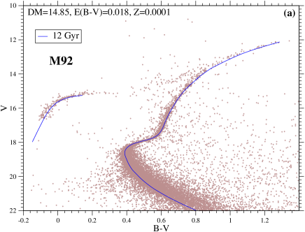
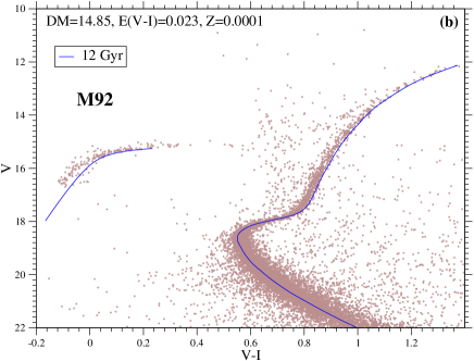
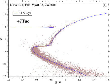
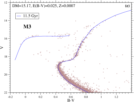
Figure 1: Comparison of present isochrones and CM diagrams for three selected globular clusters, see text. For each cluster the estimated values for age, distance modulus and reddening are labeled together with the metallicity, as calculated from the observed [Fe/H] value (see Sec. 3). Top left and top right panel: comparison for the globular cluster M92, in the $(V,B-V)$ and in the ($V$, $V-I$) diagram, respectively. Bottom right panel: the same, but for the M3 cluster in the ($V$, $B-V$) diagram. Bottom left panel: the same, but for 47 Tuc cluster in the ($V$, $B-V$) diagram.

4 Database description: stellar tracks and Isochrones

Stellar tracks were computed from the PMS phase through the evolution of the whole H and He burning phases up to the first thermal pulse, except for the lowest masses, which take longer than the Hubble time to exhaust the central hydrogen. We covered a range of masses from 0.30 $M_{\sun}$ to 1.10 $M_{\sun}$, in steps of 0.05 $M_{\sun}$. The limit of 0.30 $M_{\sun}$ was chosen because lower masses present along its evolution temperature and pressure value not covered by the OPAL EOS. As shown in Table 1, we selected 19 metallicity values, with $Z$ varying from $Z=0.0001$ to $Z=0.01$.

For each $Z$ value, we computed models with six different helium abundances. Five of them are fixed values ($Y$ = 0.25, 0.27, 0.33, 0.38, 0.42) that simulate different helium enrichments up to the very high values supposed for some stellar samples in multipopulation clusters (Lee et al. 2005; Villanova et al. 2007; Piotto et al. 2007; Piotto 2009), while the last one follows the often adopted linear helium-to-metal enrichment law given by: $Y=Y_{p}+\frac{\Delta Y}{\Delta Z}Z$. For the cosmological ⁴He abundance we adopted the value $Y_{p}=0.2485$, as recently estimated by WMAP (Cyburt et al. 2004; Steigman 2006; Peimbert et al. 2007a, b). For the galactic helium-to-metal enrichment ratio we chose $\Delta Y$/$\Delta Z=2$, a typically assumed value for this quantity that is still affected by several important sources of uncertainty (Pagel & Portinari 1998; Jimenez et al. 2003; Flynn 2004; Gennaro et al. 2010).

We adopted the solar heavy-element mixture recently provided by Asplund et al. (2009). We computed models also for an enhanced abundance of the $\alpha$ elements with respect to the solar mixture with [$\alpha$/Fe] = 0.3 (see e.g. the discussion in Ferraro et al. 1999). Salaris et al. (1993) showed that $\alpha$-enhanced models can be reproduced by the solar-scaled ones with the same total metallicity, provided that the ratio of the high (C, N, O, Ne) over the low (Mg, Si, S, Ca, Fe) ionization potential elements is preserved. However, as pointed out by several authors (see e.g. VandenBerg et al. 2000; Salaris & Weiss 1998; Weiss et al. 1995), this property starts to break down at Z $\approx$ 0.002 and becomes less and less reliable with increasing metallicity.

As already illustrated (see Section 3), the value $\alpha_{ml}=1.90$ was calibrated against the observed CM diagrams of the globular clusters M92, M3 and 47Tuc. However, since the effective temperatures of low-mass stars are considerably affected by changes in the $\alpha_{ml}$ value, we performed calculations also for two other values of the mixing length parameter, $\alpha_{ml}$ = 1.70; 1.80. The solar-calibrated mixing length parameter is $\alpha_{ml}$ = 1.74. The mixing length is merely a fitting parameter, linked to the still unavoidable uncertainties in external convection efficiency calculations. For these reasons the required $\alpha_{ml}$ value could be, in principle, different not only for different stellar masses and chemical compositions, but also for different evolutionary phases of the same model (see e.g. Brocato et al. 1999). Fortunately its influence on model luminosities is quite negligible (see e.g. Chaboyer et al. 1995) for reasonable values of this quantity.

For each set of parameters, two types of track files were included. The first group contains the output of the calculations beginning from the PMS and ending either at the helium flash (for $M\geq 0.55M_{\sun}$) or at central hydrogen exhaustion ($M\leq 0.50M_{\sun}$). The second group, computed for each calculation reaching the helium flash in less than 15 Gyr, consists of files beginning from the zero-age horizontal branch (ZAHB) model and ending at the onset of thermal pulses. Table 1 summarizes the models included in the database. Isochrones were computed in the typical GC age range, from 8 to 15 Gyr, with time steps of 0.5 Gyr. This part of the database therefore contains a total of 11016 tracks starting from PMS, 5549 tracks starting from ZAHB, and 9720 isochrones.

Table 1: Summary of calculated data base tracks (see Sec.4)

Mass range: from 0.30 $M_{\sun}$ to 1.10 $M_{\sun}$, steps of 0.05 $M_{\sun}$
Mixture: Asplund et al. (2009), [$\alpha$/Fe] = 0.0, 0.3
$\alpha_{ml}$ = 1.70, 1.80, 1.90
$Z$	$Y$
0.0001	0.249	0.250	0.270	0.330	0.380	0.420
0.0002	0.249	0.250	0.270	0.330	0.380	0.420
0.0003	0.249	0.250	0.270	0.330	0.380	0.420
0.0004	0.249	0.250	0.270	0.330	0.380	0.420
0.0005	0.250	0.250	0.270	0.330	0.380	0.420
0.0006	0.250	0.250	0.270	0.330	0.380	0.420
0.0007	0.250	0.250	0.270	0.330	0.380	0.420
0.0008	0.250	0.250	0.270	0.330	0.380	0.420
0.0009	0.250	0.250	0.270	0.330	0.380	0.420
0.0010	0.250	0.250	0.270	0.330	0.380	0.420
0.0020	0.252	0.250	0.270	0.330	0.380	0.420
0.0030	0.254	0.250	0.270	0.330	0.380	0.420
0.0040	0.256	0.250	0.270	0.330	0.380	0.420
0.0050	0.258	0.250	0.270	0.330	0.380	0.420
0.0060	0.260	0.250	0.270	0.330	0.380	0.420
0.0070	0.262	0.250	0.270	0.330	0.380	0.420
0.0080	0.264	0.250	0.270	0.330	0.380	0.420
0.0090	0.266	0.250	0.270	0.330	0.380	0.420
0.0100	0.268	0.250	0.270	0.330	0.380	0.420

Track files names were chosen to clearly indicate the inputs used in the simulation. As an example, for $M$ = 0.80 $M_{\sun}$, $Z$ = 0.01, $Y$ = 0.25, $\alpha_{ml}$ = 1.90, solar-scaled Asplund 2009 mixture, the track file from PMS to RGB flash is named OUT_M0.80_Z0.01000_He0.2500_ML1.90_AS09a0.DAT. Outputs starting from ZAHB are named appending the value of ZAHB mass to the name: OUT_M0.80_Z0.01000_He0.2500_ML1.90_AS09a0_ZAHB0.8000.DAT. In each file, the following quantities are listed: model number, age in $\log$ age (yr), luminosity in $\log L/L_{\sun}$, effective temperature in $\log T_{eff}$, central temperature in $\log T_{c}$, central density in $\log\rho_{c}$, mass of the helium core ($M_{He}^{c}/M_{\sun}$), mass of the star ($M_{\sun}$), fractional central abundance in mass of hydrogen (after the H exhaustion: fractional central abundance in mass of He), luminosity of the $pp$ and of the CNO chains, luminosity of the $3\alpha$ burning, luminosity of the gravitational energy, radius of the star ($R_{\sun}$), logarithm of surface gravity. Although in our models the mass is constant, the mass of the evolving star is included to allow a possible future inclusion of mass loss in the database without changing the layout of the output tables. Additional evolutionary quantities for the calculated models are available on request.

Besides the models presented above, a grid of HB models were calculated from an unique RGB progenitor mass for each chemical composition (without mass loss during RGB evolution). This mass was selected to have in RGB an age as close as possible to the mean estimated age value for GCs, i.e. about 12 Gyr. The progenitor masses satisfying this constraint are reported in Table 2; in the most cases the variation of $\alpha$ enhancement and mixing length values does not affect the progenitor mass determination. As is well known, the small dependence of HB characteristics on cluster age can be neglected; a detailed investigation of the age effect on HB models can be found e.g. in Caputo & Cassisi (2002). A total of 16081 models are included in this part of the database.

Lower main-sequence stars ignite helium in a violent flash at the RGB tip; following a common procedure (Dorman et al. 1991; Castellani et al. 1989), instead of modeling this phase, we stopped our calculations of the ZAHB progenitor at the RGB flash, defined as the time when the He burning luminosity reaches 100 times the surface luminosity. The He core mass at this time was assumed as the core mass of the starting models of quiescent central helium burning. In all cases an initial amount of carbon, given by X_C = 0.03, was assumed to be homogeneously distributed throughout the He core, as a product of the He burning during the flash. The chemical composition of the models out to the He core was taken as the external one at the He flash; in this way we also took into account the external helium overabundance with respect to the MS (extra-helium) driven to the surface by the first dredge-up, which also homogenizes the stellar chemical composition out of the He core. Model calculations were therefore started again as thermal relaxed models in the central He burning phase; ZAHB point was fixed when the equilibrium abundance of CNO burning secondary elements was reached, after about 1 Myr. The mass of the H-rich envelope was taken as a free parameter, in dependence on the unknown amount of mass loss experienced in the RGB phase by real cluster stars. In practice, several HB models with fixed He-core mass and external chemical abundance, but different total masses were computed in a way to homogeneously cover the ZAHB extension in effective temperature. We started by creating the first He burning model corresponding to the bluest one. The new model was found by a Runge-Kutta integration (more precisely the “fitting method”, as described in Kippenhahn & Weigert 1994). After creating this model for the lowest mass star, higher mass He burning models, up to one corresponding to the progenitor mass, were calculated by increasing the envelope mass to the required values. During this procedure time steps were artificially kept very short to prevent model evolution.

Comparisons among fully evolved models and horizontal branch models constructed in the described way confirm the reliability of this ZAHB model building procedure (see e.g. Serenelli & Weiss 2005; Piersanti et al. 2004; VandenBerg et al. 2000).

Table 2: Summary of RGB progenitor mass (in $M_{\sun}$) for the computed HB grids.

Mixture: Asplund et al. (2009), [$\alpha$/Fe] = 0.0, 0.3
$\alpha_{ml}$ = 1.70, 1.80, 1.90
$Z$	$Y$
	0.25	0.27	0.33	0.38	0.42
0.0001	0.80	0.75	0.70	0.60	0.55
0.0002	0.80	0.75	0.70	0.60	0.55
0.0003	0.80	0.75	0.70	0.65	0.60
0.0004	0.80	0.75	0.70	0.65	0.60
0.0005	0.80	0.75	0.70	0.65	0.60
0.0006	0.80	0.75	0.70	0.65	0.60
0.0007	0.80	0.80	0.70	0.65	0.60
0.0008	0.80	0.80	0.70	0.65	0.60
0.0009	0.80	0.80	0.70	0.65	0.60
0.001	0.80	0.80	0.70	0.65	0.60
0.002	0.85	0.80	0.70	0.65	0.60
0.003	0.85	0.85	0.75	0.65	0.60
0.004	0.90	0.85	0.75	0.70	0.65
0.005	0.90	0.85	0.75	0.70	0.65
0.006	0.90	0.90	0.80	0.70	0.65
0.007	0.90	0.90	0.80	0.70	0.65
0.008	0.95	0.90	0.80	0.75	0.65
0.009	0.95	0.90	0.80	0.75	0.70
0.01	0.95	0.95	0.85	0.75	0.70

The ZAHB total masses were chosen to span a sizeable range of the ZAHB effective temperature extension: from zero mass loss in RGB (ZAHB mass equal to the progenitor mass) to a mass equal to that of the He core at RGB flash plus a small envelope of 0.026 $M_{\sun}$. The ZAHB models were calculated in intervals of 0.01 $M_{\sun}$ in mass to avoid spurious discontinuities in the ZAHB morphology. Each ZAHB table contains mass in $M_{\sun}$, effective temperature in $\log T_{eff}$ and luminosity in $\log L/L_{\sun}$. The file names were chosen in the same way as the track files: as an example, for $M$ = 0.80 $M_{\sun}$, $Z$ = 0.001, $Y$ = 0.25, $\alpha_{ml}$ = 1.90, solar-scaled Asplund 2009 mixture, the ZAHB file is named ZAHB_M0.80_Z0.00100_He0.2500_ML1.90_AS09a0.DAT.

Isochrones are stored in several directories with self explicative names; as an example the directory ISO_Z0.00100_He0.2500_ML1.90_AS09a0.DAT contains all isochrones with the indicated chemical composition and convection efficiency. The directory hosts several files for the different ages. As an example for a 8.0 Gyr isochrone the file is named AGE08000_Z0.00100_He0.2500_ML1.90_AS09a0.DAT. The header of these files lists the age in Gyr, the $Y$ and $Z$ content, the adopted value for $\alpha_{ml}$ and the solar mixture. The possible $\alpha$ enhancement is specified both in the file name and in the header. For each isochrone the reported quantities are the luminosity in $\log L/L_{\sun}$, the effective temperature in $\log T_{eff}$ and the mass of the star in $M/M_{\sun}$.

Owing to the extremely wide range of possible useful photometric bands and to the dependence of the obtained colors (mainly for cool models) on the adopted color transformations we decided to present results in the theoretical plane only, delaying the presentation of our calculations in several observational planes to a following paper, in which the different sources of uncertainties for theoretical evolutionary models will also be discussed.

Examples of present calculations are shown in Figs. 2 and 3, where tracks and isochrones for $Z=0.001$, $Y=0.25$, $\alpha_{ml}=1.90$ are plotted in the ($\log L/L_{\sun}$, $\log T_{eff}$) plane.

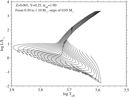
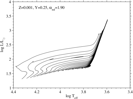
Figure 2: HR diagram for evolutionary tracks in the mass range 0.30 $\div$ 1.10 $M_{\sun}$ for the labeled chemical composition ([$\alpha$/Fe] = 0.0) and $\alpha_{ml}=1.90$. Effective temperatures are in K. Left panel: tracks from PMS up to the central hydrogen exhaustion (for masses up to 0.5 $M_{\sun}$) and tracks from PMS up to the helium flash (for masses $0.55\;M_{\sun}\leq M\leq 1.10\;M_{\sun}$). Right panel: HB models with a 0.80 $M_{\sun}$ progenitor, from the ZAHB to thermal pulses.

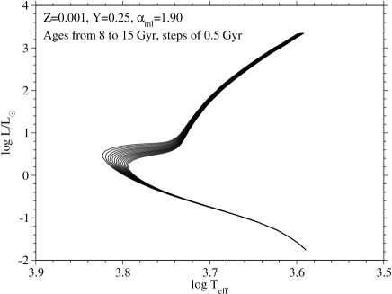
Figure 3: Theoretical isochrones in the range $8\div 15$ Gyr for the labeled chemical compositions with $\alpha_{ml}$ = 1.90 and [$\alpha$/Fe] = 0.0.

5 Comparison with recent stellar model databases

In this section present results for some of the most relevant evolutionary parameters (namely the TO and RGB tip, TRGB, luminosity and the He core mass at the RGB tip, $M_{c}^{He}$) are compared with those of other recent papers available in the literature. As is well known, the TO luminosity is the most important age indicator for globular clusters while tip and horizontal branch luminosity are powerful distance indicators. The TRGB and HB luminosities are proportional to $M_{c}^{He}$ (see e.g. Salaris & Weiss 1998; Buzzoni et al. 1983), which also affects RGB and HB lifetimes.

We selected works that provide an extended database of tracks and isochrones with solar-scaled and $\alpha$-enhanced chemical compositions for the required age range: BaSTI database (Pietrinferni et al. 2004, 2006), Dartmouth (Dotter et al. 2007, 2008), and Padova STEV (Bertelli et al. 2008, 2009). Obviously, the quoted models do not exhaust the rich and composite scenario of stellar evolutionary calculations. Updated stellar models differ in a variety of choices concerning physical inputs and chemical compositions, which produces small but significant changes in the results. Models with physical inputs that differ within the error of each quantity are all acceptable and are useful for estimating the order of magnitude of the uncertainties on the theoretical predictions. The main differences in the inputs of the various codes used by the different authors are summarized in Table 3. From top to bottom we show mass range, metallicity and helium values, the adopted mixture, the $\alpha$ enhancement and the evolutionary phases followed by the models; then we report the adopted mixing length parameter, and the presence or absence of diffusion and overshooting. The following lines list the adopted physical inputs: equation of state (EOS), radiative opacity, nuclear reaction rates, electron conduction in degenerate matter, neutrino energy loss rates. Information about the selected atmospheric model are reported on the last line.

For completeness we notice that our models are suitable for old clusters and therefore they are restricted to lower main-sequence stars which, except for masses of $\approx 1.1$ $M_{\sun}$, have radiative cores; the other quoted databases cover a more extended range of masses including also upper main-sequence stars. Overshooting influences only stars with a mass greater than about 1.1 $M_{\sun}$ (depending on the chemical composition), which start developing small convective cores. Its efficiency is usually modeled to grow linearly with mass, until about 1.5 $\div$ 1.7 $M_{\sun}$. In addition to models computed without overshooting, there are also models in the BaSTI database that adopt a gradual increase of the overshooting efficiency (usually expressed in units of pressure scale height) $\Lambda_{c}=(M/M_{\sun}-0.9)/4$ (Pietrinferni et al. 2004) for $1.1\leq M<1.7\;M_{\sun}$. The Padova database adopts $\Lambda_{c}=M/M_{\sun}-1.0$ (Bertelli et al. 2008) for $1.0<M<1.5M_{\sun}$. In the Dartmouth database the convective core overshooting is linearly increased from 5% of the pressure scale height for $M=M_{min}$ (the value of $M_{min}$ depends on chemical composition and is given in Table 3 of Dotter et al. (2007)), to 20% for $M=M_{min}+0.2\;M_{\sun}$. Above these limits the overshooting efficiency is assumed to be constant. Thus the inclusion of overshooting in the models could slightly influence our comparison only for masses of about 1.1 $M_{\sun}$; in Table 3 we report for each database only the minimum mass in which convective core overshooting is included.

Each database, except the STEV, includes for the chemical composition, models with helium abundance calculated with the quoted linear relation between helium and metal enrichment with a primordial helium abundance of $Y=0.245$ and a relation coefficient of $\approx 1.5\div 2$. Moreover, each database spans a wide range of metallicities and helium abundances; this enabled us to select for our comparison the most similar chemical compositions among those available.

Table 3: Comparison among recent databases.

Models	Present models (Pisa)	BaSTI (Teramo)	STEV(Padova)	Dartmouth
Mass range [$M_{\sun}$]	$0.30\div 1.10$	$0.50\div 10.0$	$0.15\div 20.0$	$0.10\div 4.00$
Metallicity ($Z$)	$1\times 10^{-4}\div 1\times 10^{-2}$	$1\times 10^{-4}\div 4\times 10^{-2}$	$1\times 10^{-4}\div 7\times 10^{-2}$	[Fe/H] = $-2.5\div 0.5$
Helium abundance ($Y$)	0.25; 0.27; 0.33; 0.38; 0.42;	0.245$\leq Y\leq$0.303	0.23; 0.26; 0.30; 0.34;	0.33; 0.40;
	$Y=0.2485+2Z$	$Y=0.245+1.4Z$	0.40; 0.46	$Y=0.245+1.6Z$
Solar mixture	AGSS09	GN93	GN93	GS98
${\rm[}\alpha{\rm/Fe]}$	0.0; +0.3	+0.4	0.0	$-0.2\div+0.8$ ([Fe/H] $\leq 0$)
				$-0.2\div+0.2$ ([Fe/H] $>0$)
Evolutionary phases	PMS; H+He	PMS; H+He	H+He	PMS; H+He
$\alpha_{ml}$	1.70 ; 1.80 ; 1.90	1.913	1.68	1.938
Diffusion	Thoul et al. (1994)	NO	NO	Thoul et al. (1994)
$M_{min}$ for overshoot	NO overshooting	1.1 $M_{\sun}$	1.1 $M_{\sun}$	1.1 $M_{\sun}$
EOS	OPAL2006+Straniero (1988)	FreeEOS	Bertelli et al. (2008)+	Chaboyer & Kim (1995)+
			Mihalas et al. (1990)	FreeEOS
Radiative opacity	OPAL2006+F05	OPAL96+F05	OPAL96+AF94	OPAL96+F05
Conductive opacity	Cassisi et al. (2007)	Potekhin (1999)	Itoh et al. (1983)	Hubbard & Lampe (1969)
		Potekhin et al. (1999)
Reactions rates	NACRE	NACRE	Caughlan & Fowler (1988)	Adelberger et al. (1998)
	Imbriani et al. (2005)			Imbriani et al. (2004)
	Hammer et al. (2005)	Kunz et al. (2002)		Kunz et al. (2002)
	Cyburt & Davids (2008)		Landre et al. (1990)
Neutrinos	Haft et al. (1994)	Haft et al. (1994)	Haft et al. (1994)	Haft et al. (1994)
	Itoh et al. (1996)
Boundary conditions	Brott & Hauschildt (2005)	Krishna Swamy (1966)	Castelli & Kurucz (2003)	Hauschildt et al. (1999)
	Castelli & Kurucz (2003)			Castelli & Kurucz (2003)

We present two comparisons. The first one, in Fig. 4, with $Z=0.004$ and $Y=0.25$, except for the STEV database for which an helium value $Y=0.26$ is available; the effect of this helium variation on the analyzed evolutionary parameters is known to be very small (see e.g. Buzzoni et al. 1983). The second one, in Fig. 5, with $Z=0.008$ and $Y=0.33$, except for the STEV database for which $Y=0.34$ is available; in this case we were unable to select a model from BaSTI with the required $Z$ abundance. The value of $Z=0.004$ and $Z=0.008$ were unavailable in the Dartmouth databases: the isochrones (upper panels in Figs. 4 and 5) were interpolated in $Z$ with a cubic interpolator available on their web site, while the evolutionary quantities (lower panels in Figs. 4 and 5) were interpolated in $Z$ by us with a linear interpolator.

Moreover, there are differences in the solar mixture adopted by the different databases. Recent analysis of spectroscopic data using three dimensional hydrodynamic atmospheric models (see Asplund et al. 2005, 2009) have reduced the derived abundances of CNO and other heavy elements with respect to the previous estimate by Grevesse & Sauval (1998) (hereafter GS98), even if additional investigations are needed (see e.g. Caffau et al. 2009; Socas-Navarro & Norton 2007). If one takes into account the still widely used solar mixture by Grevesse & Noels (1993), with C, N and O abundances slightly higher than those by GS98, the discrepancy with the Asplund et al. (2005, 2009) composition slightly increases. It is worth noticing that uncertainties on the solar mixture have two main effects: a variation of the relation between [Fe/H] and total metallicity $Z$, and a change of the model characteristics at fixed $Z$. For the present comparison at fixed $Z$, we are interested in the second point; fortunately, it is already demonstrated (Degl’Innocenti et al. 2006) that the influence of the adopted mixture on model luminosities and He core mass is very small, while effective temperatures could somehow be affected (see e.g. Salaris et al. 1993).

Figs. 4 and 5 show the results of the comparison among the chosen databases for the isochrone HR diagrams and for the selected evolutionary quantities. For the isochrone comparison we selected the age of 12.5 Gyr because this is a value common to all the databases.

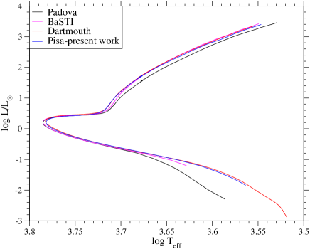
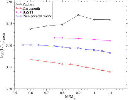
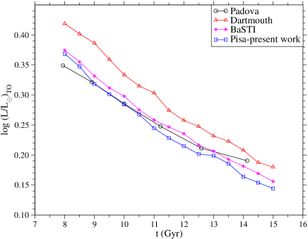
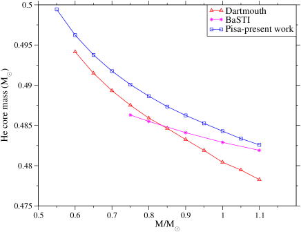
Figure 4: Comparison at $Z=0.004$, $Y=0.25$ and $\alpha_{ml}$ = 1.90 among the different databases of Table 3. For the STEV database, we selected $Y=0.26$ and $\alpha_{ml}$ = 1.68 as the values among those available that are closest to those of the other databases. The tracks of the Dartmouth databases were interpolated in $Z$, see text. Upper left panel: theoretical isochrones at $t$ = 12.5 Gyr. Upper right panel: luminosity at the tip of the red giant branch. Lower left panel: turn-off luminosity. Lower right panel: mass of the helium core at the He flash.

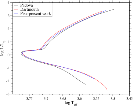
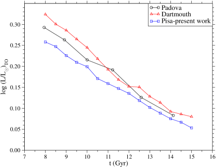
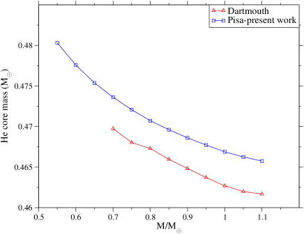
Figure 5: Comparison at $Z=0.008$, $Y=0.33$ and $\alpha_{ml}$ = 1.90 among the different databases of Tab.3. For the STEV database, we selected $Y=0.34$ and $\alpha_{ml}$ = 1.68 as the values among those available that are closest to those of the other databases. The tracks of the Dartmouth databases were interpolated in $Z$, see text. Upper left panel: theoretical isochrones at $t$ = 12.5 Gyr. Upper right panel: red giant branch tip luminosity. Lower left panel: turn-off luminosity. Lower right panel: Helium core mass at the He flash.

As one can see in Table 3, the various databases are computed adopting different choices of the physical inputs; the source of the opacities is quite often the same (except for STEV, which adopts values for low-temperature opacities from Alexander & Ferguson 1994) but the EOS, nuclear reaction rates, boundary conditions and electronic conduction are often different. Moreover, two of the selected databases (Pisa and Dartmouth) are calculated including microscopic diffusion and helium and heavy elements (with the same diffusion coefficients), while the other two databases neglect the diffusion process.

Consequently, a precise quantitative analysis of the differences in the results among the various databases would require the “ad hoc” calculation of several models with different physical inputs, which is beyond the scope of this paper. However, as discussed before, even a more qualitative analysis of the differences is useful to give an indication of the still present uncertainties due to the adoption of different physical inputs in stellar codes.

We did not perform a comparison among the different horizontal branch models because the other databases do not make the corresponding mass grids available.

Elements diffusion occurs on a timescale of a few Gyr, so it influences the main physical characteristics of old clusters only. Diffusion has also been demonstrated to be efficient in the Sun (see e.g. Bahcall et al. 2001; Guzik et al. 2001) for which the huge amount of very precise observational data allow one to observe effects smaller than those occurring in old clusters. The general quoted uncertainty on this process, (see e.g. Thoul et al. 1994), is on the order of 10$\div$15%; however, the treatment of microscopic diffusion still presents several uncertainties even for the Sun for which a very large set of observational data is available (see e.g. Thoul & Montalbán 2007; Montalban et al. 2006; Richer et al. 2000; Turcotte et al. 1998). Surface abundance observations in globular clusters have raised some doubts about the actual efficiency of microscopic diffusion in old cluster stars (see e.g. James et al. 2004; Gratton et al. 2001), but these results seem to not be confirmed by recent analysis (see Korn et al. 2007; Lind et al. 2008, and references therein).

A detailed discussion of the influence of the helium and metal microscopic diffusion on evolutionary properties can be found in Castellani & Degl’Innocenti (1999) (see also Straniero et al. 1997; Castellani et al. 1997). Here we only recall that including microscopic diffusion at a fixed age reduces the TO luminosity by $\Delta\log L/L_{\sun}\approx 0.06$; moreover, He is ignited within a slightly larger He core with a lower He abundance in the envelope, so that the ZAHB luminosity (in the RR Lyrae region at about $\log L/L_{\sun}=3.83$) is slightly decreased, while the TRGB luminosity is almost unaffected (see also Cassisi et al. 1998). The results is that neglecting diffusion leads to an increase of the estimated age through the “vertical method” (Iben & Faulkner 1968) by $\approx$ 1 Gyr.

Another important point is that only two databases adopt the recent value of the ¹⁴N(p,$\gamma$)¹⁵O astrophysical factor by the LUNA Collaboration (Imbriani et al. 2005, and references therein), which is about half of the previous quoted estimates. Some authors (see e.g. Weiss et al. 2005; Imbriani et al. 2004; Degl’Innocenti et al. 2004) analyzed the effects of this cross section update showing that TO luminosity is increased by about 0.03 in $\log L/L_{\sun}$ while the influence on HB luminosity in the RR Lyrae region is a factor three smaller and it also depends on model metallicity; moreover, Pietrinferni et al. (2010) showed that using the LUNA cross section causes an increase of the $M_{c}^{He}$ by about 0.002-0.003 $M_{\sun}$ and a decrease of the TRGB luminosity (because of the lower CNO burning efficiency) of $\Delta\log L/L_{\sun}\approx$ 0.01-0.02 dex.

Selected databases adopt also different, and sometimes not updated, evaluations for conductive opacities that significantly affect the He core mass at the helium ignition, and consequently the HB luminosity (see e.g. Castellani & Degl’Innocenti 1999; Catelan et al. 1996). Castellani & Degl’Innocenti (1999) noticed that the adoption of the Itoh et al. (1983) evaluations, present in the STEV database, instead of the Hubbard & Lampe (1969) ones, adopted by the Dartmouth database, leads to an increase of the helium core of about 0.005 $M_{\sun}$ and thus to a corresponding increase of the ZAHB luminosity by $\Delta\log L/L_{\sun}\approx 0.017$. Moreover, Cassisi et al. (2007) pointed out that the adoption of the Potekhin et al. (1999) conduction opacities provides $M_{c}^{He}$ values between those obtained with the Itoh et al. (1983) and Hubbard & Lampe (1969) ones, but closer to the Itoh et al. (1983) results. In Cassisi et al. (2007) the opacity calculations by Potekhin (1999) and Potekhin et al. (1999) were improved by including the electron-electron scattering in partially degenerate and non degenerate matter. The authors found that the change of the conduction treatment from Potekhin et al. (1999) to Cassisi et al. (2007) leads to a reduction of $M_{c}^{He}$ by about 0.006 $M_{\sun}$ with a corresponding decrease of TRGB luminosity of $\Delta\log L/L_{\sun}\approx 0.03$ and of the ZAHB luminosity by $\Delta\log L/L_{\sun}\approx 0.02$.

From Table 3 one sees that the models belonging to different databases adopt different EOS, hydrogen and helium burning nuclear reaction rates. The result is that the differences among the predicted evolutionary quantities are due to a combination of the effects of all the quoted physical input variations in a way that is difficult to disentangle.

For example, the slightly lower TO luminosity of the present models with respect to the BaSTI ones (see Fig. 4) can be understood in terms of the effects of the diffusion inclusion and of the ¹⁴N(p,$\gamma$)¹⁵ update, taking also into account that the adopted EOS is quite similar and that both databases take most of the reaction rates from NACRE compilation. However, even if present models and Dartmouth calculations adopt the same microscopic diffusion coefficients and ¹⁴N(p,$\gamma$)¹⁵ cross section, TO luminosity differs up to $\Delta\log L/L_{\sun}\approx 0.067$; which is probably at least in part due to the different EOS and H burning reaction rates.

From the isochrone comparison of Figs. 4 and 5, differences in effective temperature appear evident mainly in RGB and in the lower main-sequence. Differences in the RGB location among the various databases are not surprising because its effective temperature is very sensitive to low-temperature opacities, external convection efficiency, and outer boundary conditions. Particularly, the effective temperature of the upper part of the RGB (at luminosity higher than the RGB bump) of the STEV isochrone differs from the others.

There is a fair agreement among the $M_{c}^{He}$ values from the different databases that make this quantity available; the maximum difference is on the order of 0.005 $M_{\sun}$, fully compatible with the adoption of the different physical inputs described above.

All the models, except the STEV, agree within $\Delta\log L/L_{\sun}\approx 0.06$ for the TRGB luminosity; even if it is obvious from the $M_{c}^{He}$ behavior that He core mass is not the only parameter that influences the luminosity at the He flash.

6 Analytical relations

The wide range of chemical compositions spanned by our database and its fine spacing in the input parameters is particularly suitable for the calculation of analytical relations, which express the dependence of the main evolutionary characteristics on the various parameters allowing one to identify the critical input factors for each selected evolutionary feature. Moreover, sufficiently precise enough relations allow one to obtain the required evolutionary results also for a combination of parameters for which models are not directly calculated and can be useful for comparison with other theoretical predictions.

Analytical relations connecting relevant evolutionary quantities with stellar masses and ages can be useful in several fields of stellar evolution, e.g. evolutionary properties of binary systems, synthetic models for simple stellar populations and for star counts in galaxies, chemical evolution models of galaxies (see e.g. Andersen 2002, 1991; Bahcall & Soneira 1980; Chiappini et al. 1997; Bruzual & Charlot 2003; Bruzual A. & Charlot 1993; Haywood 1994; Matteucci 2009; Popper 1997; Hernandez et al. 2000; Portinari & Chiosi 2000; Ribas et al. 2000a, b, for representative works in the quoted fields).

We analyzed two relevant evolutionary features: the TO luminosity and the ZAHB luminosity in the RR Lyrae region.

Analytical computations for the most relevant evolutionary quantities have been published in the past by several authors (see e.g. Carretta et al. 2000; Chaboyer et al. 1998; Cassisi et al. 1998; Buzzoni et al. 1983; Sweigart & Gross 1978, 1976). However, these results were usually restricted to simple linear relations among the evolutionary features of interest and some predictors (or covariates), subsetting data at some fixed values of all other predictors. Although a similar technique produces simple relations, these can not be generalized to other values of the subsetting predictors. In the present work we chose an alternative multivariate approach, allowing the regression models to include not only the predictors but either their interactions. With this choice we were able to fit the whole dataset with the same expression for all the values of predictors. We started with simple relations including linearly the predictors but allowing for interaction between chemical inputs ($Z$ and $Y$) and age (for TO luminosity) or mass of the star. Then we checked whether the model was able to describe all significant trends in the data without over-fitting them (see e.g. Faraway 2004). The first requirement was tackled by the analysis of the standardized residuals, to check that the whole information present in the data was extracted by the model. In this case the plot of standardized residuals versus the values of the evolutionary feature predicted by the model should show the points scattered without a clear path. Moreover, the plots of the standardized residuals versus the predictors were used to infer the need to include quadratic or cubic therms or high-order interactions. The plot of the standardized residuals also allows a visual check of the hypothesis of homoscedasticity, i.e. that the variance of the parent distribution of the residuals remain constant for different values of the covariates – or equivalently for different predicted values. The assessment of the statistical significance of the model covariates are based upon the hypothesis that the parent distribution of the standardized residuals is the standardized normal distribution $N(0,1)$. For a rough check of this hypothesis in the analysis we evaluated the quantile 2.5%, 50% and 97.5% of the standardized residuals and compare them with the corresponding quantile of $N(0,1)$. The problem of possible overfitting requires the use of the stepwise regression (Venables & Ripley 2002) technique, which allows one to evaluate the performance of the multivariate model (balancing the goodness-of-fit and the number of covariates in the model) and of the models nested in this one (i.e. models without some of the covariates). To perform the stepwise model selection we employed the Akaike information criterion (AIC):

$$AIC=n\log\frac{d^{2}_{E}}{n}+2\;p\;,$$

which balances the number of covariates $p$ included in the model and its performance in the data description, measured by the error deviance $d^{2}_{E}$ ($n$ is the number of points in the model). Among the models explored by the stepwise technique we selected that with the lower value of the AIC as the best one.

To describe the model concisely, in this section we used the operator $*$, defined as $A*B\equiv A+B+A\cdot B$, and excluded the presence of the regression coefficients in the models. An expanded version of all regression models is reported in Appendix A.

For the turnoff luminosity we modeled the output of the simulations with the following relation:

$$L_{\rm TO}=t_{9}*(Y+\log Z)+\alpha_{ml}+{\cal K}\;,$$ (1)

where $t_{9}=\log t$ ($t$ is the isochrone age in Gyr), $\alpha_{ml}$ is the mixing length value. Since we explored the effect of only one possible $\alpha$-enhancement on the solar mixture, we chose to model its effect by a categorical dicotomic variable $\cal K$. The model was fitted to the data with a least-squares method using the software R 2.13.1 (R Development Core Team 2011). The coefficients of the fit, along with their statistical significance, are listed in Table 4. In the first two columns of the table we report the least-squares estimates of the regression coefficients and their errors; in the third column we report the $t$-statistic for the tests of the statistical significance of the covariates, and in the fourth column the $p$-values of these tests.

The residual standard error of the fit is $\sigma=0.0088$, so that the fit is fairly accurate in the description of the data. The diagnostic plot of standardized residuals of the fit versus predicted values is shown in Fig. 6, panel (a); it is apparent that Eq. 1 gives a good analytical description of the data. The effect of the $\alpha$-enhancement, although statistically significant, is very small – about 0.0019 dex – and may be safely neglected without modification in the model.

We calibrated of the ZAHB luminosity taken at $\log T_{eff}=3.83$ in the central region of the RR Lyrae instability strip. The luminosity was obtained by a linear interpolation in $\log T_{eff}$ on the ZAHB grid. We modeled the luminosity $L_{\rm HB-T3.83}$ with the following function of the mass of the star, the helium and the metal content:

$$L_{\rm HB-T3.83}=(M+M^{2})*Y+\log Z\;,$$ (2)

where $M$ (in $M_{\sun}$) is the mass of the star.

However, the least-squares fit suffers of a heteroscedasticity problem because the plot of standardized residuals (not shown here) has a fan-shaped behavior, showing an increase of the variance with the mass of the star. We modeled this increase with a power law in the mass, $\sigma\propto M^{\beta}$, and corrected the eteroscedasticity by a weighted least-squares fit. Through restricted maximum likelihood techniques we estimated the model coefficients and the power $\beta$ that models the variance trend. We performed the fit with the gls function of the nlme library (Pinheiro et al. 2011) of the R software. The model result is presented in Table 5. The residual standard error of the fit is $\sigma=0.032$, with $\beta=2.05$ (95% confidence interval = [1.54, 2.55]). The diagnostic plot in Fig. 6, panel (b) shows that the data are adequately described by the model.

Table 4: Fit of the turnoff luminosity. In the first two columns: least-squares estimates of the regression coefficients and their errors; third column: $t$-statistic for the tests of the statistical significance of the covariates; fourth column: $p$-values of the tests. The residual standard error is $\sigma=0.0088$.

	Estimate	Std. Error	$t$ value	$p$ value
(Intercept)	0.5964	0.008732	68.31	$<2\times 10^{-16}$
$t_{9}$	-0.4972	0.008026	-61.95	$<2\times 10^{-16}$
$Y$	-1.150	0.01870	-61.53	$<2\times 10^{-16}$
$\log Z$	-0.3125	0.002006	-155.80	$<2\times 10^{-16}$
$\alpha_{ml}$	0.03503	0.001165	30.07	$<2\times 10^{-16}$
$\cal K$ = AS09a3	0.001896	0.0001902	9.97	$<2\times 10^{-16}$
$t_{9}\cdot Y$	0.3158	0.01770	17.84	$<2\times 10^{-16}$
$t_{9}\cdot\log Z$	0.1731	0.001899	91.18	$<2\times 10^{-16}$

Table 5: Fit of HB luminosity taken at $\log T_{eff}=3.83$. The residual standard error is $\sigma=0.032$. The column legend is the same as Table 4.

	Estimate	Std. Error	$t$ value	$p$ value
(Intercept)	$-1.438$	$0.4548$	$-3.163$	$1.7\times 10^{-3}$
$M$	$5.935$	$1.136$	$5.224$	$2.7\times 10^{-7}$
$M^{2}$	$-3.481$	$0.7425$	$-4.688$	$3.7\times 10^{-6}$
$Y$	$6.247$	$1.283$	$4.870$	$1.6\times 10^{-6}$
$\log Z$	$-0.1067$	$0.004814$	$-22.17$	$<2\times 10^{-16}$
$M\cdot Y$	$-11.14$	$3.491$	$-3.190$	$1.5\times 10^{-3}$
$M^{2}\cdot Y$	$5.844$	$2.441$	$2.394$	$1.7\times 10^{-2}$

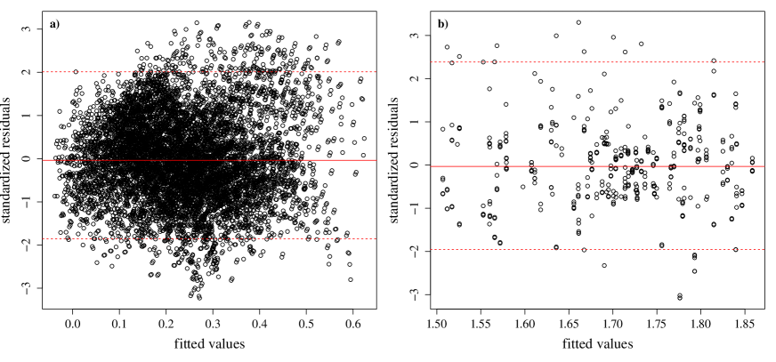
Figure 6: Diagnostic plots showing standardized residuals of the fits versus predicted values. Panel (a): $L_{\rm TO}$; panel (b): $L_{\rm HB-T3.83}$. The dashed lines show the location of the quantiles 2.5% and 97.5% of the standardized residuals, while the solid one shows their median value.

7 Conclusions

We presented a very large set of new stellar tracks and isochrones computed with an updated version of the FRANEC code, which includes state-of-the-art input physics (radiative and conductive opacity, equation of state, atmospheric models and nuclear cross-sections). The main novelties of these models with respect to those currently available in the literature are the adoption of the heavy-element solar mixture by Asplund et al. (2009), the recent ${}^{14}N(p,\gamma)^{15}O$ reaction rate by Imbriani et al. (2005), and the boundary conditions from detailed atmosphere models.

With the aim to provide a powerful and versatile tool for the interpretation of the unceasingly growing amount of data, we computed a very large database covering a fine grid of masses, ages, and chemical compositions. More specifically, in the mass range $0.30\div 1.10$ $M_{\sun}$, we made evolutionary tracks and isochrones for 19 metallicities available, ranging from $Z$ = 0.0001 to 0.01, and five different helium abundances for each $Z$ ranging from $Y$ = 0.25 to 0.42. The availability of sets of models with initial helium abundance as high as 0.33, 0.38, and 0.42 is of primary importance in the context of multipopulation globular cluster studies. For each choice of initial metallicity $Z$ and helium abundance $Y$, we computed tracks and isochrones with two different element mixtures, namely solar-scaled by Asplund et al. (2009) and $\alpha$-enhanced with [$\alpha$/Fe] = 0.3. Finally, we provided all these sets of models for three different values of the mixing-length parameter $\alpha_{ml}$ = 1.70, 1.80, and 1.90. Each set contains evolutionary tracks from the pre-MS to the helium flash, HB models, and isochrones in the age range $8\div 15$ Gyr, in time steps of 0.5 Gyr.

The database, currently consisting of about 33000 stellar tracks and about 10000 isochrones, is available on the web.

Models were compared with other computations available in the literature and with data of selected globular clusters.

We also provided useful analytical relations describing the dependence of relevant evolutionary quantities, namely turn-off and horizontal branch luminosities, on the chemical composition and convection efficiency. More important, we analyzed these relations for the first time in a thorough statistical way to obtain simple but accurate models and to shed some light on the interesting interactions of the chemical and physical inputs of the simulations.

Appendix A Full form of the regression models

The full form of the proposed model for the TO luminosity is

$$L_{\rm TO} = \beta_{0}+\beta_{1}\;t_{9}+\beta_{2}\;Y+\beta_{3}\;\log Z+\beta_{4}\;\alpha_{ml}+\beta_{5}\;{\cal K}+$$ (3)

$$+ \beta_{6}\;t_{9}\cdot Y+\beta_{7}\;t_{9}\cdot\log Z\;,$$

the regression coefficients $\beta_{i}$ are listed in the same order as in Table 4.

The full form of the model of the luminosity $L_{\rm HB-T3.83}$ is

$$L_{\rm HB-T3.83} = \beta_{0}+\beta_{1}\;M+\beta_{2}\;M^{2}+\beta_{3}\;Y+\beta_{4}\;\log Z+$$ (4)

$$+ \beta_{5}\;M\cdot Y+\beta_{6}\;M^{2}\cdot Y\;,$$

the regression coefficients $\beta_{i}$ are listed in the same order as in Table 5.