Exclusive $c\to s,d$ semileptonic decays of ground-state spin-1/2 and spin-3/2 doubly heavy $cb$ baryons

Abstract

We evaluate exclusive semileptonic decays of ground-state spin-1/2 and spin-3/2 doubly heavy $cb$ baryons driven by a $c\to s,d$ transition at the quark level. We check our results for the form factors against heavy quark spin symmetry constraints obtained in the limit of very large heavy quark masses and near zero recoil. Based on those constraints we make model independent, though approximate, predictions for ratios of decay widths.

I Introduction

In this work we make a systematic analysis of exclusive semileptonic $c\to s,d$ decays of doubly heavy ground state $cb$ baryons. Previous studies are very limited and, to our knowledge, they only include the work in Ref. sanchis95 where the $\Xi^{\prime}_{cb}\to\Xi_{b}$ decay was analyzed using heavy quark spin symmetry, the relativistic three quark model calculation of the $\widehat{\Xi}_{cb}\to\Xi^{\prime}_{b}$ decay in Ref. Faessler:2001mr , and the combined branching ratio for the $(\Xi_{cb}\to\Xi_{b})+(\Xi_{cb}\to\Xi^{\prime}_{b})+(\Xi_{cb}\to\Xi^{*}_{b})$ decay evaluated in Ref. Kiselev:2001fw in the framework of the potential approach and QCD sum rules. Since the modulus of the Cabbibo-Kobayashi-Maskawa (CKM) matrix elements $|V_{cs}|,\,|V_{cd}|$ are much larger than $|V_{cb}|$, one would expect the decay widths for $c\to s,d$ semileptonic decay of $cb$ baryons to be much larger than the corresponding $b\to c$ driven decays which have been more extensively studied in the literature sanchis95 ; Ebert:2004ck ; Hernandez:2007qv ; pervin2 ; Faessler:2009xn ; Albertus:2009ww . However, this is corrected by a smaller available phase space, and the decay widths for $c\to s$ transitions turn out to be larger but of the same order of magnitude as the $b\to c$ decay widths, while widths for $c\to d$ transitions are much smaller. In any case, the analysis of the $c\to s,d$ decays of $cb$ baryons could give relevant information on heavy quark physics complementary to the one obtained from the study of the $b\to c$ decays.

Similar to what happens in atomic physics, in hadrons with a single heavy quark the dynamics of the light degrees of freedom becomes independent of the heavy quark flavor and spin when the mass of the heavy quark is much larger than $\Lambda_{QCD}$ and the masses and momenta of the light quarks. This is the essence of heavy quark symmetry (HQS) hqs1 ; hqs2 ; hqs3 ; hqs4 . HQS guaranties that in a heavy baryon the light degrees of freedom quantum numbers are well defined. Then, up to corrections in the inverse of the heavy quark mass, one can take the spin of the two light quarks to be well defined. The two light quarks couple to a state with spin $S=$0 or 1 and then couple with the $b$ quark to total spin 1/2 or 3/2. This is the classification scheme followed for the $b$ heavy baryons in Table 1. However, HQS can not be applied to hadrons containing two heavy quarks. There, the kinetic energy term needed to regulate infrared divergences breaks the heavy quark flavor symmetry, but not the spin symmetry for each heavy quark flavor thacker91 . This is known as heavy quark spin symmetry (HQSS). According to HQSS Jenkins:1992nb , for large heavy quark masses one can select the heavy quark subsystem of a doubly heavy baryon to have a well defined total spin. Again this is the classification scheme followed for $cb$ states shown in Table 1. There, the $c$ and $b$ quark couple to a state with spin $S=$0 or 1 and then couple with the light quark to total spin 1/2 or 3/2. Being the heavy quark masses finite, one has that for spin-1/2 baryons the hyperfine interaction can admix both $S=$0 and $S$=1 components into the wave function of physical states. As shown in Sec. II this is very relevant for spin-1/2 $cb$ baryons. In principle one should also expect some degree of mixing for the $\Xi_{b}$ and $\Xi^{\prime}_{b}$ states. However, in this latter case the hyperfine matrix elements responsible for mixing are proportional to the inverse of the $b$ quark mass and mixing effects are thus suppressed.

In Table 1 we present the baryons involved in the present study. As mention the $\Xi_{cb},\Xi^{\prime}_{cb}$ and $\Omega_{cb},\Omega^{\prime}_{cb}$ are not the physical states that will be discussed in the following. The quark model masses in Table 1 have been taken from our previous works in Refs. Albertus:2003sx ; Albertus:2009ww , where they were obtained using the AL1 potential of Refs. semay94 ; silvestre96 . Experimental masses are the ones given by the particle data group (PDG) in Ref. pdg10 and in the table we quote the average over the different charge states. The agreement with our results is better than 1%. For the actual calculation of the decay widths we shall use experimental masses taken from Ref. pdg10 whenever possible. For the neutral $\Sigma^{*\,0}_{b}$ state we follow Ref. hwang07 and take $M_{\Sigma_{b}^{*\,0}}=\frac{1}{2}(M_{\Sigma_{b}^{*\,+}}+M_{\Sigma_{b}^{*\,-}})$. For the $\Sigma_{b}^{0}$ case, corrections to the analogous relation, due to the electromagnetic interaction between the two light quarks in the heavy baryon, have been evaluated in Ref. Hwang:2008dj using heavy quark effective theory and in Ref. Guo:2008ns in chiral perturbation theory to leading one-loop order. Based on the known experimental data they get $M_{\Sigma_{b}^{0}}=5810.5\pm 2.2\,$MeV Hwang:2008dj and $M_{\Sigma_{b}^{0}}=5810.3\pm 1.9\,$MeV Guo:2008ns , their central values being 1 MeV lower than the value one would obtain from the less accurate relation $M_{\Sigma_{b}^{\,0}}=\frac{1}{2}(M_{\Sigma_{b}^{\,+}}+M_{\Sigma_{b}^{\,-}})$. Here we shall use the value $M_{\Sigma_{b}^{0}}=5810.5\,$MeV given in Ref. Hwang:2008dj . For the $\Xi^{\prime}_{b},\Xi^{*}_{b},\Omega^{*}_{b}$ we take our predictions in Ref. Albertus:2003sx which are in agreement with lattice results by the UKQCD Collaboration ukqcd96 . For doubly heavy $cb$ baryons baryons there is no experimental information on their masses and we shall use our own predictions in Ref. Albertus:2009ww .

Baryon	$J^{P}$	$I$	$S^{\pi}$	Quark content	Mass [MeV]
					Quark model	Experiment
					Albertus:2003sx ; Albertus:2009ww	pdg10
$\Xi_{cb}$	$\frac{1}{2}^{+}$	$\frac{1}{2}$	$1^{+}$	$cbn$	6928	–
$\Xi^{\prime}_{cb}$	$\frac{1}{2}^{+}$	$\frac{1}{2}$	$0^{+}$	$cbn$	6958	–
$\Xi^{*}_{cb}$	$\frac{3}{2}^{+}$	$\frac{1}{2}$	$1^{+}$	$cbn$	6996	–
$\Omega_{cb}$	$\frac{1}{2}^{+}$	0	$1^{+}$	$cbs$	7013	–
$\Omega^{\prime}_{cb}$	$\frac{1}{2}^{+}$	0	$0^{+}$	$cbs$	7038	–
$\Omega^{*}_{cb}$	$\frac{3}{2}^{+}$	0	$1^{+}$	$cbs$	7075	–
$\Lambda_{b}$	$\frac{1}{2}^{+}$	0	$0^{+}$	$udb$	5643	$5620.2\pm 1.6$
$\Sigma_{b}$	$\frac{1}{2}^{+}$	1	$1^{+}$	$nnb$	5851	$5811.5\pm 2.4$
$\Sigma^{*}_{b}$	$\frac{3}{2}^{+}$	1	$1^{+}$	$nnb$	5882	$5832.7\pm 3.1$
$\Xi_{b}$	$\frac{1}{2}^{+}$	$\frac{1}{2}$	$0^{+}$	$nsb$	5808	$5790.5\pm 2.7$
$\Xi^{\prime}_{b}$	$\frac{1}{2}^{+}$	$\frac{1}{2}$	$1^{+}$	$nsb$	5946	–
$\Xi^{*}_{b}$	$\frac{3}{2}^{+}$	$\frac{1}{2}$	$1^{+}$	$nsb$	5975	–
$\Omega_{b}$	$\frac{1}{2}^{+}$	0	$1^{+}$	$ssc$	6033	$6071\pm 40$
$\Omega^{*}_{b}$	$\frac{3}{2}^{+}$	0	$1^{+}$	$ssc$	6063	–

Table 1: Quantum numbers of baryons involved in this study. For the $cb$ baryons, states with a well defined spin for the heavy subsystem are shown. $J^{\pi}$ and $I$ are the spin-parity and isospin of the baryon, while $S^{\pi}$ is the spin-parity of the two heavy or the two light quark subsystem. $n$ denotes a $u$ or $d$ quark. Experimental masses are isospin averaged over the values reported by the PDG pdg10 .

The paper is organized as follows: in Sec II we discuss the physical spin-1/2 $cb$ baryons and the relevance of hyperfine mixing for those states. In Sec. III we give general formulas needed to compute the semileptonic decay width, we present the form factor decompositions that we use for the different transitions and we present and discuss our predictions for the $c\to s,d$ decay widths. In Sec. IV we obtain HQSS constraints for the form factors and make predictions for ratios of decay widths based on those constraints. Finally in Sect. V, we summarize the main results of this work. The paper contains also two appendices. In appendix A we present our nonrelativistic baryon states, while in appendix B we give details on how we evaluate the transition matrix elements and form factors.

II Configuration mixing in $cb$ doubly heavy baryons

Due to the finite value of the heavy quark masses, the hyperfine interaction between the light quark and any of the heavy quarks can admix both $S$=0 and 1 components into the wave function for total spin-1/2 states. Thus, the actual physical spin-1/2 $cb$ baryons are admixtures of the $\Xi_{cb},\,\Xi^{\prime}_{cb}$ ($\Omega_{cb},\,\Omega^{\prime}_{cb}$) states listed in Table 1. The physical states, that we shall call $\Xi_{cb}^{(1)},\,\Xi_{cb}^{(2)}$ and $\Omega_{cb}^{(1)},\,\Omega_{cb}^{(2)}$, are given within the AL1 model by Albertus:2009ww

$$\Xi_{cb}^{(1)} = -0.902\ \Xi^{\prime}_{cb}+0.431\ \Xi_{cb}\ \ ;\ M_{\Xi_{cb}^{(1)}}=6967\,{\rm MeV},$$

$$\Xi_{cb}^{(2)} = \hskip 7.11317pt0.431\ \Xi^{\prime}_{cb}+0.902\ \Xi_{cb}\ \ ;\ M_{\Xi_{cb}^{(2)}}=6919\,{\rm MeV},$$ (1)

$$\Omega_{cb}^{(1)} = -0.899\ \Omega^{\prime}_{cb}+0.437\ \Omega_{cb}\ \ ;\ M_{\Omega_{cb}^{(1)}}=7046\,{\rm MeV},$$

$$\Omega_{cb}^{(2)} = \hskip 7.11317pt0.437\ \Omega^{\prime}_{cb}+0.899\ \Omega_{cb}\ \ ;\ M_{\Omega_{cb}^{(2)}}=7005\,{\rm MeV},$$ (2)

Comparing the masses of the physical states with the mass values quoted in Table 1, one sees that masses are not very sensitive to hyperfine mixing. On the other hand, it was pointed out by Roberts and Pervin pervin1 that hyperfine mixing could greatly affect the decay widths of doubly heavy $cb$ baryons. This assertion was checked in Ref. pervin2 where Roberts and Pervin found that hyperfine mixing in the $cb$ states has a tremendous impact on doubly heavy baryon $b\to c$ semileptonic decay widths. These results were qualitatively confirmed by our own calculation in Ref. Albertus:2009ww . We further investigated the role of hyperfine mixing in electromagnetic transitions Albertus:2010hi finding again large corrections to the decay widths. A similar study was conducted by Branz et al. in Ref. Branz:2010pq . We expect configuration mixing should also play an important role for $c\to s,d$ semileptonic decay of $cb$ baryons.

One way of minimizing the hyperfine mixing for $cb$ baryons is to use from the start baryon states in which the $c$ quark and the light $q$ quark couple to a state of well defined spin $S_{cq}=0$ or 1. Then the $b$ quark couples to that state to make the baryon with total spin 1/2. We denote those states as $\widehat{\Xi}_{cb},\,\widehat{\Omega}_{cb}$ for $S_{cq}=1$, and $\widehat{\Xi}^{\prime}_{cb},\,\widehat{\Omega}^{\prime}_{cb}$ for $S_{cq}=0$. The relation between the latter set of states and the ones in Table 1 is given by (here $B$ stands for $\Xi$ or $\Omega$)

$$\widehat{B}_{cb} = -\frac{\sqrt{3}}{2}B^{\prime}_{cb}+\frac{1}{2}B_{cb},$$

$$\widehat{B}^{\prime}_{cb} = \frac{1}{2}B^{\prime}_{cb}+\frac{\sqrt{3}}{2}B_{cb}.$$ (3)

Hyperfine mixing for the $\widehat{B}_{cb},\,\widehat{B}^{\prime}_{cb}$ states is much less important since it is inversely proportional to the $b$ quark mass Albertus:2009ww . Physical spin-1/2 $cb$ baryons states should then be very close to the $\widehat{B}_{cb},\,\widehat{B}^{\prime}_{cb}$ states and this is indeed the case. If we write

$$\left(\begin{array}[]{c}B^{(1)}_{cb}\vspace{.1cm}\\ B^{(2)}_{cb}\end{array}\right)=\left(\begin{array}[]{cc}\cos\theta&\sin\theta\\ -\sin\theta&\cos\theta\end{array}\right)\left(\begin{array}[]{c}\widehat{B}_{cb}\\ \widehat{B}^{\prime}_{cb}\end{array}\right)$$ (10)

we find $\theta_{\Xi}=-4.46^{o},\ \theta_{\Omega}=-4.07^{o}$ for the AL1 interquark interaction Albertus:2009ww .

III Semileptonic decay widths

III.1 General formulas

The total decay width for semileptonic $c\to l$ transitions, with $l=s,d$, is given by

$$\Gamma = |V_{cl}|^{2}\frac{G_{F}^{\,2}}{8\pi^{4}}\frac{M^{\prime 2}}{M}\int\sqrt{\omega^{2}-1}\,{\cal L}^{\alpha\beta}(q){\cal H}_{\alpha\beta}(P,P^{\prime})\,d\omega,$$ (11)

where $|V_{cl}|$ is the modulus of the corresponding CKM matrix element for a semileptonic $c\to l$ decay ($|V_{cs}|=0.97345$ and $|V_{cd}|=0.2252$ pdg10 ), $G_{F}=1.16637(1)\times 10^{-11}$ MeV^-2 pdg10 is the Fermi decay constant, $P,M$ ($P^{\prime},M^{\prime}$) are the four-momentum and mass of the initial (final) baryon, $q=P-P^{\prime}$ and $\omega$ is the product of the initial and final baryon four-velocities $\omega=v\cdot v^{\prime}=\frac{P}{M}\cdot\frac{P^{\prime}}{M^{\prime}}=\frac{M^{2}+M^{\prime 2}-q^{2}}{2MM^{\prime}}$. In the decay, $\omega$ ranges from $\omega=1$, corresponding to zero recoil of the final baryon, to a maximum value that, neglecting the neutrino mass, is given by $\omega=\omega_{\rm max}=\frac{M^{2}+M^{\prime 2}-m^{2}}{2MM^{\prime}}$, which depends on the transition and where $m$ is the final charged lepton mass. Finally ${\cal L}^{\alpha\beta}(q)$ is the leptonic tensor after integrating in the lepton momenta. It can be cast as

$${\cal L}^{\alpha\beta}(q)=A(q^{2})\,g^{\alpha\beta}+B(q^{2})\,\frac{q^{\alpha}q^{\beta}}{q^{2}},$$ (12)

where explicit expressions for the scalar functions $A(q^{2})$ and $B(q^{2})$ can be found in Eqs. (3) and (4) of Ref. Albertus:2011xz .

The hadron tensor ${\cal H}_{\alpha\beta}(P,P^{\prime})$ is given by

$${\cal H}^{\alpha\beta}(P,P^{\prime}) = \frac{1}{2J+1}\sum_{r,r^{\prime}}\big{\langle}B^{\prime},r^{\prime}\ \vec{P}^{\,\prime}\big{|}J_{cl}^{\alpha}(0)\big{|}B,r\ \vec{P}\big{\rangle}\ \big{\langle}B^{\prime},r^{\prime}\ \vec{P}^{\,\prime}\big{|}J_{cl}^{\beta}(0)\big{|}B,r\ \vec{P}\big{\rangle}^{*},$$ (13)

with $J$ the initial baryon spin, $\big{|}B,r\ \vec{P}\big{\rangle}\,\left(\big{|}B^{\prime},r^{\prime}\ \vec{P}\,^{\prime}\big{\rangle}\right)$ the initial (final) baryon state with three-momentum $\vec{P}$ ($\vec{P}\,^{\prime}$) and spin third component $r$ ($r^{\prime}$) in its center of mass frame. Our states are constructed in appendix A. Finally, $J_{cl}^{\mu}(0)=\bar{\Psi}_{l}(0)\gamma^{\mu}(1-\gamma_{5})\Psi_{c}(0)$ is the $c\to l$ charged weak current.

III.2 Form factors for $1/2\to 1/2$, $1/2\to 3/2$ and $3/2\to 1/2$ transitions

For the actual calculation of the decay width we parametrize the hadronic matrix elements in terms of form factors, which are functions of $\omega$ or equivalently of $q^{2}$. The different form factor decomposition that we use are given in the following.

1. $\ 1/2\to 1/2$ transitions.
   Here we take the commonly used decomposition in terms of three vector $F_{1},\,F_{2},\,F_{3}$ and three axial $G_{1},\,G_{2},\,G_{3}$ form factors

   $$\big{\langle}B^{\prime}(1/2),r^{\prime}\ \vec{P}^{\,\prime}\left|\,J_{cl}^{\mu}(0)\right|B(1/2),r\ \vec{P}\big{\rangle} = {\bar{u}}^{B^{\prime}}_{r^{\prime}}(\vec{P}^{\,\prime})\Big{\{}\gamma^{\mu}\left[F_{1}(\omega)-\gamma_{5}G_{1}(\omega)\right]+v^{\mu}\left[F_{2}(\omega)-\gamma_{5}G_{2}(\omega)\right]$$ (15)

   $$\hskip 42.67912pt+v^{\prime\mu}\left[F_{3}(\omega)-\gamma_{5}G_{3}(\omega)\right]\Big{\}}u^{B}_{r}(\vec{P}\,).$$

   The $u_{r}$ are Dirac spinors normalized as $({u}_{r^{\prime}})^{\dagger}u_{r}=2E\,\delta_{rr^{\prime}}$.

2. $\ 1/2\to 3/2$ transitions.
   In this case we follow Llewellyn Smith Llewellyn Smith:1971zm to write

   $$\big{\langle}B^{\prime}(3/2),r^{\prime}\vec{P}^{\prime}\,|\,\overline{\Psi}_{l}(0)\gamma^{\mu}(1-\gamma_{5})\Psi_{c}(0)\,|\,B(1/2),r\,\vec{P}\,\big{\rangle}=~{}\bar{u}^{B^{\prime}}_{\lambda\,r^{\prime}}(\vec{P}\,^{\prime})\,\Gamma^{\lambda\mu}(P,P^{\prime})\,u^{B}_{r}(\vec{P}\,),$$

   $$\Gamma^{\lambda\mu}(P,P^{\prime})= \left[\frac{C_{3}^{V}}{M}(g^{\lambda\,\mu}q/\,-q^{\lambda}\gamma^{\mu})+\frac{C_{4}^{V}}{M^{2}}(g^{\lambda\,\mu}q\cdot P^{\prime}-q^{\lambda}P^{\prime\mu})+\frac{C_{5}^{V}}{M^{2}}(g^{\lambda\,\mu}q\cdot P-q^{\lambda}P^{\mu})+C_{6}^{V}g^{\lambda\,\mu}\right]\gamma_{5}$$ (16)

   $$+\left[\frac{C_{3}^{A}}{M}(g^{\lambda\,\mu}q/\,-q^{\lambda}\gamma^{\mu})+\frac{C_{4}^{A}}{M^{2}}(g^{\lambda\,\mu}q\cdot P^{\prime}-q^{\lambda}P^{\prime\mu})+{C_{5}^{A}}g^{\lambda\,\mu}+\frac{C_{6}^{A}}{M^{2}}q^{\lambda}q^{\mu}\right].$$

   Here $u^{B^{\prime}}_{\lambda\,r^{\prime}}$ is the Rarita-Schwinger spinor of the final spin 3/2 baryon normalized such that $(u_{\lambda\,r^{\prime}}^{B^{\prime}})^{\dagger}u^{B^{\prime}\,\lambda}_{r}=-2E^{\prime}\,\delta_{rr^{\prime}}$, and we have four vector ($C^{V}_{3,4,5,6}(\omega)$) and four axial ($C^{A}_{3,4,5,6}(\omega)$) form factors. Within our model we shall have that $C^{V}_{5}(\omega)=C^{V}_{6}(\omega)=C^{A}_{3}(\omega)=0$.

3. $3/2\to 1/2$ transitions.
   Similar to the case before we use

   $$\left\langle B^{\prime}(1/2),r^{\prime}\ \vec{P}^{\,\prime}\left|\,\overline{\Psi}_{l^{\prime}}(0)\gamma^{\mu}(1-\gamma_{5})\Psi_{c}(0)\right|B(3/2),r\ \vec{P}\right\rangle=(\bar{u}^{B}_{\lambda\,r}(\vec{P}\,)\tilde{\Gamma}^{\lambda\,\mu}(P^{\prime},P)u^{B^{\prime}}_{r^{\prime}}(\vec{P}\,^{\prime}))^{*}$$

   $$\hskip 192.05609pt=\bar{u}^{B^{\prime}}_{r^{\prime}}(\vec{P}\,^{\prime})\gamma^{0}(\tilde{\Gamma}^{\lambda\,\mu}(P^{\prime},P))^{\dagger}\gamma^{0}{u}^{B}_{\lambda\,r}(\vec{P}),$$

   $$\tilde{\Gamma}^{\lambda\,\mu}(P^{\prime},P)= \left(-\frac{C_{3}^{V}(\omega)}{M^{\prime}}(g^{\lambda\,\mu}q/\,-q^{\lambda}\gamma^{\mu})-\frac{C_{4}^{V}(\omega)}{M^{\prime 2}}(g^{\lambda\,\mu}q\cdot P-q^{\lambda}P^{\mu})-\frac{C_{5}^{V}(\omega)}{M^{\prime 2}}(g^{\lambda\,\mu}q\cdot P^{\prime}-q^{\lambda}P^{\prime\mu})+C_{6}^{V}(\omega)g^{\lambda\,\mu}\right)\gamma_{5}$$ (17)

   $$+\left(-\frac{C_{3}^{A}(\omega)}{M^{\prime}}(g^{\lambda\,\mu}q/\,-q^{\lambda}\gamma^{\mu})-\frac{C_{4}^{A}(\omega)}{M^{\prime 2}}(g^{\lambda\,\mu}q\cdot P-q^{\lambda}P^{\mu})+{C_{5}^{A}(\omega)}g^{\lambda\,\mu}+\frac{C_{6}^{A}(\omega)}{M^{\prime 2}}q^{\lambda}q^{\mu}\right).$$

   Again, and within our model, we shall have that $C^{V}_{5}(\omega)=C^{V}_{6}(\omega)=C^{A}_{3}(\omega)=0$.

4. $\ 3/2\to 3/2$ transitions.
   A form factor decomposition for $3/2\to 3/2$ can be found in Ref. Faessler:2009xn where a total of 7 vector plus 7 axial form factors are needed. In this case we do not evaluate the form factors but work directly with the vector and axial matrix elements.

In appendix B we give the expressions that relate the form factors to weak current matrix elements and show how the latter ones are evaluated in the model. Relations found between matrix elements that simplify the calculation are also shown there.

III.3 Results

The results we obtain for the semileptonic decay widths of $cb$ baryons are presented in Tables 2 ($c\to s$ decays) and 3 ($c\to d$ decays). We show between parentheses the results obtained ignoring configuration mixing in the spin-1/2 $cb$ initial baryons. In this latter case, the $\Xi^{(1)}_{cb},\ \Xi^{(2)}_{cb}$ baryons should be interpreted respectively as the $\Xi^{\prime}_{cb},\ \Xi_{cb}$ states of Table 1. We see small changes for transitions to final states where the two light quarks couple to spin 0. On the other hand, configuration mixing effects are very important for transitions to final states where the two light quarks couple to spin 1, where we find enhancements or reductions as large as a factor of 2.

	$\Gamma\ [10^{-14}\,{\rm GeV}]$
	This work	sanchis95	Faessler:2001mr	Kiselev:2001fw
$\Xi^{(1)\,+}_{cbu}\to\Xi^{0}_{b}\,e^{+}\nu_{e}$	3.74 (3.45)	(3.4)
$\Xi^{(2)\,+}_{cbu}\to\Xi^{0}_{b}\,e^{+}\nu_{e}$	2.65 (2.87)
$\Xi^{(1)\,+}_{cbu}\to\Xi^{\prime 0}_{b}\,e^{+}\nu_{e}$	3.88 (1.66)		$2.44\div 3.28^{\dagger}$
$\Xi^{(2)\,+}_{cbu}\to\Xi^{\prime 0}_{b}\,e^{+}\nu_{e}$	1.95 (3.91)
$\Xi^{(1)\,+}_{cbu}\to\Xi^{*\,0}_{b}\,e^{+}\nu_{e}$	1.52 (3.45)
$\Xi^{(2)\,+}_{cbu}\to\Xi^{*\,0}_{b}\,e^{+}\nu_{e}$	2.67 (1.02)
$\Xi^{(2)\,+}_{cbu}\to\Xi^{0}_{b}\,e^{+}\nu_{e}+\Xi^{\prime 0}_{b}\,e^{+}\nu_{e}+\Xi^{*\,0}_{b}\,e^{+}\nu_{e}$	7.27 (7.80)			$(9.7\pm 1.3)^{*}$
$\Xi^{*\,+}_{cbu}\to\Xi^{0}_{b}\,e^{+}\nu_{e}$	4.08
$\Xi^{*\,+}_{cbu}\to\Xi^{\prime 0}_{b}\,e^{+}\nu_{e}$	0.747
$\Xi^{*\,+}_{cbu}\to\Xi^{*\,0}_{b}\,e^{+}\nu_{e}$	5.03

	$\Gamma\ [10^{-14}\,{\rm GeV}]$
$\Omega^{(1)\,0}_{cbs}\to\Omega^{-}_{b}\,e^{+}\nu_{e}$	7.21 (3.12)
$\Omega^{(2)\,0}_{cbs}\to\Omega^{-}_{b}\,e^{+}\nu_{e}$	3.49 (7.12)
$\Omega^{(1)\,0}_{cbs}\to\Omega^{*\,-}_{b}\,e^{+}\nu_{e}$	2.98 (6.90)
$\Omega^{(2)\,0}_{cbs}\to\Omega^{*\,-}_{b}\,e^{+}\nu_{e}$	5.50 (2.07)
$\Omega^{*\,0}_{cbs}\to\Omega^{-}_{b}\,e^{+}\nu_{e}$	1.35
$\Omega^{*\,0}_{cbs}\to\Omega^{*\,-}_{b}\,e^{+}\nu_{e}$	10.2

Table 2: $\Gamma$ decay widths for $c\to s$ decays. Results where configuration mixing is not considered are shown in between parentheses. The result with a $\dagger$ corresponds to the decay of the $\widehat{\Xi}_{cb}$ state. The result with an ${\ast}$ is our estimate from the total decay width and the branching ratio given in Kiselev:2001fw . Similar results are obtained for decays into $\mu^{+}\nu_{\mu}$.

	$\Gamma\ [10^{-14}\,{\rm GeV}]$
$\Xi^{(1)\,+}_{cbu}\to\Lambda^{0}_{b}\,e^{+}\nu_{e}$	0.219 (0.196)
$\Xi^{(2)\,+}_{cbu}\to\Lambda^{0}_{b}\,e^{+}\nu_{e}$	0.136 (0.154)
$\Xi^{(1)\,+}_{cbu}\to\Sigma^{0}_{b}\,e^{+}\nu_{e}$	0.198 (0.0814)
$\Xi^{(2)\,+}_{cbu}\to\Sigma^{0}_{b}\,e^{+}\nu_{e}$	0.110 (0.217)
$\Xi^{(1)\,+}_{cbu}\to\Sigma^{*\,0}_{b}\,e^{+}\nu_{e}$	0.0807 (0.184)
$\Xi^{(2)\,+}_{cbu}\to\Sigma^{*\,0}_{b}\,e^{+}\nu_{e}$	0.147 (0.0556)
$\Xi^{*\,+}_{cbu}\to\Lambda^{0}_{b}\,e^{+}\nu_{e}$	0.235
$\Xi^{*\,+}_{cbu}\to\Sigma^{0}_{b}\,e^{+}\nu_{e}$	0.0399
$\Xi^{*\,+}_{cbu}\to\Sigma^{*\,0}_{b}\,e^{+}\nu_{e}$	0.246

	$\Gamma\ [10^{-14}\,{\rm GeV}]$
$\Omega^{(1)\,0}_{cbs}\to\Xi^{-}_{b}\,e^{+}\nu_{e}$	0.179 (0.164)
$\Omega^{(2)\,0}_{cbs}\to\Xi^{-}_{b}\,e^{+}\nu_{e}$	0.120 (0.133)
$\Omega^{(1)\,0}_{cbs}\to\Xi^{\prime-}_{b}\,e^{+}\nu_{e}$	0.169 (0.0702)
$\Omega^{(2)\,0}_{cbs}\to\Xi^{\prime-}_{b}\,e^{+}\nu_{e}$	0.0908 (0.182)
$\Omega^{(1)\,0}_{cbs}\to\Xi^{*\,-}_{b}\,e^{+}\nu_{e}$	0.0690 (0.160)
$\Omega^{(2)\,0}_{cbs}\to\Xi^{*\,-}_{b}\,e^{+}\nu_{e}$	0.130 (0.0487)
$\Omega^{*\,0}_{cbs}\to\Xi^{-}_{b}\,e^{+}\nu_{e}$	0.196
$\Omega^{*\,0}_{cbs}\to\Xi^{\prime-}_{b}\,e^{+}\nu_{e}$	0.0336
$\Omega^{*\,0}_{cbs}\to\Xi^{*\,-}_{b}\,e^{+}\nu_{e}$	0.223

Table 3: $\Gamma$ decay widths for $c\to d$ decays. In between parentheses we show the results without configuration mixing. Similar results are obtained for decays into $\mu^{+}\nu_{\mu}$.

Note also that, even though $|V_{cs}|^{2},\,|V_{cd}|^{2}\gg|V_{cb}|^{2}$, the values we get for the decay widths are of the same order of magnitude to what we obtained for $b\to c$ transitions in Ref. Albertus:2009ww . In the present case, the greater value of the CKM matrix elements are compensated by a smaller phase space.

In the left panel of Table 2 we compare our results to the few available results obtained by other groups (we have not found in the literature any previous result for $c\to d$ decays to compare with our predictions in Table 3). Our estimate, without configuration mixing, for the $\Xi^{(1)}_{cb}\to\Xi_{b}$ transition agrees very well with the one obtained in Ref. sanchis95 . For the $\Xi^{(1)\,+}_{cbu}\to\Xi^{\prime 0}_{b}$ transition we are also in agreement with the calculation in Ref. Faessler:2001mr . There, the authors use the $\widehat{\Xi}_{cb}$ baryon which is almost equal to our physical state $\Xi^{(1)}_{cb}$. We also see that our result for the combined decay $(\Xi^{(1)\,+}_{cbu}\to\Xi^{0}_{b})+(\Xi^{(1)\,+}_{cbu}\to\Xi^{\prime\,0}_{b})+(\Xi^{(1)\,+}_{cbu}\to\Xi^{*\,0}_{b})$ is in reasonable agreement with the one predicted in Ref. Kiselev:2001fw . This combined decay width is not very sensitive to configuration mixing effects.

Besides the results shown in Tables 2 and 3, we have from isospin symmetry that

$$\Gamma(\Xi_{cbd}^{(1)\,0}\to\Sigma_{b}^{-})\approx 2\,\Gamma(\Xi_{cbu}^{(1)\,+}\to\Sigma_{b}^{0})\ \ \ \ \Gamma(\Xi_{cbd}^{(1)\,0}\to\Sigma_{b}^{*\,-})\approx 2\,\Gamma(\Xi_{cbu}^{(1)\,+}\to\Sigma_{b}^{*\,0}),$$ ,

$$\Gamma(\Xi_{cbd}^{(2)\,0}\to\Sigma_{b}^{-})\approx 2\,\Gamma(\Xi_{cbu}^{(2)\,+}\to\Sigma_{b}^{0})\ \ \ \ \Gamma(\Xi_{cbd}^{(2)\,0}\to\Sigma_{b}^{*\,-})\approx 2\,\Gamma(\Xi_{cbu}^{(2)\,+}\to\Sigma_{b}^{*\,0}),$$ ,

$$\Gamma(\Xi_{cbd}^{*\,0}\to\Sigma_{b}^{-})\approx 2\,\Gamma(\Xi_{cbu}^{*\,+}\to\Sigma_{b}^{0})\ \ \ \ \Gamma(\Xi_{cbd}^{*\,0}\to\Sigma_{b}^{*\,-})\approx 2\,\Gamma(\Xi_{cbu}^{*\,+}\to\Sigma_{b}^{*\,0}).$$ ,

$$\Gamma(\Xi_{cbd}^{(1)\,0}\to\Xi_{b}^{-})\approx\Gamma(\Xi_{cbu}^{(1)\,+}\to\Xi_{b}^{0})\ \ ,\ \ \Gamma(\Xi_{cbd}^{(1)\,0}\to\Xi_{b}^{\prime\,-})\approx\Gamma(\Xi_{cbu}^{(1)\,+}\to\Xi_{b}^{\prime\,0}) \ \ ,\ \ \Gamma(\Xi_{cbd}^{(1)\,0}\to\Xi_{b}^{*\,-})\approx\Gamma(\Xi_{cbu}^{(1)\,+}\to\Xi_{b}^{*\,0}),$$

$$\Gamma(\Xi_{cbd}^{(2)\,0}\to\Xi_{b}^{-})\approx\Gamma(\Xi_{cbu}^{(2)\,+}\to\Xi_{b}^{0})\ \ ,\ \ \Gamma(\Xi_{cbd}^{(2)\,0}\to\Xi_{b}^{\prime\,-})\approx\Gamma(\Xi_{cbu}^{(2)\,+}\to\Xi_{b}^{\prime\,0}) \ \ ,\ \ \Gamma(\Xi_{cbd}^{(2)\,0}\to\Xi_{b}^{*\,-})\approx\Gamma(\Xi_{cbu}^{(2)\,+}\to\Xi_{b}^{*\,0}),$$

$$\Gamma(\Xi_{cbd}^{*\,0}\to\Xi_{b}^{-})\approx\Gamma(\Xi_{cbu}^{*\,+}\to\Xi_{b}^{0})\ \ ,\ \ \Gamma(\Xi_{cbd}^{*\,0}\to\Xi_{b}^{\prime\,-})\approx\Gamma(\Xi_{cbu}^{*\,+}\to\Xi_{b}^{\prime\,0}) \ \ ,\ \ \Gamma(\Xi_{cbd}^{*\,0}\to\Xi_{b}^{*\,-})\approx\Gamma(\Xi_{cbu}^{*\,+}\to\Xi_{b}^{*\,0}).$$

The sources of uncertainties in the present calculation are the same as the ones we discussed for the $c\to s,d$ decays of $cc$ baryons in Ref. Albertus:2011xz . First, the use of different interquark potentials, like the AP1 semay94 ; silvestre96 and Bhaduri BD81 potentials, to evaluate the wave functions could change the decay widths at the level of $10\,$%. This can be considered as part of the uncertainties inherent to our model. Another important source of uncertainties is our lack of knowledge of the actual masses of the $cb$ baryons. For instance, a reduction of $70\,$MeV in the $\Omega^{*}_{cb}$ mass (a mere 1% reduction) makes de $\Omega^{*}_{cb}\to\Omega^{\prime}_{b}$ decay width smaller by some 25%. Precise decay widths predictions should await for a precise mass knowledge of $cb$ baryons. Moreover, one has the possible contribution of intermediate $D^{*}$ and $D^{*}_{s}$ vector meson exchanges Isgur:1989qw ; Albertus:2005ud . This mechanisms are not considered in our calculation neither have they been taken into account in the previous ones of Refs. sanchis95 ; Faessler:2001mr ; Kiselev:2001fw . We expect such exchanges to produce small effects as the $D^{*}$ and $D^{*}_{s}$ poles are located far from $\sqrt{q^{2}_{\rm max}}$. In any case, with the intermediate vector mesons being far off-shell, the computation of their effects will be complicated due to the unknown strength of their couplings with the singly and doubly heavy baryons, and the lack of a reasonable scheme to model how the latter interactions are suppressed when $q^{2}$ approaches the endpoint of the available phase-space ($q^{2}=0$). From our experience in the previous work of Ref. Albertus:2005ud , in particular from the $D\to K$ semileptonic decay where similar $q^{2}$ exchanges were involved, we would expect vector meson exchange effects in the decay widths to be below the 25% already mentioned above.

IV Heavy quark spin symmetry

In this section we use HQSS to derive model independent, though approximate, relations between different form factors and decay widths. This is similar to what we did for $b\to c$ decays of $cb$ baryons in Ref. Hernandez:2007qv or more recently for $b\to c$ transitions of triply heavy baryons in Ref. Flynn:2011gf .

The consequences of spin symmetry for weak matrix elements can be derived using the “trace formalism” Falk:1990yz ; MWbook . To represent the lowest-lying $S$-wave $cb$ baryons we will use wave-functions made of tensor products of Dirac matrices and spinors, namely Flynn:2007qt :

$$\widehat{B}_{cb} \to {\left[\frac{1+/v}{2}\gamma_{\lambda}\right]_{\alpha\beta}}{\left[\frac{1}{\sqrt{3}}(v^{\lambda}+\gamma^{\lambda})\gamma_{5}u(v,r)\right]_{\gamma}},$$

$$\widehat{B}^{\prime}_{cb} \to {\left[-\frac{1+/v}{2}\gamma_{5}\right]_{\alpha\beta}}{u_{\gamma}(v,r)},$$

$$\widehat{B}^{*}_{cb} \to {\left[\frac{1+/v}{2}\gamma_{\lambda}\right]_{\alpha\beta}}{u^{\lambda}_{\gamma}(v,r)},$$ (20)

where we have indicated Dirac indices $\alpha$, $\beta$ and $\gamma$ explicitly on the right-hand side and $r$ is a helicity label for the baryon. These wave functions describe states where the $c$ quark and the light quark couple to definite spin 0 ($\widehat{B}^{\prime}_{cb}$) or 1 ($\widehat{B}_{cb},\,\widehat{B}^{*}_{cb}$). The $b$ quark couples with that subsystem to total spin 1/2 ($\widehat{B}_{cb},\,\widehat{B}^{\prime}_{cb}$) or 3/2 ($\widehat{B}^{*}_{cb}$). Note that $\widehat{B}^{*}_{cb}=B^{*}_{cb}$. Under a Lorentz transformation, $\Lambda$, and quark spin rotations $S_{c}$ and $S_{b}$ for $c$ and $b$ quarks a wave-function of the form $\Gamma_{\alpha\beta}\,{\cal U}_{\gamma}$ transforms as:

$$\Gamma_{\alpha\beta}\,{\cal U}_{\gamma}\to\left[S(\Lambda)\Gamma S^{-1}(\Lambda)\right]_{\alpha\beta}\;\left[S(\Lambda){\cal U}\right]_{\gamma},\quad\Gamma_{\alpha\beta}\,{\cal U}_{\gamma}\to\left[S_{c}\Gamma\right]_{\alpha\beta}\,\left[S_{b}\,{\cal U}\right]_{\gamma}.$$ (21)

with ${\cal U}=u,\frac{1}{\sqrt{3}}(v^{\lambda}+\gamma^{\lambda})\gamma_{5}u,u^{\lambda}$. On the other hand, the final $b$ baryons are represented by the following spinor wave functions MWbook

$$\Lambda_{b},\Xi_{b} \to u^{\prime}_{\gamma}(v^{\prime},r^{\prime}),$$ (22)

$$\Sigma_{b},\,\Xi^{\prime}_{b},\,\Omega_{b} \to\left[\frac{1}{\sqrt{3}}(v^{\prime\lambda}+\gamma^{\lambda})\gamma_{5}u^{\prime}(v^{\prime},r^{\prime})\right]_{\gamma},$$ (23)

$$\Sigma^{*}_{b},\,\Xi^{*}_{b},\,\Omega^{*}_{b} \to u^{\prime\lambda}_{\gamma}(v^{\prime},r^{\prime}),$$ (24)

where here the states are normalized to $-2M^{\prime}$. In this case we have that

$${\cal U}^{\prime}_{\gamma}\to\left[S(\Lambda){\cal U}^{\prime}\right]_{\gamma},\quad{\cal U}^{\prime}_{\gamma}\to\left[S_{b}\,{\cal U}\right]_{\gamma}.$$ (25)

The semileptonic decays are driven by the current $J^{\mu}=\bar{l}\gamma^{\mu}(1-\gamma_{5})c$, with $l=d,s$. Under a $c$ quark spin rotation, it transforms as $J^{\mu}\to J^{\mu}S_{c}^{\dagger}$. Thus, the only possible amplitude that it is invariant under separate bottom and charm quark spin rotations is of the form

$$\bar{\cal U}^{\prime}\,{\cal U}\ {\rm Tr}\left[\gamma^{\mu}(1-\gamma_{5})\Gamma\Omega\right],$$ (26)

where $\Omega$ is one of the two following functions, depending on whether the spin of the light degrees of freedom in the final baryon ($S^{\prime}_{\rm light}$) is $0$ or $1$

$$\Omega = \eta_{1}+\eta_{2}/v^{\prime},\qquad{\rm for}~{}~{}S^{\prime}_{\rm light}=0$$

$$\Omega_{\lambda} = \beta_{1}\gamma_{\lambda}+\beta_{2}/v^{\prime}\gamma_{\lambda}+\beta_{3}v_{\lambda}+\beta_{4}/v^{\prime}v_{\lambda},\qquad{\rm for}~{}~{}S^{\prime}_{\rm light}=1$$ (27)

Terms in $/v$ are not included since $\frac{1+/v}{2}/v=\frac{1+/v}{2}$. We are interested in the transition matrix elements close to zero recoil where we have that $v^{\prime\mu}\approx v^{\mu}$, $\bar{u}^{\prime}\gamma_{5}u\approx 0$, $v^{\mu}\bar{u}^{\prime}\bar{u}\approx v^{\prime\mu}\bar{u}^{\prime}\bar{u}\approx\bar{u}^{\prime}\gamma^{\mu}\bar{u}$. Besides we have the exact relations

$$v_{\lambda}u^{\lambda}=v_{\lambda}(v^{\lambda}+\gamma^{\lambda})\gamma_{5}u=0,$$

$$\bar{u}^{\prime\,\lambda}v^{\prime}_{\lambda}=\bar{u}^{\prime\,\lambda}\gamma_{5}(v^{\prime\lambda}+\gamma^{\lambda})v^{\prime}_{\lambda}=0,$$

$$/vu=u,\bar{u}^{\prime}/v^{\prime}=\bar{u}^{\prime},$$

$$\gamma_{\lambda}u^{\lambda}=\bar{u}^{\prime\,\lambda}\gamma_{\lambda}=0.$$ (28)

Taking into account all this, we can obtain approximate expressions for the hadronic matrix elements that are valid near the zero recoil point. Apart from global phases we get the following results:

• $\widehat{B}_{cb}\to\Lambda_{b},\Xi_{b}$

  $$\bar{u}^{\prime}\frac{1}{\sqrt{3}}\big{(}v^{\sigma}+\gamma^{\sigma}\big{)}\gamma_{5}u\ {\rm Tr}\big{[}\gamma^{\mu}(1-\gamma_{5})\frac{1+/v}{2}\gamma_{\sigma}\Omega\big{]}\approx\frac{2}{\sqrt{3}}\big{(}\eta_{1}-\eta_{2}\big{)}\bar{u}^{\prime}\gamma^{\mu}\gamma_{5}u=\frac{1}{\sqrt{3}}\eta\,\bar{u}^{\prime}\big{(}-\gamma^{\mu}\gamma_{5}\big{)}u,$$ (29)

  where we have introduced $\eta=-2(\eta_{1}-\eta_{2})$. This is a function that depends only on $\omega$, and it is the analog of the Isgur-Wise function firstly introduced in the context of $b\to c$ semileptonic meson decays MWbook .

  We see that near the zero recoil point, HQSS considerably reduces the number of independent form factors. In fact we find that for $\omega=1$,

  $$F_{1}+F_{2}+F_{3}=0\ ,\ \ G_{1}=\frac{1}{\sqrt{3}}\eta.$$ (30)

• $\widehat{B}^{\prime}_{cb}\to\Lambda_{b},\Xi_{b}$

  $$\bar{u}^{\prime}u\ {\rm Tr}\big{[}\gamma^{\mu}(1-\gamma_{5})(-1)\frac{1+/v}{2}\gamma_{5}\Omega\big{]}\approx-2\big{(}\eta_{1}-\eta_{2}\big{)}\bar{u}^{\prime}\gamma^{\mu}u=\eta\,\bar{u}^{\prime}\gamma^{\mu}u,$$ (31)

  from where one can conclude that at $\omega=1$

  $$F_{1}+F_{2}+F_{3}=\eta\ ,\ \ G_{1}=0.$$ (32)

• $\widehat{B}^{*}_{cb}\to\Lambda_{b},\Xi_{b}$

  $$\bar{u}^{\prime}u^{\sigma}\ {\rm Tr}\big{[}\gamma^{\mu}(1-\gamma_{5})\frac{1+/v}{2}\gamma_{\sigma}\Omega\big{]}\approx 2\big{(}\eta_{1}-\eta_{2}\big{)}\bar{u}^{\prime\,}u^{\mu}=-\eta\,\bar{u}^{\prime\,}u^{\mu},$$ (33)

  which in this case implies that at $\omega=1$

  $$-C_{3}^{A}\frac{M-M^{\prime}}{M^{\prime}}-C_{4}^{A}\frac{M(M-M^{\prime})}{M^{\prime 2}}+C_{5}^{A}=-\eta.$$ (34)

The $\eta$ Isgur-Wise function is different for different light quark configurations in the final state and depends also on whether the initial light quark is an $n=u,d$ quark or a $s$ quark. However, $SU(3)$ flavor symmetry could be used to establish relations between all of them. Besides $\eta$ would be normalized to 1 at zero recoil ($\eta(1)=1$) in the equal mass case. In the actual calculation deviations from this limiting value are expected due to the mismatch of the initial and final baryons wave functions.

• $\ \widehat{B}_{cb}\to\Sigma_{b},\Xi^{\prime}_{b},\Omega_{b}$

  $$-\bar{u}^{\prime}\frac{1}{\sqrt{3}}\gamma_{5}\big{(}v^{\prime\,\lambda}+\gamma^{\lambda}\big{)}\frac{1}{\sqrt{3}}\big{(}v^{\sigma}+\gamma^{\sigma}\big{)}\gamma_{5}u\ {\rm Tr}\big{[}\gamma^{\mu}(1-\gamma_{5})\frac{1+/v}{2}\gamma_{\sigma}\Omega_{\lambda}\big{]} \approx -2\big{(}\beta_{1}-\beta_{2}\big{)}\bar{u}^{\prime}\big{(}\gamma^{\mu}-\frac{2}{3}\gamma^{\mu}\gamma_{5}\big{)}u$$ (35)

  $$= \beta\bar{u}^{\prime}\big{(}\gamma^{\mu}-\frac{2}{3}\gamma^{\mu}\gamma_{5}\big{)}u,$$

  where we have defined $\beta=-2(\beta_{1}-\beta_{2})$, which is the Isgur-Wise function in this case. For $\omega=1$ one would then obtain that

  $$F_{1}+F_{2}+F_{3}=\beta,\ \ G_{1}=\frac{2}{3}\beta.$$ (36)

• $\ \widehat{B}^{\prime}_{cb}\to\Sigma_{b},\Xi^{\prime}_{b},\Omega_{b}$

  $$-\frac{1}{\sqrt{3}}\bar{u}^{\prime}\gamma_{5}\big{(}v^{\prime\,\lambda}+\gamma^{\lambda}\big{)}u\ {\rm Tr}\big{[}\gamma^{\mu}(1-\gamma_{5})(-1)\frac{1+/v}{2}\gamma_{5}\Omega_{\lambda}\big{]} \approx \frac{2}{\sqrt{3}}\big{(}\beta_{1}-\beta_{2}\big{)}\bar{u}^{\prime}\gamma^{\mu}\gamma_{5}u=\frac{1}{\sqrt{3}}\beta\,\bar{u}^{\prime}\big{(}-\gamma^{\mu}\gamma_{5}\big{)}u,$$ (37)

  that for $\omega=1$ implies that

  $$F_{1}+F_{2}+F_{3}=0,\ \ G_{1}=\frac{1}{\sqrt{3}}\beta.$$ (38)

• $\ \widehat{B}^{*}_{cb}\to\Sigma_{b},\Xi^{\prime}_{b},\Omega_{b}$

  $$-\bar{u}^{\prime}\frac{1}{\sqrt{3}}\gamma_{5}\big{(}v^{\prime\,\lambda}+\gamma^{\lambda}\big{)}u^{\sigma}\ {\rm Tr}\big{[}\gamma^{\mu}(1-\gamma_{5})\frac{1+/v}{2}\gamma_{\sigma}\Omega_{\lambda}\big{]}\approx-\frac{2}{\sqrt{3}}(\beta_{1}-\beta_{2})\bar{u}^{\prime}u^{\mu}=\frac{1}{\sqrt{3}}\beta\,\bar{u}^{\prime}u^{\mu},$$ (39)

  from where at $\omega=1$

  $$-C_{3}^{A}\frac{M-M^{\prime}}{M^{\prime}}-C_{4}^{A}\frac{M(M-M^{\prime})}{M^{\prime 2}}+C_{5}^{A}=\frac{1}{\sqrt{3}}\beta.$$ (40)

• $\ \widehat{B}_{cb}\to\Sigma^{*}_{b},\Xi^{*}_{b},\Omega^{*}_{b}$

  $$\bar{u}^{\prime\lambda}\frac{1}{\sqrt{3}}\big{(}v^{\sigma}+\gamma^{\sigma}\big{)}\gamma_{5}u\ {\rm Tr}\big{[}\gamma^{\mu}(1-\gamma_{5})\frac{1+/v}{2}\gamma_{\sigma}\Omega_{\lambda}\big{]}\approx-\frac{2}{\sqrt{3}}\big{(}\beta_{1}-\beta_{2}\big{)}\bar{u}^{\prime\mu}u=\frac{1}{\sqrt{3}}\beta\,\bar{u}^{\prime\mu}u,$$ (41)

  and thus at $\omega=1$ we have

  $$C_{3}^{A}\frac{M-M^{\prime}}{M}+C_{4}^{A}\frac{M^{\prime}(M-M^{\prime})}{M^{2}}+C_{5}^{A}=\frac{1}{\sqrt{3}}\beta.$$ (42)

• $\ \widehat{B}^{\prime}_{cb}\to\Sigma^{*}_{b},\Xi^{*}_{b},\Omega^{*}_{b}$

  $$\bar{u}^{\prime\,\lambda}u\ {\rm Tr}\big{[}\gamma^{\mu}(1-\gamma_{5})(-1)\frac{1+/v}{2}\gamma_{5}\Omega_{\lambda}\big{]}\approx 2\big{(}\beta_{1}-\beta_{2}\big{)}\bar{u}^{\prime\,\mu}u=-\beta\bar{u}^{\prime\,\mu}u.$$ (43)

  One obtains in this case that at $\omega=1$

  $$C_{3}^{A}\frac{M-M^{\prime}}{M}+C_{4}^{A}\frac{M^{\prime}(M-M^{\prime})}{M^{2}}+C_{5}^{A}=-\beta.$$ (44)

• $\ \widehat{B}^{*}_{cb}\to\Sigma^{*}_{b},\Xi^{*}_{b},\Omega^{*}_{b}$

  $$\bar{u}^{\prime\,\lambda}u^{\sigma}\ {\rm Tr}\big{[}\gamma^{\mu}(1-\gamma_{5})\frac{1+/v}{2}\gamma_{\sigma}\Omega_{\lambda}\big{]}\approx 2\big{(}\beta_{1}-\beta_{2}\big{)}\bar{u}^{\prime\,\lambda}\gamma^{\mu}(1-\gamma_{5})u_{\lambda}=-\beta\,\bar{u}^{\prime\,\lambda}\gamma^{\mu}(1-\gamma_{5})u_{\lambda},$$ (45)

  which implies for instance that the $V^{0}$ vector matrix element should be equal to $-\beta$ at $\omega=1$ when evaluated in between states with the same spin projection.

As for the $\eta$ function above, the $\beta$ Isgur-Wise function is different for different light quark configurations in the final state and depends also on whether the initial light quark is an $n=u,d$ quark or a $s$ quark. Besides, if the quarks involved in the weak decay had equal mass one would have that $\beta(1)=1$ when the two light quarks in the final baryon are different ($\Sigma^{0}_{b},\,\Sigma^{*\,0}_{b},\,\Xi^{\prime 0}_{b},\,\Xi^{*\,0}_{b},\,\Xi^{\prime-}_{b},\,\Xi^{*\,-}_{b}$) and $\beta(1)=\sqrt{2}$ when they are identical ($\Sigma^{-}_{b},\,\Sigma^{*\,-}_{b},\,\Omega_{b}^{-},\,\Omega_{b}^{*\,-}$). Again, in the actual calculation deviations from these limiting values are expected due to the mismatch of the initial and final baryon wave functions.

In Figs. 1 and 2 we check that our calculation respects the constraints on the form factors deduced from HQSS. For that purpose we have assumed the $\widehat{B}_{cb},\widehat{B}^{\prime}_{cb}$ states have masses equal to that of the physical ones $B^{(1)}_{cb},B^{(2)}_{cb}$ . One sees deviations, due to corrections in the inverse of the heavy quark masses, at the 10% level near zero recoil. In fact the constraints are satisfied to that level of accuracy over the whole $\omega$ range accessible in the decays. We found similar deviations in our recent study of the $c\to s,d$ decays of double charmed baryons in Ref. Albertus:2011xz , where we explicitly showed these discrepancies tend to disappear when the mass of the heavy quark is made arbitrarily large. One also sees that at our results for $\eta(1),\beta(1)$ are systematically smaller than would be expected if the quarks participating in the transition had equal masses. This reduced value is due to the mismatch in the wave functions due to the different masses of the initial ($c$) and final ($d$ or $s$) quarks involved in the transition.

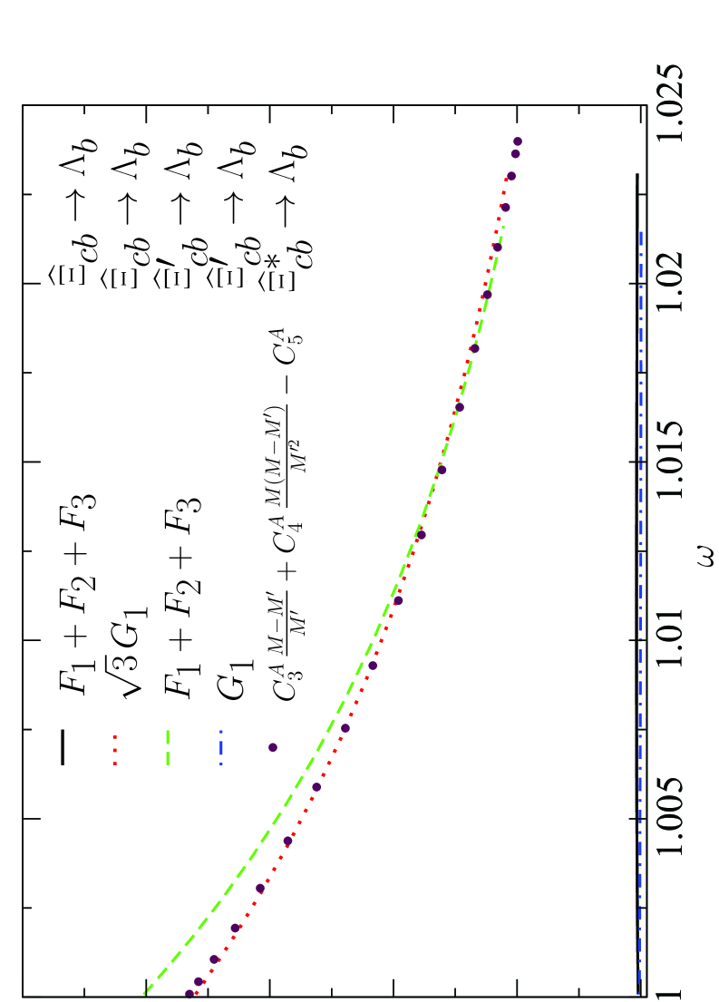
Figure 1: Test of HQSS constraints: Different combinations of form factors obtained in this work for several transitions with a $\Lambda_{b}$ in the final state ($S^{\prime}_{\rm light}=0$). For the calculation we have taken the masses of the $\widehat{\Xi}_{cb},\widehat{\Xi}^{\prime}_{cb}$ to be the masses of the physical states $\Xi^{(1)}_{cb},\Xi^{(2)}_{cb}$. Similar results are obtained for the $\widehat{\Omega}_{cb},\widehat{\Omega}^{\prime}_{cb},\widehat{\Omega}^{*}_{cb}\to\Xi_{b}$ and the $\widehat{\Xi}_{cb},\widehat{\Xi}^{\prime}_{cb},\widehat{\Xi}^{*}_{cb}\to\Xi_{b}$ transitions.

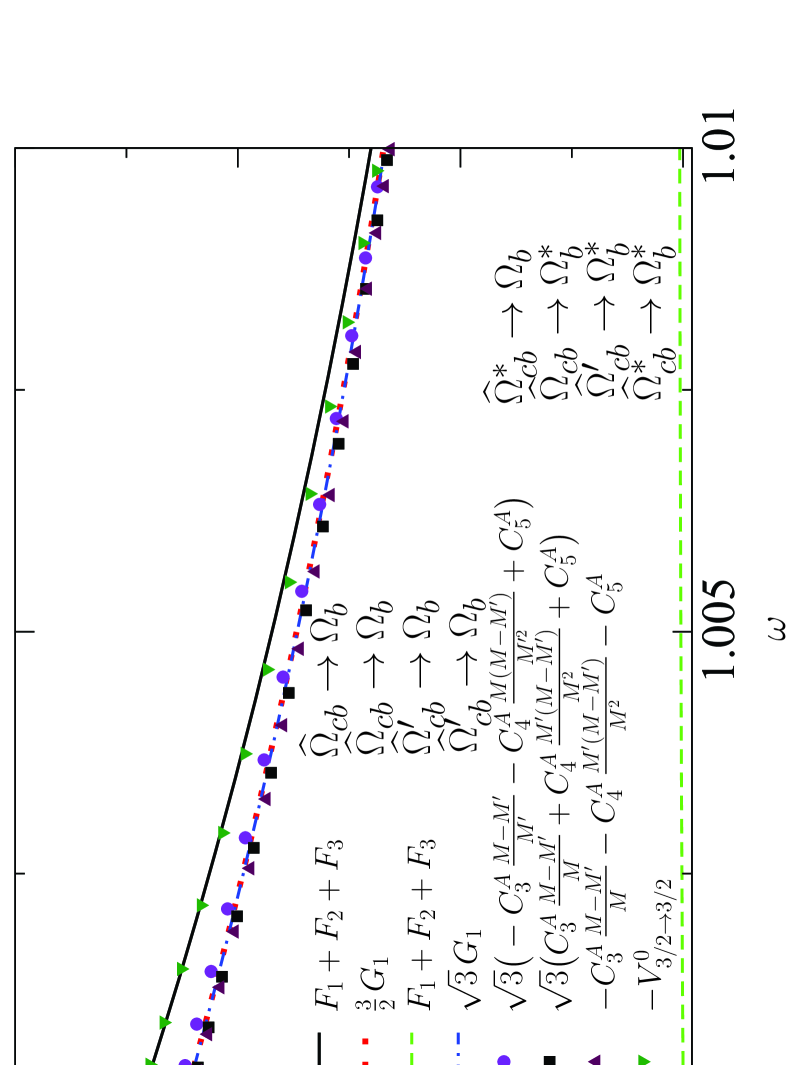
Figure 2: Test of HQSS constraints: Different combinations of form factors obtained in this work for transitions with a $\Omega_{b},\,\Omega^{*}_{b}$ in the final state ($S^{\prime}_{\rm light}=1$). $V^{0}_{3/2\to 3/2}$ stands for the matrix element of the zero component of the vector current for spin projections 3/2 both in the initial and final baryon. For the calculation we have taken the masses of the $\widehat{\Omega}_{cb},\widehat{\Omega}^{\prime}_{cb}$ to be the masses of the physical states $\Omega^{(1)}_{cb},\Omega^{(2)}_{cb}$. Similar results are obtained for the $\widehat{\Xi}_{cb},\widehat{\Xi}^{\prime}_{cb},\widehat{\Xi}^{*}_{cb}\to\Sigma_{b},\Sigma^{*}_{b}$, the $\widehat{\Xi}_{cb},\widehat{\Xi}^{\prime}_{cb},\widehat{\Xi}^{*}_{cb}\to\Xi^{\prime}_{b},\Xi^{*}_{b}$, and the $\widehat{\Omega}_{cb},\widehat{\Omega}^{\prime}_{cb},\widehat{\Omega}^{*}_{cb}\to\Xi^{\prime}_{b},\Xi^{*}_{b}$ transitions.

The results of Figs. 1 and 2 show HQSS is then a useful tool to understand the dynamics of the $c\to s,d$ decays of $cb$ baryons, as it was also the case for their CKM suppressed $b\to c$ decays Hernandez:2007qv ; Albertus:2009ww . We take advantage of this fact and we now use the HQSS approximate hadronic amplitudes in Eqs. (29), (31), (33), (35), (37), (39), (41), (43) and (45) to obtain model independent, though approximate, relations between different decay widths. With the use of those HQSS amplitudes and the leptonic tensor in Eq.(12) we obtain that near zero recoil

$$\widehat{B}_{cb}\to\Lambda_{b},\Xi_{b}\hskip 28.45274pt{\cal L}^{\alpha\beta}H_{\alpha\beta} \approx \frac{2MM^{\prime}}{3}\eta^{2}\bigg{[}-A(4+2\omega)+B\bigg{(}2\frac{(v\cdot q)(v^{\prime}\cdot q)}{q^{2}}-(\omega+1)\bigg{)}\bigg{]},$$ (46)

$$\widehat{B}^{\prime}_{cb}\to\Lambda_{b},\Xi_{b}\hskip 28.45274pt{\cal L}^{\alpha\beta}H_{\alpha\beta} \approx {2MM^{\prime}\eta^{2}}\bigg{[}A(4-2\omega)+B\bigg{(}2\frac{(v\cdot q)(v^{\prime}\cdot q)}{q^{2}}-(\omega-1)\bigg{)}\bigg{]},$$ (47)

$$\widehat{B}^{*}_{cb}\to\Lambda_{b},\Xi_{b}\hskip 28.45274pt{\cal L}^{\alpha\beta}H_{\alpha\beta} \approx \frac{2MM^{\prime}}{3}\eta^{2}(\omega+1)\bigg{[}-3A+B\bigg{(}\frac{(v^{\prime}\cdot q)^{2}}{q^{2}}-1\bigg{)}\bigg{]},$$ (48)

$$\widehat{B}_{cb}\to\Sigma_{b},\Xi^{\prime}_{b},\Omega_{b}\hskip 28.45274pt{\cal L}^{\alpha\beta}H_{\alpha\beta} \approx 2MM^{\prime}\beta^{2}\bigg{[}A\frac{1}{9}(20-26\omega)+B\frac{1}{9}\bigg{(}26\frac{(v\cdot q)(v^{\prime}\cdot q)}{q^{2}}+(5-13\omega)\bigg{)}\bigg{]},$$ (49)

$$\widehat{B}^{\prime}_{cb}\to\Sigma_{b},\Xi^{\prime}_{b},\Omega_{b}\hskip 28.45274pt{\cal L}^{\alpha\beta}H_{\alpha\beta} \approx \frac{2MM^{\prime}}{3}\beta^{2}\bigg{[}-A(4+2\omega)+B\bigg{(}2\frac{(v\cdot q)(v^{\prime}\cdot q)}{q^{2}}-(\omega+1)\bigg{)}\bigg{]},$$ (50)

$$\widehat{B}^{*}_{cb}\to\Sigma_{b},\Xi^{\prime}_{b},\Omega_{b}\hskip 28.45274pt{\cal L}^{\alpha\beta}H_{\alpha\beta} \approx \frac{2MM^{\prime}}{9}\beta^{2}(\omega+1)\bigg{[}-3A+B\bigg{(}\frac{(v\cdot q)^{2}}{q^{2}}-1\bigg{)}\bigg{]},$$ (51)

$$\widehat{B}_{cb}\to\Sigma^{*}_{b},\Xi^{*}_{b},\Omega^{*}_{b}\hskip 28.45274pt{\cal L}^{\alpha\beta}H_{\alpha\beta} \approx \frac{4MM^{\prime}}{9}\beta^{2}(\omega+1)\bigg{[}-3A+B\bigg{(}\frac{(v^{\prime}\cdot q)^{2}}{q^{2}}-1\bigg{)}\bigg{]},$$ (52)

$$\widehat{B}^{\prime}_{cb}\to\Sigma^{*}_{b},\Xi^{*}_{b},\Omega^{*}_{b}\hskip 28.45274pt{\cal L}^{\alpha\beta}H_{\alpha\beta} \approx \frac{4MM^{\prime}}{3}\beta^{2}(\omega+1)\bigg{[}-3A+B\bigg{(}\frac{(v^{\prime}\cdot q)^{2}}{q^{2}}-1\bigg{)}\bigg{]},$$ (53)

$$\widehat{B}^{*}_{cb}\to\Sigma^{*}_{b},\Xi^{*}_{b},\Omega^{*}_{b}\hskip 28.45274pt{\cal L}^{\alpha\beta}H_{\alpha\beta} \approx MM^{\prime}\beta^{2}\bigg{[}-A\frac{8}{9}\omega\big{(}1+2\omega^{2}\big{)}+B\frac{2}{9}\bigg{(}\frac{(v\cdot q)(v^{\prime}\cdot q)}{q^{2}}(20+8\omega^{2})-\omega\big{(}6+4\omega^{2}\big{)}\bigg{)}\bigg{]}.$$

We can now follow our work in Ref Hernandez:2007qv and, near zero recoil, take $\omega\approx 1$ and, because $v^{\prime}\approx v$, also approximate

$$\frac{(v\cdot q)^{2}}{q^{2}}\approx\frac{(v^{\prime}\cdot q)(v\cdot q)}{q^{2}}\approx\frac{(v^{\prime}\cdot q)^{2}}{q^{2}}.$$ (55)

Besides, for a light lepton $e$ or $\mu$ we have that $B\approx-A$ near zero recoil.

Using those approximations and denoting by $X$ the quantity in Eq.(55) we arrive at the following approximate results valid near zero recoil

$$\widehat{B}_{cb}\to\Lambda_{b},\Xi_{b}\hskip 28.45274pt{\cal L}^{\alpha\beta}H_{\alpha\beta} \approx -\frac{4MM^{\prime}}{3}\eta^{2}A\big{(}2+X\big{)},$$ (56)

$$\widehat{B}^{\prime}_{cb}\to\Lambda_{b},\Xi_{b}\hskip 28.45274pt{\cal L}^{\alpha\beta}H_{\alpha\beta} \approx {4MM^{\prime}\eta^{2}}A\big{(}1-X\big{)},$$ (57)

$$\widehat{B}^{*}_{cb}\to\Lambda_{b},\Xi_{b}\hskip 28.45274pt{\cal L}^{\alpha\beta}H_{\alpha\beta} \approx -\frac{4MM^{\prime}}{3}\eta^{2}A\big{(}2+X\big{)},$$ (58)

$$\widehat{B}_{cb}\to\Sigma_{b},\Xi^{\prime}_{b},\Omega_{b}\hskip 28.45274pt{\cal L}^{\alpha\beta}H_{\alpha\beta} \approx \frac{4MM^{\prime}}{9}\beta^{2}A\big{(}1-13X\big{)},$$ (59)

$$\widehat{B}^{\prime}_{cb}\to\Sigma_{b},\Xi^{\prime}_{b},\Omega_{b}\hskip 28.45274pt{\cal L}^{\alpha\beta}H_{\alpha\beta} \approx -\frac{4MM^{\prime}}{3}\beta^{2}A\big{(}2+X\big{)},$$ (60)

$$\widehat{B}^{*}_{cb}\to\Sigma_{b},\Xi^{\prime}_{b},\Omega_{b}\hskip 28.45274pt{\cal L}^{\alpha\beta}H_{\alpha\beta} \approx -\frac{4MM^{\prime}}{9}\beta^{2}A\big{(}2+X\big{)},$$ (61)

$$\widehat{B}_{cb}\to\Sigma^{*}_{b},\Xi^{*}_{b},\Omega^{*}_{b}\hskip 28.45274pt{\cal L}^{\alpha\beta}H_{\alpha\beta} \approx -\frac{8MM^{\prime}}{9}\beta^{2}A\big{(}2+X\big{)},$$ (62)

$$\widehat{B}^{\prime}_{cb}\to\Sigma^{*}_{b},\Xi^{*}_{b},\Omega^{*}_{b}\hskip 28.45274pt{\cal L}^{\alpha\beta}H_{\alpha\beta} \approx -\frac{8MM^{\prime}}{3}\beta^{2}A\big{(}2+X\big{)},$$ (63)

$$\widehat{B}^{*}_{cb}\to\Sigma^{*}_{b},\Xi^{*}_{b},\Omega^{*}_{b}\hskip 28.45274pt{\cal L}^{\alpha\beta}H_{\alpha\beta} \approx -\frac{4MM^{\prime}}{9}\beta^{2}A\big{(}1+14X\big{)}.$$ (64)

Can one extrapolate the above expressions over the whole $\omega$ range available in a given transition? In fact $B\approx-A$ to a very high degree (better than one percent) practically in the whole $\omega$ range accessible in these decays. On the other hand one has that $v\cdot q=M-M^{\prime}\omega$, $v^{\prime}\cdot q=M\omega-M^{\prime}$ and one expects larger deviations in approximate relation in Eq. (55) for $\omega\approx\omega_{\rm max}$. For instance for the $\widehat{\Xi}_{cb}\to\Lambda_{b}$ transition, one finds that $\frac{v^{\prime}\cdot q}{v\cdot q}=1.20$ for $\omega=1+0.9(\omega_{\rm max}-1)$. Fortunately, the differential decay distributions peak at much smaller $\omega$ values, so that errors related to the use of Eq. (55) in the whole $\omega$ range are less relevant. We show this in Figs. 3 and 4, where we give differential decay widths for transitions with a $\Lambda_{b}$ or an $\Omega^{(*)}_{b}$ in its final state. We have assumed the masses of the $\widehat{B}_{cb},\widehat{B}^{\prime}_{cb}$ to be the masses of the physical states $B^{(1)}_{cb},B^{(2)}_{cb}$.

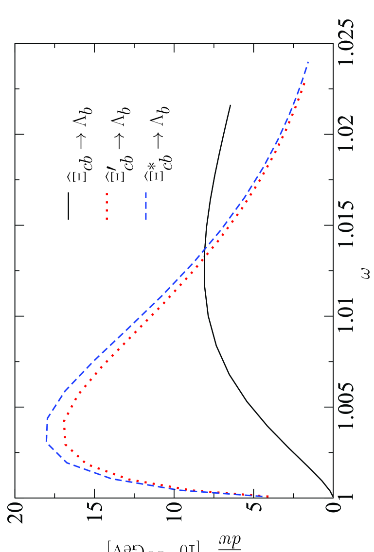
Figure 3: Differential decay widths for the specified transitions.

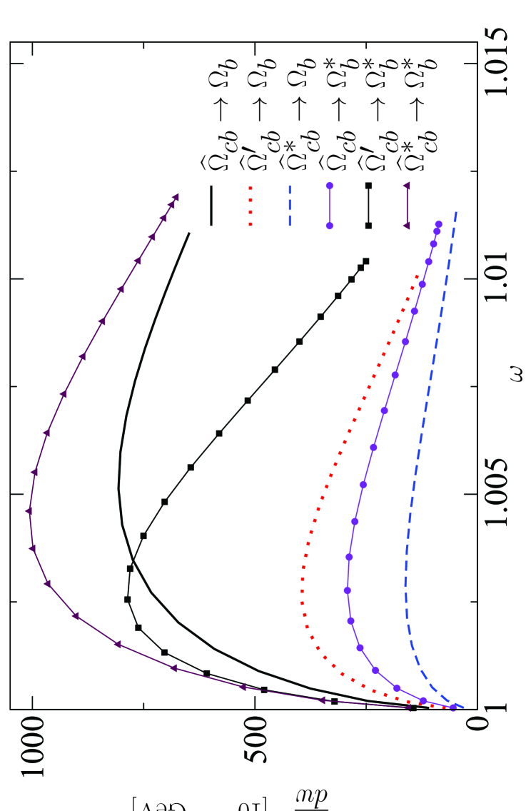
Figure 4: Differential decay widths for the specified transitions.

With this in mind and further assuming $M_{B_{cb}}=M_{B^{\prime}_{cb}}=M_{B^{*}_{cb}}$ and $M_{B_{b}}=M_{B^{\prime}_{b}}=M_{B^{*}_{b}}$ we can make the following approximate predictions based on HQSS

$$\Gamma(\widehat{\Xi}_{cb}\to\Lambda_{b}) \approx \Gamma(\widehat{\Xi}^{*}_{cb}\to\Lambda_{b}),$$

$$\Gamma(\widehat{B}_{cb}\to\Xi_{b}) \approx \Gamma(\widehat{B}^{*}_{cb}\to\Xi_{b}),$$ (65)

$$\Gamma(\widehat{\Xi}^{\prime}_{cb}\to\Sigma_{b}) \approx 3\Gamma(\widehat{\Xi}^{*}_{cb}\to\Sigma_{b})\approx\frac{3}{2}\Gamma(\widehat{\Xi}_{cb}\to\Sigma^{*}_{b})\approx\frac{1}{2}\Gamma(\widehat{\Xi}^{\prime}_{cb}\to\Sigma^{*}_{b}),$$

$$\Gamma(\widehat{B}^{\prime}_{cb}\to\Xi^{\prime}_{b}) \approx 3\Gamma(\widehat{B}^{*}_{cb}\to\Xi^{\prime}_{b})\approx\frac{3}{2}\Gamma(\widehat{B}_{cb}\to\Xi^{*}_{b})\approx\frac{1}{2}\Gamma(\widehat{B}^{\prime}_{cb}\to\Xi^{*}_{b}),$$

$$\Gamma(\widehat{\Omega}^{\prime}_{cb}\to\Omega_{b}) \approx 3\Gamma(\widehat{\Omega}^{*}_{cb}\to\Omega_{b})\approx\frac{3}{2}\Gamma(\widehat{\Omega}_{cb}\to\widehat{\Omega}^{*}_{b})\approx\frac{1}{2}\Gamma(\widehat{\Omega}^{\prime}_{cb}\to\Omega^{*}_{b}),$$ (66)

$$\Gamma(\widehat{\Xi}^{*}_{cb}\to\Sigma^{*}_{b}) \approx \Gamma(\widehat{\Xi}^{*}_{cb}\to\Sigma_{b})+\Gamma(\Xi_{cb}\to\Sigma_{b}),$$

$$\Gamma(\widehat{B}^{*}_{cb}\to\Xi^{*}_{b}) \approx \Gamma(\widehat{B}^{*}_{cb}\to\Xi^{\prime}_{b})+\Gamma(B_{cb}\to\Xi^{\prime}_{b}),$$

$$\Gamma(\widehat{\Omega}^{*}_{cb}\to\Omega^{*}_{b}) \approx \Gamma(\widehat{\Omega}^{*}_{cb}\to\Omega_{b})+\Gamma(\widehat{\Omega}_{cb}\to\Omega_{b}).$$ (67)

Assuming that the states $\widehat{B}_{cb},\widehat{B}^{\prime}_{cb}$ have the same masses as the physical states $B^{(1)}_{cb},B^{(2)}_{cb}$ we get the following numerical results (we give $\widetilde{\Gamma}=\frac{\Gamma}{10^{-14}\,{\rm GeV}}$)

$$\widetilde{\Gamma}(\widehat{\Xi}^{+}_{cb}\to\Lambda_{b}^{0}) \approx \widetilde{\Gamma}(\widehat{\Xi}^{*\,+}_{cb}\to\Lambda_{b}^{0})$$

$$0.219 \approx 0.235,$$ (68)

$$\widetilde{\Gamma}(\widehat{\Omega}^{0}_{cb}\to\Xi^{-}_{b}) \approx \widetilde{\Gamma}(\widehat{\Omega}^{*\,0}_{cb}\to\Xi^{-}_{b})$$

$$0.179 \approx 0.196,$$ (69)

$$\widetilde{\Gamma}(\widehat{\Xi}^{\,+}_{cb}\to\Xi^{0}_{b}) \approx \widetilde{\Gamma}(\widehat{\Xi}^{*\,+}_{cb}\to\Xi^{0}_{b})$$

$$3.74 \approx 4.08,$$ (70)

$$\widetilde{\Gamma}(\widehat{\Xi}^{\prime\,+}_{cb}\to\Sigma_{b}^{0})\approx 3\widetilde{\Gamma}(\widehat{\Xi}^{*\,+}_{cb}\to\Sigma_{b}^{0}) \approx \frac{3}{2}\widetilde{\Gamma}(\widehat{\Xi}^{+}_{cb}\to\Sigma^{*\,0}_{b})\approx\frac{1}{2}\widetilde{\Gamma}(\widehat{\Xi}^{\prime\,+}_{cb}\to\Sigma^{*\,0}_{b})$$

$$0.0930\approx 0.120 \approx 0.0946\approx 0.0813,$$ (71)

$$\widetilde{\Gamma}(\widehat{\Omega}^{\prime\,0}_{cb}\to\Xi^{\prime\,-}_{b})\approx 3\widetilde{\Gamma}(\widehat{\Omega}^{*\,0}_{cb}\to\Xi^{\prime\,-}_{b}) \approx \frac{3}{2}\widetilde{\Gamma}(\widehat{\Omega}^{0}_{cb}\to\Xi^{*\,-}_{b})\approx\frac{1}{2}\widetilde{\Gamma}(\widehat{\Omega}^{\prime\,0}_{cb}\to\Xi^{*\,-}_{b})$$

$$0.0776\approx 0.101 \approx 0.0826\approx 0.0714,$$ (72)

$$\widetilde{\Gamma}(\widehat{\Xi}^{\prime\,+}_{cb}\to\Xi_{b}^{\prime\,0})\approx 3\widetilde{\Gamma}(\widehat{\Xi}^{*\,+}_{cb}\to\Xi_{b}^{\prime\,0}) \approx \frac{3}{2}\widetilde{\Gamma}(\widehat{\Xi}^{+}_{cb}\to\Xi^{*\,0}_{b})\approx\frac{1}{2}\widetilde{\Gamma}(\widehat{\Xi}^{\prime\,+}_{cb}\to\Xi^{*\,0}_{b})$$

$$1.65\approx 2.24 \approx 1.74\approx 1.47,$$ (73)

$$\widetilde{\Gamma}(\widehat{\Omega}^{\prime\,0}_{cb}\to\Omega^{-}_{b})\approx 3\widetilde{\Gamma}(\widehat{\Omega}^{*\,0}_{cb}\to\Omega^{-}_{b}) \approx \frac{3}{2}\widetilde{\Gamma}(\widehat{\Omega}^{0}_{cb}\to\Omega^{*\,-}_{b})\approx\frac{1}{2}\widetilde{\Gamma}(\widehat{\Omega}^{\prime\,0}_{cb}\to\Omega^{*\,-}_{b})$$

$$2.98\approx 4.05 \approx 3.57\approx 3.01,$$ (74)

$$\widetilde{\Gamma}(\widehat{\Xi}^{*\,+}_{cb}\to\Sigma^{*\,0}_{b}) \approx \widetilde{\Gamma}(\widehat{\Xi}^{*\,+}_{cb}\to\Sigma_{b}^{0})+\widetilde{\Gamma}(\widehat{\Xi}_{cb}^{+}\to\Sigma_{b}^{0})$$

$$0.246 \approx 0.258,$$ (75)

$$\widetilde{\Gamma}(\widehat{\Omega}^{*\,0}_{cb}\to\Xi^{*\,-}_{b}) \approx \widetilde{\Gamma}(\widehat{\Omega}^{*\,0}_{cb}\to\Xi^{\prime-}_{b})+\widetilde{\Gamma}(\widehat{\Omega}^{0}_{cb}\to\Xi^{\prime-}_{b})$$

$$0.223 \approx 0.213,$$ (76)

$$\widetilde{\Gamma}(\widehat{\Xi}^{*\,+}_{cb}\to\Xi^{*\,0}_{b}) \approx \widetilde{\Gamma}(\widehat{\Xi}^{*\,+}_{csb}\to\Xi^{\prime 0}_{b})+\widetilde{\Gamma}(\widehat{\Xi}^{+}_{cb}\to\Xi^{\prime 0}_{b})$$

$$5.03 \approx 4.99,$$ (77)

$$\widetilde{\Gamma}(\widehat{\Omega}^{*\,0}_{cb}\to\Omega^{*\,-}_{b}) \approx \widetilde{\Gamma}(\widehat{\Omega}^{*\,0}_{cb}\to\Omega^{-}_{b})+\widetilde{\Gamma}(\widehat{\Omega}^{0}_{cb}\to\Omega^{-}_{b})$$

$$10.2 \approx 9.16.$$ (78)

We find our results agree in most of the cases at the level of 10% with some notable exceptions in Eqs. (71), (72), (73) and (74). These latter discrepancies are largely due, not to the the use of the approximate HQSS inspired relations in Eqs.(56) -(64), but to the fact that the different baryons that appear in the relations do not have the same mass, and therefore the available phase space is different for each transition. For instance if we just make the masses of ${\widehat{\Xi}^{*}_{cb}},{\widehat{\Xi}_{cb}}$ equal to the ${\widehat{\Xi}^{\prime}_{cb}}$ mass and the mass of $\Xi^{*}_{b}$ equal to the $\Xi^{\prime}_{b}$ mass we get

$$\widetilde{\Gamma}(\Xi^{\prime\,+}_{cb}\to\Xi_{b}^{\prime\,0})\approx 3\widetilde{\Gamma}(\Xi^{*\,+}_{cb}\to\Xi_{b}^{\prime\,0}) \approx \frac{3}{2}\widetilde{\Gamma}(\Xi^{+}_{cb}\to\Xi^{*\,0}_{b})\approx\frac{1}{2}\widetilde{\Gamma}(\Xi^{\prime\,+}_{cb}\to\Xi^{*\,0}_{b})$$

$$1.65\approx 1.69 \approx 1.66\approx 1.65,$$ (79)

or in the $\Omega$ sector, with similar changes in the masses,

$$\widetilde{\Gamma}(\Omega^{\prime\,+}_{cb}\to\Omega_{b}^{\prime\,0})\approx 3\widetilde{\Gamma}(\Omega^{*\,+}_{cb}\to\Omega_{b}^{\prime\,0}) \approx \frac{3}{2}\widetilde{\Gamma}(\Omega^{+}_{cb}\to\Omega^{*\,0}_{b})\approx\frac{1}{2}\widetilde{\Gamma}(\Omega^{\prime\,+}_{cb}\to\Omega^{*\,0}_{b})$$

$$2.98\approx 3.07 \approx 2.93\approx 2.91.$$ (80)

The agreement improves considerably. Then, the HQSS derived relations are appropriate to evaluate the hadronic amplitudes but the final results may be very sensitive on actual mass values.

Thus, mass differences and the variations induced by them in the available phase space can not be neglected. Besides the physical states $B^{(1)}_{cb},B^{(2)}_{cb}$ are not exactly equal to the $\widehat{B}_{cb},\widehat{B}^{\prime}_{cb}$ states and this could also affect some of the decay widths. In what follows we give the corresponding numbers for the physical states.

$$\widetilde{\Gamma}(\Xi^{(1)\,+}_{cb}\to\Lambda_{b}^{0}) \approx \widetilde{\Gamma}(\Xi^{*\,+}_{cb}\to\Lambda_{b}^{0})$$

$$0.219 \approx 0.235,$$ (81)

$$\widetilde{\Gamma}(\Omega^{(1)\,0}_{cb}\to\Xi^{-}_{b}) \approx \widetilde{\Gamma}(\Omega^{*\,0}_{cb}\to\Xi^{-}_{b})$$

$$0.179 \approx 0.196,$$ (82)

$$\widetilde{\Gamma}(\Xi^{(1)\,+}_{cb}\to\Xi^{0}_{b}) \approx \widetilde{\Gamma}(\Xi^{*\,+}_{cb}\to\Xi^{0}_{b})$$

$$3.73 \approx 4.08,$$ (83)

$$\widetilde{\Gamma}(\Xi^{(2)\,+}_{cb}\to\Sigma_{b}^{0})\approx 3\widetilde{\Gamma}(\Xi^{*\,+}_{cb}\to\Sigma_{b}^{0}) \approx \frac{3}{2}\widetilde{\Gamma}(\Xi^{(1)\,+}_{cb}\to\Sigma^{*\,0}_{b})\approx\frac{1}{2}\widetilde{\Gamma}(\Xi^{(2)\,+}_{cb}\to\Sigma^{*\,0}_{b})$$

$$0.110\approx 0.120 \approx 0.121\approx 0.0737,$$ (84)

$$\widetilde{\Gamma}(\Omega^{(2)\,0}_{cb}\to\Xi^{\prime\,-}_{b})\approx 3\widetilde{\Gamma}(\Omega^{*\,0}_{cb}\to\Xi^{\prime\,-}_{b}) \approx \frac{3}{2}\widetilde{\Gamma}(\Omega^{(1)\,0}_{cb}\to\Xi^{*\,-}_{b})\approx\frac{1}{2}\widetilde{\Gamma}(\Omega^{(2)\,0}_{cb}\to\Xi^{*\,-}_{b})$$

$$0.0907\approx 0.101 \approx 0.104\approx 0.0652,$$ (85)

$$\widetilde{\Gamma}(\Xi^{(2)\,+}_{cb}\to\Xi_{b}^{\prime\,0})\approx 3\widetilde{\Gamma}(\Xi^{*\,+}_{cb}\to\Xi_{b}^{\prime\,0}) \approx \frac{3}{2}\widetilde{\Gamma}(\Xi^{(1)\,+}_{cb}\to\Xi^{*\,0}_{b})\approx\frac{1}{2}\widetilde{\Gamma}(\Xi^{(2)\,+}_{cb}\to\Xi^{*\,0}_{b})$$

$$1.95\approx 2.24 \approx 2.29\approx 1.34,$$ (86)

$$\widetilde{\Gamma}(\Omega^{(2)\,0}_{cb}\to\Omega^{-}_{b})\approx 3\widetilde{\Gamma}(\Omega^{*\,0}_{cb}\to\Omega^{-}_{b}) \approx \frac{3}{2}\widetilde{\Gamma}(\Omega^{(1)\,0}_{cb}\to\Omega^{*\,-}_{b})\approx\frac{1}{2}\widetilde{\Gamma}(\Omega^{(2)\,0}_{cb}\to\Omega^{*\,-}_{b})$$

$$3.49\approx 4.05 \approx 4.48\approx 2.75,$$ (87)

$$\widetilde{\Gamma}(\Xi^{*\,+}_{cb}\to\Sigma^{*\,0}_{b}) \approx \widetilde{\Gamma}(\Xi^{*\,+}_{cb}\to\Sigma_{b}^{0})+\widetilde{\Gamma}(\Xi_{cb}^{(1)\,+}\to\Sigma_{b}^{0})$$

$$0.246 \approx 0.238,$$ (88)

$$\widetilde{\Gamma}(\Omega^{*\,0}_{cb}\to\Xi^{*\,-}_{b}) \approx \widetilde{\Gamma}(\Omega^{*\,0}_{cb}\to\Xi^{\prime-}_{b})+\widetilde{\Gamma}(\Omega^{(1)\,0}_{cb}\to\Xi^{\prime-}_{b})$$

$$0.223 \approx 0.203,$$ (89)

$$\widetilde{\Gamma}(\Xi^{*\,+}_{cb}\to\Xi^{*\,0}_{b}) \approx \widetilde{\Gamma}(\Xi^{*\,+}_{csb}\to\Xi^{\prime 0}_{b})+\widetilde{\Gamma}(\Xi^{(1)\,+}_{cb}\to\Xi^{\prime 0}_{b})$$

$$5.03 \approx 4.62$$ (90)

$$\widetilde{\Gamma}(\Omega^{*\,0}_{cb}\to\Omega^{*\,-}_{b}) \approx \widetilde{\Gamma}(\Omega^{*\,0}_{cb}\to\Omega^{-}_{b})+\widetilde{\Gamma}(\Omega^{(1)\,0}_{cb}\to\Omega^{-}_{b})$$

$$10.2 \approx 8.56.$$ (91)

Most of the relations are satisfied at the 10% level with a few notable exceptions that involve the decay widths for the $\Xi^{(2)}_{cb}\to\Sigma^{*}_{b},\,\Xi^{*}_{b}$ and $\Omega^{(2)\,0}_{cb}\to\Xi^{*\,-}_{b},\,\Omega^{*\,-}_{b}$ transitions.

V Summary

We have made a systematic study of semileptonic decays of $cb$ ground-state doubly heavy baryons driven by $c\to s,d$ transitions at the quark level. We have employed a simple constituent quark model scheme, which benefits from the important simplifications in the solution of the non-relativistic three body problem that stem from the application of HQSS Albertus:2003sx ; Albertus:2006wb . Despite the modulus of CKM matrix elements $|V_{cs}|,\,|V_{cd}|$ are much larger than $|V_{cb}|$, the smaller available phase space leads to $c\to s$ decay widths that turn out to be larger but of the same order of magnitude as the $b\to c$ driven processes, while widths for $c\to d$ transitions are much smaller.

As for $b\to c$ semileptonic pervin2 ; Albertus:2009ww and electromagnetic Albertus:2010hi ; Branz:2010pq decays, here also hyperfine mixing effects have a tremendous impact on $c\to s,d$ semileptonic decays of spin-1/2 $cb$ baryons. We find factors of 2 corrections in many cases due to mixing.

We have derived for the first time HQSS relations for the hadronic amplitudes. By requiring invariance under separate bottom and charm quark spin rotations, we have obtained constraints on the form factors that enormously simplify the description of these decays. Though, these relations are strictly valid in the limit of very large heavy quark masses and near zero recoil, they turn out to be reasonable accurate for the whole available phase space in these decays. Indeed, we find our calculation is consistent with HQSS and only deviations at the 10% level are observed due to the actual, finite, heavy quark masses. With the use of the HQSS relations and assuming $M_{B_{cb}}=M_{B^{\prime}_{cb}}=M_{B^{*}_{cb}}$ and $M_{B_{b}}=M_{B^{\prime}_{b}}=M_{B^{*}_{b}}$, we have made model independent, though approximate, predictions for ratios of decay widths. Our values for those ratios agree with the HQSS motivated predictions at the level of 10% in most of the cases. We expect those predictions to hold to that level of accuracy in other approaches.

Appendix A Nonrelativistic baryon states and wave functions

We construct our nonrelativistic states as follows

$$\big{|}{B,r\,\vec{P}}\,\big{\rangle}_{NR}=\sqrt{2E}\int d^{\,3}Q_{1}\int d^{\,3}Q_{2}\ {\cal S}_{B}\sum_{\alpha_{1},\alpha_{2},\alpha_{3}}\widehat{\psi}^{(B,r)}_{\alpha 1\,\alpha_{2}\,\alpha_{3}}(\,\vec{Q}_{1},\vec{Q}_{2}\,)\ \frac{1}{(2\pi)^{3}\ \sqrt{2E_{f_{1}}2E_{f_{2}}2E_{f_{3}}}}$$

$$\hskip 85.35826pt\times\big{|}\ \alpha_{1}\ \vec{p}_{1}=\frac{m_{f_{1}}}{\overline{M}}\vec{P}+\vec{Q}_{1}\ \big{\rangle}\big{|}\ \alpha_{2}\ \vec{p}_{2}=\frac{m_{f_{2}}}{\overline{M}}\vec{P}+\vec{Q}_{2}\ \big{\rangle}\big{|}\ \alpha_{3}\ \vec{p}_{3}=\frac{m_{f_{3}}}{\overline{M}}\vec{P}-\vec{Q}_{1}-\vec{Q}_{2}\ \big{\rangle}.$$ (92)

The factor $\sqrt{2E}$ is introduced for convenience in order to have the proper normalization. We denote by $\alpha_{j}$ the spin ($s$), flavor ($f$) and color ($c$) quantum numbers ( $\alpha\equiv(s,f,c)$ ) of the $j-$th quark with $(E_{f_{j}},\,\vec{p}_{j})$ and $m_{f_{j}}$ its four-momentum and mass, and $\overline{M}=m_{f_{1}}+m_{f_{2}}+m_{f_{3}}$. Individual quark states are normalized such that $\left\langle\ \alpha^{\prime}\ \vec{p}^{\ \prime}\,|\,\alpha\ \vec{p}\,\right\rangle=2E_{f}\,(2\pi)^{3}\,\delta_{\alpha^{\prime}\,\alpha}\,\delta^{3}(\vec{p}^{\ \prime}-\vec{p}\,)$. $\widehat{\psi}^{\,(B,r)}_{\alpha_{1}\,\alpha_{2}\,\alpha_{3}}(\,\vec{Q}_{1},\vec{Q}_{2}\,)$ is the internal wave function in momentum space, being $\vec{Q}_{1}$ ($\vec{Q}_{2}$) the conjugate momenta to the relative position $\vec{r}_{1}$ ($\vec{r}_{2}$) between quark 1 (2) and the third quark. In the transitions under study an initial $c\,b\,l^{\prime}$ baryon decays into a final $l\,l^{\prime}\,b$ one, where $l=d,s$ and $l^{\prime}=u,d,s$. We construct the wave functions such that the $c$ and $b$ quarks in the initial baryon are quarks 1 and 2 respectively. Also in the final baryon the two light quarks $l$ and $l^{\prime}$ are respectively quarks 1 and 2. Expressions for the different $\widehat{\psi}^{(B,r)}_{\alpha_{1}\,\alpha_{2}\,\alpha_{3}}(\,\vec{Q}_{1},\vec{Q}_{2}\,)$ are given below. These wave functions are normalized as

$$\int d^{\,3}Q_{1}\int d^{\,3}Q_{2}\ \sum_{\alpha_{1},\alpha_{2},\alpha_{3}}\left(\widehat{\psi}^{(B,r^{\prime})}_{\alpha_{1}\,\alpha_{2}\,\alpha_{3}}(\,\vec{Q}_{1},\vec{Q}_{2}\,)\right)^{*}\widehat{\psi}^{(B,r)}_{\alpha_{1}\,\alpha_{2}\,\alpha_{3}}(\,\vec{Q}_{1},\vec{Q}_{2}\,)=\delta_{rr^{\prime}}.$$ (93)

For the final states we use wave functions that are antisymmetric under the exchange of quarks 1 and 2 quantum numbers. In order for our nonrelativistic baryon states to have the proper normalization

$${}_{\stackrel{{\scriptstyle}}{{NR}}}\big{\langle}\,{B,r^{\prime}\,\vec{P}^{\,\prime}}\,|\,{B,r\,\vec{P}}\,\big{\rangle}_{NR}=2E\,(2\pi)^{3}\,\delta_{rr^{\prime}}\,\delta^{3}(\vec{P}^{\,\prime}-\vec{P}\,).$$ (94)

we need to introduce in Eq. (A) a symmetry factor ${\cal S}_{B}=\frac{1}{\sqrt{2}}$ for those states. For the initial states ${\cal S}_{B}=1$.

The wave functions for $cb$ states where the spin of the heavy quark subsystem is well defined are given by

$$\widehat{\psi}^{\,(\Xi^{+}_{cb},s)}_{\alpha_{1}\,\alpha_{2}\,\alpha_{3}}(\,\vec{Q}_{1},\vec{Q}_{2}\,) = \frac{1}{\sqrt{3!}}\,\varepsilon_{c_{1}\,c_{2}\,c_{3}}\ \widehat{\phi}^{\,(\Xi^{+}_{cb},s)}_{(s_{1},\,f_{1})\ ,(s_{2},\,f_{2})\,(s_{3},\,f_{3})}(\,\vec{Q}_{1},\vec{Q}_{2}\,)$$ (95)

$$= \frac{1}{\sqrt{3!}}\,\varepsilon_{c_{1}\,c_{2}\,c_{3}}\ \ \widetilde{\phi}^{\,(\Xi_{cb})}(\,\vec{Q}_{1},\vec{Q}_{2}\,)\ \delta_{f_{1}\,c}\,\delta_{f_{2}\,b}\,\delta_{f_{3}\,u}$$

$$\hskip 56.9055pt\times\ (1/2,1/2,1;s_{1},s_{2},s_{1}+s_{2})\ (1,1/2,1/2;s_{1}+s_{2},s_{3},s),$$

$$\widehat{\psi}^{\,(\Xi^{{}^{\prime}+}_{cb},s)}_{\alpha_{1}\,\alpha_{2}\,\alpha_{3}}(\,\vec{Q}_{1},\vec{Q}_{2}\,) = \frac{1}{\sqrt{3!}}\,\varepsilon_{c_{1}\,c_{2}\,c_{3}}\ \widehat{\phi}^{\,(\Xi^{{}^{\prime}+}_{cb},s)}_{(s_{1},\,f_{1})\ ,(s_{2},\,f_{2})\,(s_{3},\,f_{3})}(\,\vec{Q}_{1},\vec{Q}_{2}\,)$$ (96)

$$= \frac{1}{\sqrt{3!}}\,\varepsilon_{c_{1}\,c_{2}\,c_{3}}\ \ \widetilde{\phi}^{\,(\Xi_{cb})}(\,\vec{Q}_{1},\vec{Q}_{2}\,)\ \delta_{f_{1}\,c}\,\delta_{f_{2}\,b}\,\delta_{f_{3}\,u}\ (1/2,1/2,0;s_{1},s_{2},0)\,\delta_{s_{3}\,s},$$

$$\widehat{\psi}^{\,(\Xi^{*+}_{cb},s)}_{\alpha_{1}\,\alpha_{2}\,\alpha_{3}}(\,\vec{Q}_{1},\vec{Q}_{2}\,) = \frac{1}{\sqrt{3!}}\,\varepsilon_{c_{1}\,c_{2}\,c_{3}}\ \widehat{\phi}^{\,(\Xi^{*+}_{cb},s)}_{(s_{1},\,f_{1})\ ,(s_{2},\,f_{2})\,(s_{3},\,f_{3})}(\,\vec{Q}_{1},\vec{Q}_{2}\,)$$ (97)

$$= \frac{1}{\sqrt{3!}}\,\varepsilon_{c_{1}\,c_{2}\,c_{3}}\ \ \widetilde{\phi}^{\,(\Xi^{*}_{cb})}(\,\vec{Q}_{1},\vec{Q}_{2}\,)\ \delta_{f_{1}\,c}\,\delta_{f_{2}\,b}\,\delta_{f_{3}\,u}$$

$$\hskip 56.9055pt\times\ (1/2,1/2,1;s_{1},s_{2},s_{1}+s_{2})\ (1,1/2,3/2;s_{1}+s_{2},s_{3},s),$$

where $\varepsilon_{c_{1}c_{2}c_{3}}$ is the totally antisymmetric tensor with $\frac{\varepsilon_{c_{1}c_{2}c_{3}}}{\sqrt{3!}}$ being the fully antisymmetric color wave function. The $(j_{1},j_{2},j;m_{1},m_{2},m)$ are SU(2) Clebsch-Gordan coefficients. The different $\tilde{\phi}(\,\vec{Q}_{1},\vec{Q}_{2}\,)$ wave functions have total orbital angular momentum 0 being invariant under rotations and thus depending only on $|\vec{Q}_{1}|$, $|\vec{Q}_{2}|$ and $\vec{Q}_{1}\cdot\vec{Q}_{2}$. They are normalized such that

$$\int d^{\,3}Q_{1}\int d^{\,3}Q_{2}\ \left|\widetilde{\phi}(\,\vec{Q}_{1},\vec{Q}_{2}\,)\right|^{2}=1.$$ (98)

The corresponding $\Xi^{(^{\prime}*)}$ neutral states are obtained by implementing the trivial replacement $\delta_{f_{3}\,u}\to\delta_{f_{3}\,d}$. Besides, the $\Omega^{(^{\prime}*)}$ color-spin-flavor-momentum wave-functions are obtained from the cascade ones by substituting the momentum space $\widetilde{\phi}^{\,\Xi^{(^{\prime}*)}_{cb}}(\,\vec{Q}_{1},\vec{Q}_{2}\,)$ wave functions by the appropriated $\widetilde{\phi}^{\,\Omega^{(^{\prime}*)}_{cb}}(\,\vec{Q}_{1},\vec{Q}_{2}\,)$ ones, and always using $\delta_{f_{3}\,s}$. For $b$-heavy baryons we further have

$$\widehat{\psi}^{\,(\Lambda^{0}_{b},s)}_{\alpha_{1}\,\alpha_{2}\,\alpha_{3}}(\,\vec{Q}_{1},\vec{Q}_{2}\,) = \frac{1}{\sqrt{3!}}\,\varepsilon_{c_{1}\,c_{2}\,c_{3}}\ \widehat{\phi}^{\,(\Lambda^{0}_{b},s)}_{(s_{1},\,f_{1})\ ,(s_{2},\,f_{2})\,(s_{3},\,f_{3})}(\,\vec{Q}_{1},\vec{Q}_{2}\,)$$ (99)

$$= \frac{1}{\sqrt{3!}}\,\varepsilon_{c_{1}\,c_{2}\,c_{3}}\ \ \widetilde{\phi}^{\,(\Lambda^{0}_{b})}(\,\vec{Q}_{1},\vec{Q}_{2}\,)\ \frac{1}{\sqrt{2}}(\delta_{f_{1}\,u}\,\delta_{f_{2}\,d}-\delta_{f_{1}\,d}\,\delta_{f_{2}\,u})\delta_{f_{3}\,b}(1/2,1/2,0;s_{1},s_{2},0)\,\delta_{s_{3}\,s},$$

$$\widehat{\psi}^{\,(\Sigma^{0}_{b},s)}_{\alpha_{1}\,\alpha_{2}\,\alpha_{3}}(\,\vec{Q}_{1},\vec{Q}_{2}\,) = \frac{1}{\sqrt{3!}}\,\varepsilon_{c_{1}\,c_{2}\,c_{3}}\ \widehat{\phi}^{\,(\Sigma^{0}_{b},s)}_{(s_{1},\,f_{1})\ ,(s_{2},\,f_{2})\,(s_{3},\,f_{3})}(\,\vec{Q}_{1},\vec{Q}_{2}\,)$$ (100)

$$= \frac{1}{\sqrt{3!}}\,\varepsilon_{c_{1}\,c_{2}\,c_{3}}\ \ \widetilde{\phi}^{\,(\Sigma_{b})}(\,\vec{Q}_{1},\vec{Q}_{2}\,)\ \frac{1}{\sqrt{2}}(\delta_{f_{1}\,u}\,\delta_{f_{2}\,d}+\delta_{f_{1}\,d}\,\delta_{f_{2}\,u})\delta_{f_{3}\,b}$$

$$\hskip 14.22636pt\times\,(1/2,1/2,1;s_{1},s_{2},s_{1}+s_{2})(1,1/2,1/2,s_{1}+s_{2},s_{3},s),$$

$$\widehat{\psi}^{\,(\Sigma^{*0}_{b},s)}_{\alpha_{1}\,\alpha_{2}\,\alpha_{3}}(\,\vec{Q}_{1},\vec{Q}_{2}\,) = \frac{1}{\sqrt{3!}}\,\varepsilon_{c_{1}\,c_{2}\,c_{3}}\ \widehat{\phi}^{\,(\Sigma^{*0}_{b},s)}_{(s_{1},\,f_{1})\ ,(s_{2},\,f_{2})\,(s_{3},\,f_{3})}(\,\vec{Q}_{1},\vec{Q}_{2}\,)$$ (101)

$$= \frac{1}{\sqrt{3!}}\,\varepsilon_{c_{1}\,c_{2}\,c_{3}}\ \ \widetilde{\phi}^{\,(\Sigma^{*}_{b})}(\,\vec{Q}_{1},\vec{Q}_{2}\,)\ \frac{1}{\sqrt{2}}(\delta_{f_{1}\,u}\,\delta_{f_{2}\,d}+\delta_{f_{1}\,d}\,\delta_{f_{2}\,u})\delta_{f_{3}\,b}$$

$$\hskip 14.22636pt\times\,(1/2,1/2,1;s_{1},s_{2},s_{1}+s_{2})(1,1/2,3/2,s_{1}+s_{2},s_{3},s),$$

$$\widehat{\psi}^{\,(\Xi^{0}_{b},s)}_{\alpha_{1}\,\alpha_{2}\,\alpha_{3}}(\,\vec{Q}_{1},\vec{Q}_{2}\,) = \frac{1}{\sqrt{3!}}\,\varepsilon_{c_{1}\,c_{2}\,c_{3}}\ \widehat{\phi}^{\,(\Xi^{0}_{b},s)}_{(s_{1},\,f_{1})\,(s_{2},\,f_{2})\,(s_{3},\,f_{3})}(\,\vec{Q}_{1},\vec{Q}_{2}\,)$$ (102)

$$= \frac{1}{\sqrt{3!}}\,\varepsilon_{c_{1}\,c_{2}\,c_{3}}\ \ \frac{1}{\sqrt{2}}\,(\widetilde{\phi}^{\,(\Xi^{0}_{b})}_{us}(\,\vec{Q}_{1},\vec{Q}_{2}\,)\ \delta_{f_{1}\,u}\,\delta_{f_{2}\,s}-\widetilde{\phi}^{\,(\Xi^{0}_{b})}_{su}(\,\vec{Q}_{1},\vec{Q}_{2}\,)\ \delta_{f_{1}\,s}\,\delta_{f_{2}\,u})\,\delta_{f_{3}\,b}$$

$$\hskip 56.9055pt\times\ (1/2,1/2,0;s_{1},s_{2},0)\,\delta_{s_{3}\,s},$$

$$\widehat{\psi}^{\,(\Xi^{\prime\,0}_{b},s)}_{\alpha_{1}\,\alpha_{2}\,\alpha_{3}}(\,\vec{Q}_{1},\vec{Q}_{2}\,) = \frac{1}{\sqrt{3!}}\,\varepsilon_{c_{1}\,c_{2}\,c_{3}}\ \widehat{\phi}^{\,(\Xi^{\prime\,0}_{b},s)}_{(s_{1},\,f_{1})\,(s_{2},\,f_{2})\,(s_{3},\,f_{3})}(\,\vec{Q}_{1},\vec{Q}_{2}\,)$$ (103)

$$= \frac{1}{\sqrt{3!}}\,\varepsilon_{c_{1}\,c_{2}\,c_{3}}\ \ \frac{1}{\sqrt{2}}\,(\widetilde{\phi}^{\,(\Xi^{\prime\,0}_{b})}_{us}(\,\vec{Q}_{1},\vec{Q}_{2}\,)\ \delta_{f_{1}\,u}\,\delta_{f_{2}\,s}+\widetilde{\phi}^{\,(\Xi^{\prime\,0}_{b})}_{su}(\,\vec{Q}_{1},\vec{Q}_{2}\,)\ \delta_{f_{1}\,s}\,\delta_{f_{2}\,u})\,\delta_{f_{3}\,b}$$

$$\hskip 56.9055pt\times\ (1/2,1/2,1;s_{1},s_{2},s_{1}+s_{2})\ (1,1/2,1/2;s_{1}+s_{2},s_{3},s),$$

$$\widehat{\psi}^{\,(\Xi^{*\,0}_{b},s)}_{\alpha_{1}\,\alpha_{2}\,\alpha_{3}}(\,\vec{Q}_{1},\vec{Q}_{2}\,) = \frac{1}{\sqrt{3!}}\,\varepsilon_{c_{1}\,c_{2}\,c_{3}}\ \widehat{\phi}^{\,(\Xi^{*\,0}_{b},s)}_{(s_{1},\,f_{1})\,(s_{2},\,f_{2})\,(s_{3},\,f_{3})}(\,\vec{Q}_{1},\vec{Q}_{2}\,)$$ (104)

$$= \frac{1}{\sqrt{3!}}\,\varepsilon_{c_{1}\,c_{2}\,c_{3}}\ \ \frac{1}{\sqrt{2}}\,(\widetilde{\phi}^{\,(\Xi^{*\,0}_{b})}_{us}(\,\vec{Q}_{1},\vec{Q}_{2}\,)\ \delta_{f_{1}\,u}\,\delta_{f_{2}\,s}+\widetilde{\phi}^{\,(\Xi^{*\,0}_{b})}_{su}(\,\vec{Q}_{1},\vec{Q}_{2}\,)\ \delta_{f_{1}\,s}\,\delta_{f_{2}\,u})\,\delta_{f_{3}\,b}$$

$$\hskip 56.9055pt\times\ (1/2,1/2,1;s_{1},s_{2},s_{1}+s_{2})\ (1,1/2,3/2;s_{1}+s_{2},s_{3},s),$$

$$\widehat{\psi}^{\,(\Omega^{-}_{b},s)}_{\alpha_{1}\,\alpha_{2}\,\alpha_{3}}(\,\vec{Q}_{1},\vec{Q}_{2}\,) = \frac{1}{\sqrt{3!}}\,\varepsilon_{c_{1}\,c_{2}\,c_{3}}\ \widehat{\phi}^{\,(\Omega^{-}_{b},s)}_{(s_{1},\,f_{1})\ ,(s_{2},\,f_{2})\,(s_{3},\,f_{3})}(\,\vec{Q}_{1},\vec{Q}_{2}\,)$$ (105)

$$= \frac{1}{\sqrt{3!}}\,\varepsilon_{c_{1}\,c_{2}\,c_{3}}\ \ \widetilde{\phi}^{\,(\Omega^{-}_{b})}(\,\vec{Q}_{1},\vec{Q}_{2}\,)\ \delta_{f_{1}\,s}\,\delta_{f_{2}\,s}\,\delta_{f_{3}\,b}$$

$$\hskip 14.22636pt\times\,(1/2,1/2,1;s_{1},s_{2},s_{1}+s_{2})(1,1/2,1/2,s_{1}+s_{2},s_{3},s)$$

$$\widehat{\psi}^{\,(\Omega^{*-}_{b},s)}_{\alpha_{1}\,\alpha_{2}\,\alpha_{3}}(\,\vec{Q}_{1},\vec{Q}_{2}\,) = \frac{1}{\sqrt{3!}}\,\varepsilon_{c_{1}\,c_{2}\,c_{3}}\ \widehat{\phi}^{\,(\Omega^{*-}_{b},s)}_{(s_{1},\,f_{1})\ ,(s_{2},\,f_{2})\,(s_{3},\,f_{3})}(\,\vec{Q}_{1},\vec{Q}_{2}\,)$$ (106)

$$= \frac{1}{\sqrt{3!}}\,\varepsilon_{c_{1}\,c_{2}\,c_{3}}\ \ \widetilde{\phi}^{\,(\Omega^{*-}_{b})}(\,\vec{Q}_{1},\vec{Q}_{2}\,)\ \delta_{f_{1}\,s}\,\delta_{f_{2}\,s}\,\delta_{f_{3}\,b}$$

$$\hskip 14.22636pt\times\,(1/2,1/2,1;s_{1},s_{2},s_{1}+s_{2})(1,1/2,3/2,s_{1}+s_{2},s_{3},s).$$

Here, besides the properties above, the relation $\widetilde{\phi}_{sn}(\,\vec{Q}_{1},\vec{Q}_{2}\,)=\widetilde{\phi}_{ns}(\,\vec{Q}_{2},\vec{Q}_{1}\,)$, with $n=u,d$, also applies. The wave functions for the other members of the different isospin multiplets are obtained from those given above by implementing obvious substitutions.

The momentum space wave functions are the Fourier transform of the corresponding wave functions in coordinate space,

$$\widetilde{\phi}(\,\vec{Q}_{1},\vec{Q}_{2}\,)=\frac{1}{(2\pi)^{3}}\int d^{3}r_{1}d^{3}r_{2}e^{-i\vec{Q}_{1}\cdot\vec{r}_{1}}e^{-i\vec{Q}_{2}\cdot\vec{r}_{2}}\phi(\,\vec{r}_{1},\vec{r}_{2}\,).$$ (107)

We use a HQSS constrained variational approach to deal with the underlying three body problem and to obtain the spatial wave functions. For the latter we consider they only depend on the three interquark relative distances $r_{1}$, $r_{2}$ and $r_{12}=|\,\vec{r}_{1}-\vec{r}_{2}|$. This amounts to assume that the total orbital angular momentum of the baryon is zero. However, this does not imply that the individual orbital angular momenta ($l_{13}$ and $l_{23}$ ) of the $(13)$ and $(23)$ pairs is zero, though both $l_{13}$ and $l_{23}$ should take a common value $l$, since $\vec{l}_{13}$ and $\vec{l}_{23}$ must be coupled to a total $S$-wave. Indeed, the wave functions $\phi(\,\vec{r}_{1},\vec{r}_{2}\,)$ can be decomposed as a sum of a large number of contributions or multipoles for different values of $l=0,1,2,3...$. More details, for the case of singly and doubly heavy baryons can be found in Refs. Albertus:2003sx ; Albertus:2006wb , respectively.

As already mentioned the two baryons states $\Xi_{cb},\,\Xi^{\prime}_{cb}$ differ just in the spin of the heavy degrees of freedom, and thus they mix under the effect of the hyperfine interaction between the light quark and any of the heavy quarks. The same happens for the $\Omega_{cb},\,\Omega^{\prime}_{cb}$ states. This mixing is important and greatly affects the results for the decay widths. The mixing is however negligible for the $\Xi_{b},\,\Xi^{\prime}_{b}$ and $\Omega_{b},\,\Omega^{\prime}_{b}$ states and we have ignored it.

Appendix B Weak matrix elements and form factors

Taking the initial baryon at rest and $\vec{q}$ in the positive $Z$ direction we define vector and axial matrix elements

$$V^{\mu}_{r\to r^{\prime}}-A^{\mu}_{r\to r^{\prime}} = \big{\langle}B^{\prime},r^{\prime}\ \vec{P}^{\,\prime}=-\vec{q}\left|\,\overline{\Psi}_{l}(0)\gamma^{\mu}(1-\gamma_{5})\Psi_{c}(0)\right|B,r\ \vec{P}=\vec{0}\big{\rangle},$$ (108)

that in our model are given as

$$V^{\mu}_{r\to r^{\prime}}-A^{\mu}_{r\to r^{\prime}} = \sqrt{2M}\sqrt{2E^{\prime}}\int d^{3}Q_{1}\int d^{3}Q_{2}\ \left(\tilde{\phi}^{(B^{\prime})}(\vec{Q}_{1}-\frac{m_{b}+m_{l^{\prime}}}{\overline{M^{\prime}}}\,\vec{q},-\vec{Q}_{1}-\vec{Q}_{2}+\frac{m_{l^{\prime}}}{\overline{M^{\prime}}}\,\vec{q}\,)\right)^{*}\tilde{\phi}^{(B)}(\vec{Q}_{1},\vec{Q}_{2})$$ (109)

$${\cal F}\ \sum_{s_{1},s_{2}}(1/2,1/2,S^{\prime};r^{\prime}-r+s_{1},r-s_{1}-s_{2},r^{\prime}-s_{2})(S^{\prime},1/2,J^{\prime};r^{\prime}-s_{2},s_{2},r^{\prime})$$

$$\hskip 32.00934pt(1/2,1/2,S;s_{1},s_{2},s_{1}+s_{2})(S,1/2,J;s_{1}+s_{2},r-s_{1}-s_{2},r)$$

$$\hskip 56.9055pt\frac{\overline{u}_{l\ r^{\prime}-r+s_{1}}(\vec{Q}_{1}-\vec{q}\,)\ \gamma^{\mu}(1-\gamma_{5})\ u_{c\,s_{1}}(\vec{Q}_{1})}{\sqrt{2E_{l}(|\vec{Q}_{1}-\vec{q}\,|)2E_{c}(|\vec{Q}_{1}|)}},$$

where $J,S$ ($J^{\prime},S^{\prime}$) are the total spin and the spin of the two first quarks for the initial (final ) baryon. ${\cal F}$ is a flavor factor that depends on the transitions and which values are collected in Table 4. Here we have a $c\to l$ transition at the quark level, while $l^{\prime}$ is the light quark originally present in the initial baryon. When the final baryon has just one $s$ quark then $\tilde{\phi}^{(B^{\prime})}$ should be interpreted respectively as $\tilde{\phi}^{(B^{\prime})}_{sn}$ or $\tilde{\phi}^{(B^{\prime})}_{ds}$ for the case of $c\to s$ or $c\to d$ transitions.

	${\cal F}$
$\Xi_{cb}^{+}\to\Xi^{0}_{b}$	$1$
$\Xi_{cb}^{0}\to\Xi^{-}_{b}$	$1$
$\Xi_{cb}^{+}\to\Xi^{\prime\,0}_{b}$	$-1$
$\Xi_{cb}^{0}\to\Xi^{\prime\,-}_{b}$	$-1$
$\Xi_{cb}^{+}\to\Xi^{*\,0}_{b}$	$-1$
$\Xi_{cb}^{0}\to\Xi^{*\,-}_{b}$	$-1$
$\Xi_{cb}^{\prime\,+}\to\Xi^{0}_{b}$	$1$
$\Xi_{cb}^{\prime\,0}\to\Xi^{-}_{b}$	$1$
$\Xi_{cb}^{\prime\,+}\to\Xi^{\prime\,0}_{b}$	$-1$
$\Xi_{cb}^{\prime\,0}\to\Xi^{\prime\,-}_{b}$	$-1$
$\Xi_{cb}^{\prime\,+}\to\Xi^{*\,0}_{b}$	$-1$
$\Xi_{cb}^{\prime\,0}\to\Xi^{*\,-}_{b}$	$-1$
$\Xi_{cb}^{*\,+}\to\Xi^{0}_{b}$	$1$
$\Xi_{cb}^{*\,0}\to\Xi^{-}_{b}$	$1$
$\Xi_{cb}^{*\,+}\to\Xi^{\prime\,0}_{b}$	$-1$
$\Xi_{cb}^{*\,0}\to\Xi^{\prime\,-}_{b}$	$-1$
$\Xi^{*\,+}_{cb}\to\Xi^{*\,0}_{b}$	$-1$
$\Xi^{*\,0}_{cb}\to\Xi^{*\,-}_{b}$	$-1$
$\Omega^{0}_{cb}\to\Omega^{-}_{b}$	$-\sqrt{2}$
$\Omega^{0}_{cb}\to\Omega^{*\,-}_{b}$	$-\sqrt{2}$
$\Omega^{\prime\,0}_{cb}\to\Omega^{-}_{b}$	$-\sqrt{2}$
$\Omega^{\prime\,0}_{cb}\to\Omega^{*\,-}_{b}$	$-\sqrt{2}$
$\Omega^{*\,0}_{cb}\to\Omega^{-}_{b}$	$-\sqrt{2}$
$\Omega^{*\,0}_{cb}\to\Omega^{*\,-}_{b}$	$-\sqrt{2}$

	${\cal F}$
$\Xi_{cb}^{+}\to\Lambda^{0}_{b}$	1
$\Xi_{cb}^{+}\to\Sigma^{0}_{b}$	$-1$
$\Xi_{cb}^{0}\to\Sigma^{-}_{b}$	$-\sqrt{2}$
$\Xi_{cb}^{+}\to\Sigma^{*\,0}_{b}$	$-1$
$\Xi_{cb}^{0}\to\Sigma^{*\,-}_{b}$	$-\sqrt{2}$
$\Xi^{\prime\,+}_{cb}\to\Lambda^{0}_{b}$	$1$
$\Xi^{\prime\,+}_{cb}\to\Sigma^{0}_{b}$	$-1$
$\Xi^{\prime\,0}_{cb}\to\Sigma^{-}_{b}$	$-\sqrt{2}$
$\Xi^{\prime\,+}_{cb}\to\Sigma^{*\,0}_{b}$	$-1$
$\Xi^{\prime\,0}_{cb}\to\Sigma^{*\,-}_{b}$	$-\sqrt{2}$
$\Xi^{*\,+}_{cb}\to\Lambda^{0}_{b}$	$1$
$\Xi^{*\,+}_{cb}\to\Sigma^{0}_{b}$	$-1$
$\Xi^{*\,0}_{cb}\to\Sigma^{-}_{b}$	$-\sqrt{2}$
$\Xi^{*\,+}_{cb}\to\Sigma^{*\,0}_{b}$	$-1$
$\Xi^{*\,0}_{cb}\to\Sigma^{*\,-}_{b}$	$-\sqrt{2}$
$\Omega^{0}_{cb}\to\Xi^{-}_{b}$	$-1$
$\Omega^{0}_{cb}\to\Xi^{\prime\,-}_{b}$	$-1$
$\Omega^{0}_{cb}\to\Xi^{*\,-}_{b}$	$-1$
$\Omega^{\prime\,0}_{cb}\to\Xi^{-}_{b}$	$-1$
$\Omega^{\prime\,0}_{cb}\to\Xi^{\prime\,-}_{b}$	$-1$
$\Omega^{\prime\,0}_{cb}\to\Xi^{*\,-}_{b}$	$-1$
$\Omega^{*\,0}_{cb}\to\Xi^{-}_{b}$	$-1$
$\Omega^{*\,0}_{cb}\to\Xi^{\prime\,-}_{b}$	$-1$
$\Omega^{*\,0}_{cb}\to\Xi^{*\,-}_{b}$	$-1$

Table 4: ${\cal F}$ flavor factors (Eq. (109)) for for $c\to s$ (left panel) and $c\to d$ (right panel) transitions.

Relations between different matrix elements can be found by performing the spin sums in Eq. (109). For that purpose the following results, that we obtain for $\vec{q}$ in the positive $Z$ direction, are very useful

$$\frac{1}{\sqrt{2E_{l}2E_{c}}}\bar{u}_{l\,s^{\prime}}(\vec{p}-\vec{q}\,)\gamma^{0}u_{c\,s}(\vec{p}\,) = \sqrt{\frac{(E_{l}+m_{l})(E_{c}+m_{c})}{2E_{l}2E_{c}}}\left[\ \left(1+\frac{\vec{p}\,^{2}-|\vec{q}\,|p^{3}}{(E_{l}+m_{l})(E_{c}+m_{c})}\right)\,\delta_{s^{\prime}\,s}\right.$$ (110)

$$\hskip 28.45274pt+\frac{|\vec{q}\,|}{(E_{l}+m_{l})(E_{c}+m_{c})}\left(\ \,(-p^{1}+ip^{2})\,\delta_{s^{\prime}\,s+1}\right.\left.+(p^{1}+ip^{2})\,\delta_{s^{\prime}\,s-1}\right)\bigg{]},$$

$$\frac{1}{\sqrt{2E_{l}2E_{c}}}\bar{u}_{l\,s^{\prime}}(\vec{p}-\vec{q}\,)\gamma^{j}u_{c\,s}(\vec{p}\,)$$

$$=\sqrt{\frac{(E_{l}+m_{l})(E_{c}+m_{c})}{2E_{l}2E_{c}}}\left[\ \ \left(\frac{p^{j}}{E_{c}+m_{c}}+\frac{p^{j}-q^{j}}{E_{l}+m_{l}}+i\frac{E_{c}+m_{c}-E_{l}-m_{l}}{(E_{l}+m_{l})(E_{c}+m_{c})}(-p^{2}\delta_{j1}+p^{1}\delta_{j2})(\delta_{s\,1/2}-\delta_{s\,-1/2})\right)\,\delta_{s^{\prime}\,s}\right.$$

$$\hskip 106.69783pt+\delta_{j1}\frac{|\vec{q}\,|(E_{c}+m_{c})-(E_{c}+m_{c}-E_{l}-m_{l})p^{3}}{(E_{l}+m_{l})(E_{c}+m_{c})}\left(\delta_{s^{\prime}\,s-1}-\delta_{s^{\prime}\,s+1}\right)$$

$$\hskip 106.69783pt\left.+i\delta_{j2}\frac{|\vec{q}\,|(E_{c}+m_{c})-(E_{c}+m_{c}-E_{l}-m_{l})p^{3}}{(E_{l}+m_{l})(E_{c}+m_{c})}\left(\delta_{s^{\prime}\,s+1}+\delta_{s^{\prime}\,s-1}\right)\right.$$

$$\hskip 106.69783pt\left.+\delta_{j3}\frac{E_{c}+m_{c}-E_{l}-m_{l}}{(E_{l}+m_{l})(E_{c}+m_{c})}((-p^{1}+ip^{2})\delta_{s^{\prime}\,s+1}+(p^{1}+ip^{2})\delta_{s^{\prime}\,s-1})\right],$$ (111)

$$\frac{1}{\sqrt{2E_{l}2E_{c}}}\bar{u}_{l\,s^{\prime}}(\vec{p}-\vec{q}\,)\gamma^{0}\gamma_{5}u_{c\,s}(\vec{p}\,) = \sqrt{\frac{(E_{l}+m_{l})(E_{c}+m_{c})}{2E_{l}2E_{c}}}\left[\ \ \left(\frac{p^{3}}{E_{c}+m_{c}}+\frac{p^{3}-|\vec{q}\,|}{E_{l}+m_{l}}\right)(\delta_{s\,1/2}-\delta_{s\,-1/2})\,\delta_{s^{\prime}\,s}\right.$$ (112)

$$\hskip 14.22636pt+\left(\frac{1}{E_{c}+m_{c}}+\frac{1}{E_{l}+m_{l}}\right)\left(\ \,(p^{1}-ip^{2})\,\delta_{s^{\prime}\,s+1}\right.\left.+(p^{1}+ip^{2})\,\delta_{s^{\prime}\,s-1}\right)\bigg{]},$$

$$\frac{1}{\sqrt{2E_{l}2E_{c}}}\bar{u}_{l\,s^{\prime}}(\vec{p}-\vec{q}\,)\gamma^{j}\gamma_{5}u_{c\,s}(\vec{p}\,)$$

$$=\sqrt{\frac{(E_{l}+m_{l})(E_{c}+m_{c})}{2E_{l}2E_{c}}}\left[\ \left(\frac{i(\vec{q}\times\vec{p})^{j}}{(E_{l}+m_{l})(E_{c}+m_{c})}\right)\,\delta_{s^{\prime}\,s}\right.$$

$$\hskip 106.69783pt\left.+\left(1-\frac{\vec{p}\,^{2}-|\vec{q}\,|p^{3}}{(E_{l}+m_{l})(E_{c}+m_{c})}\right)\bigg{(}\ \delta_{s^{\prime}\,s}\delta_{j3}(\delta_{s\,1/2}-\delta_{s\,-1/2})+\delta_{s^{\prime}\,s+1}(\delta_{j1}-i\delta_{j2})\right.$$

$$\hskip 256.0748pt+\delta_{s^{\prime}\,s-1}(\delta_{j1}+i\delta_{j2})\bigg{)}$$

$$\hskip 106.69783pt+\frac{2p^{j}-q^{j}}{(E_{l}+m_{l})(E_{c}+m_{c})}((p^{1}-ip^{2})\delta_{s^{\prime}\,s+1}+(p^{1}+ip^{2})\delta_{s^{\prime}\,s-1})$$

$$\hskip 106.69783pt\left.+\frac{(p^{j}-q^{j})p^{3}+p^{j}(p^{3}-|\vec{q}\,|)}{(E_{l}+m_{l})(E_{c}+m_{c})}\delta_{s^{\prime}\,s}(\delta_{s\,1/2}-\delta_{s\,-1/2})\right].$$ (113)

The fact that the orbital wave functions are invariant under rotations implies that the integrals of the form

$$I^{j}(\vec{q}\,)=\int d^{3}Q_{1}\int d^{3}Q_{2}\ \left(\tilde{\phi}^{(B^{\prime})}(\vec{Q}_{1}-\frac{m_{b}+m_{l^{\prime}}}{\overline{M^{\prime}}}\,\vec{q},-\vec{Q}_{1}-\vec{Q}_{2}+\frac{m_{l^{\prime}}}{\overline{M^{\prime}}}\,\vec{q}\,)\right)^{*}\tilde{\phi}^{(B)}(\vec{Q}_{1},\vec{Q}_{2})\ F(|\vec{Q}_{1}-\vec{q}\,|,|Q_{1}|)\ Q_{1}^{j},$$

$$I^{jk}(\vec{q}\,)=\int d^{3}Q_{1}\int d^{3}Q_{2}\ \left(\tilde{\phi}^{(B^{\prime})}(\vec{Q}_{1}-\frac{m_{b}+m_{l^{\prime}}}{\overline{M^{\prime}}}\,\vec{q},-\vec{Q}_{1}-\vec{Q}_{2}+\frac{m_{l^{\prime}}}{\overline{M^{\prime}}}\,\vec{q}\,)\right)^{*}\tilde{\phi}^{(B)}(\vec{Q}_{1},\vec{Q}_{2})\ F(|\vec{Q}_{1}-\vec{q}\,|,|Q_{1}|)\ Q_{1}^{j}Q_{1}^{k},$$

where $F(|\vec{Q}_{1}-\vec{q}\,|,|\vec{Q}_{1}|)$ is a function of $|\vec{Q}_{1}-\vec{q}\,|$ and $|\vec{Q}_{1}|$, are tensors under rotations and are thus given by

$$I^{j}(\vec{q}\,) = C(|\vec{q}\,|)\frac{q^{j}}{|\vec{q}\,|},$$

$$I^{jk}(\vec{q}\,) = D(|\vec{q}\,|)\delta^{jk}+E(|\vec{q}\,|)\frac{q^{j}q^{k}}{|\vec{q}\,|^{2}}.$$ (115)

As a result we have that $I^{1}(\vec{q}\,)=I^{2}(\vec{q}\,)=0$, $I^{11}(\vec{q}\,)=I^{22}(\vec{q}\,)$ and $I^{jk}(\vec{q}\,)=0$ unless $j=k$. With all this in mind, one can see that all spin sums that appear in the evaluation of the different matrix elements correspond to one of the following cases

1. $V^{0}_{r\to r^{\prime}},\ V^{3}_{r\to r^{\prime}}$

   $$\sum_{s_{1},s_{2}}(1/2,1/2,S^{\prime};r^{\prime}-r+s_{1},r-s_{1}-s_{2},r^{\prime}-s_{2})(S^{\prime},1/2,J^{\prime};r^{\prime}-s_{2},s_{2},r^{\prime})$$

   $$\hskip 18.49411pt(1/2,1/2,S;s_{1},s_{2},s_{1}+s_{2})(S,1/2,J;s_{1}+s_{2},r-s_{1}-s_{2},r)\ \delta_{r\,r^{\prime}}$$

   $$\hskip 28.45274pt=\big{\langle}[(1/2_{(1)}\otimes 1/2_{(3)})^{S^{\prime}}\otimes 1/2_{(2)}]^{J^{\prime}}_{r^{\prime}}\big{|}[(1/2_{(1)}\otimes 1/2_{(2)})^{S}\otimes 1/2_{(3)}]^{J}_{r}\big{\rangle},$$

2. $V^{1}_{r\to r^{\prime}},\ V^{2}_{r\to r^{\prime}}$

   $$\sum_{s_{1},s_{2}}(1/2,1/2,S^{\prime};r^{\prime}-r+s_{1},r-s_{1}-s_{2},r^{\prime}-s_{2})(S^{\prime},1/2,J^{\prime};r^{\prime}-s_{2},s_{2},r^{\prime})$$

   $$\hskip 18.49411pt(1/2,1/2,S;s_{1},s_{2},s_{1}+s_{2})(S,1/2,J;s_{1}+s_{2},r-s_{1}-s_{2},r)\ \delta_{r^{\prime}-r\ \pm 1}$$

   $$\hskip 28.45274pt=\frac{1}{2}\,\big{\langle}[(1/2_{(1)}\otimes 1/2_{(3)})^{S^{\prime}}\otimes 1/2_{(2)}]^{J^{\prime}}_{r^{\prime}}\big{|}\sigma_{\pm}^{(1)}\big{|}[(1/2_{(1)}\otimes 1/2_{(2)})^{S}\otimes 1/2_{(3)}]^{J}_{r}\big{\rangle},$$ (117)

3. $A^{0}_{r\to r^{\prime}},\ A^{3}_{r\to r^{\prime}}$

   $$\sum_{s_{1},s_{2}}(1/2,1/2,S^{\prime};r^{\prime}-r+s_{1},r-s_{1}-s_{2},r^{\prime}-s_{2})(S^{\prime},1/2,J^{\prime};r^{\prime}-s_{2},s_{2},r^{\prime})$$

   $$\hskip 18.49411pt(1/2,1/2,S;s_{1},s_{2},s_{1}+s_{2})(S,1/2,J;s_{1}+s_{2},r-s_{1}-s_{2},r)\ \delta_{r\,r^{\prime}}\ \big{(}\delta_{s_{1}\,1/2}-\delta_{s_{1}\,-1/2}\big{)}$$

   $$\hskip 28.45274pt=\big{\langle}[(1/2_{(1)}\otimes 1/2_{(3)})^{S^{\prime}}\otimes 1/2_{(2)}]^{J^{\prime}}_{r^{\prime}}\big{|}\sigma_{3}^{(1)}\big{|}[(1/2_{(1)}\otimes 1/2_{(2)})^{S}\otimes 1/2_{(3)}]^{J}_{r}\big{\rangle},$$ (118)

4. $A^{1}_{r\to r^{\prime}},\ A^{2}_{r\to r^{\prime}}$

   $$\sum_{s_{1},s_{2}}(1/2,1/2,S^{\prime};r^{\prime}-r+s_{1},r-s_{1}-s_{2},r^{\prime}-s_{2})(S^{\prime},1/2,J^{\prime};r^{\prime}-s_{2},s_{2},r^{\prime})$$

   $$\hskip 18.49411pt(1/2,1/2,S;s_{1},s_{2},s_{1}+s_{2})(S,1/2,J;s_{1}+s_{2},r-s_{1}-s_{2},r)\ \delta_{r^{\prime}-r\ \pm 1}$$

   $$\hskip 28.45274pt\frac{1}{2}\,\big{\langle}[(1/2_{(1)}\otimes 1/2_{(3)})^{S^{\prime}}\otimes 1/2_{(2)}]^{J^{\prime}}_{r^{\prime}}\big{|}\sigma_{\pm}^{(1)}\big{|}[(1/2_{(1)}\otimes 1/2_{(2)})^{S}\otimes 1/2_{(3)}]^{J}_{r}\big{\rangle},$$ (119)

where $\big{|}[(1/2_{(1)}\otimes 1/2_{(2)})^{S}\otimes 1/2_{(3)}]^{J}_{r}\big{\rangle}$ represents a spin state in which quarks 1 and 2 couple to spin $S$ and then couple with quark 3 to a final state of total spin $J$ and projection $r$. Similarly $\big{|}[(1/2_{(1)}\otimes 1/2_{(3)})^{S^{\prime}}\otimes 1/2_{(2)}]^{J^{\prime}}_{r^{\prime}}\big{\rangle}$ is a spin state in which quarks 1 and 3 couple to spin $S^{\prime}$ and then couple with quark 2 to a final state of total spin $J^{\prime}$ and projection $r^{\prime}$. Besides $\vec{\sigma}^{(1)}$ is the spin operator for quark 1 being $\sigma^{(1)}_{\pm}=\sigma^{(1)}_{1}\pm i\sigma^{(1)}_{2}$. Use of the Wigner-Eckart theorem allows us to immediately obtain

$$V^{0}_{r\to r^{\prime}}=V^{0}_{1/2\to 1/2}\ \delta_{r\,r^{\prime}}\ \ \ \ A^{0}_{r\to r^{\prime}}=A^{0}_{r\to r}\ \delta_{r\,r^{\prime}},$$ ,

$$V^{3}_{r\to r^{\prime}}=V^{3}_{1/2\to 1/2}\ \delta_{r\,r^{\prime}}\ \ \ \ A^{3}_{r\to r^{\prime}}=A^{3}_{r\to r}\ \delta_{r\,r^{\prime}},$$ ,

$$V^{1}_{r\to r}=0\ \ \ \ A^{1}_{r\to r}=0,$$ ,

$$V^{2}_{r\to r}=0\ \ \ \ A^{2}_{r\to r}=0,$$ , (120)

which are valid for all cases under study. Further relations are quoted in the following.

In terms of matrix elements, the different form factors for the $1/2\to 1/2$, $1/2\to 3/2$ and $3/2\to 1/2$ can be evaluated as

1. $\ 1/2\to 1/2$ transitions

   $$F_{1} = -\sqrt{\frac{E^{\prime}+M^{\prime}}{2M}}\frac{1}{|\vec{q}\,|}V^{1}_{-1/2\to 1/2},$$

   $$F_{2} = \frac{1}{\sqrt{(E^{\prime}+M^{\prime})2M}}\bigg{(}V^{0}_{1/2\to 1/2}+\frac{E^{\prime}}{|\vec{q}\,|}V^{3}_{1/2\to 1/2}+\frac{M^{\prime}}{|\vec{q}\,|}V^{1}_{-1/2\to 1/2}\bigg{)},$$

   $$F_{3} = -\frac{1}{\sqrt{(E^{\prime}+M^{\prime})2M}}\frac{M^{\prime}}{|\vec{q}\,|}\left(V^{3}_{1/2\to 1/2}-V^{1}_{-1/2\to 1/2}\right),$$ (121)

   $$G_{1} = \frac{1}{\sqrt{(E^{\prime}+M^{\prime})2M}}A^{1}_{-1/2\to 1/2},$$

   $$G_{2} = \sqrt{\frac{E^{\prime}+M^{\prime}}{2M}}\frac{1}{|\vec{q}\,|}\left(A^{0}_{1/2\to 1/2}-\frac{M^{\prime}}{|\vec{q}\,|}A^{1}_{-1/2\to 1/2}+\frac{E^{\prime}}{|\vec{q}\,|}A^{3}_{1/2\to 1/2}\right),$$

   $$G_{3} = -\sqrt{\frac{E^{\prime}+M^{\prime}}{2M}}\frac{M^{\prime}}{|\vec{q}\,|^{2}}\left(A^{3}_{1/2\to 1/2}-A^{1}_{-1/2\to 1/2}\right).$$ (122)

2. $\ 1/2\to 3/2$ transitions.

   $$C_{3}^{V} = \frac{M^{\prime}}{|\vec{q}\,|}\frac{1}{\sqrt{2M(E^{\prime}+M^{\prime})}}{\sqrt{6}}\ V^{1}_{-1/2\to 1/2},$$

   $$C_{4}^{V} = -\frac{M}{M^{\prime}}\ C_{3}^{V},$$

   $$C_{5}^{V} = C_{6}^{V}=0,$$ (123)

   $$C_{3}^{A} = 0,$$

   $$C_{4}^{A} = \frac{1}{\sqrt{(E^{\prime}+M^{\prime})2M}}\sqrt{\frac{3}{2}}\left[-\frac{M^{\prime}}{|\vec{q}\,|}\left(A^{0}_{1/2\to 1/2}+\frac{E^{\prime}-M}{|\vec{q}\,|}\,A^{3}_{1/2\to 1/2}\right)+\frac{2(ME^{\prime}-M^{\prime 2})}{|\vec{q}\,|^{2}}A^{1}_{-1/2\to 1/2}\right],$$

   $$C_{5}^{A} = \frac{M^{\prime}}{|\vec{q}\,|}\frac{1}{\sqrt{(E^{\prime}+M^{\prime})2M}}\sqrt{\frac{3}{2}}\left[\ \ \frac{ME^{\prime}-M^{\prime 2}}{M^{2}}\left(A^{0}_{1/2\to 1/2}+\frac{E^{\prime}-M}{|\vec{q}\,|}A^{3}_{1/2\to 1/2}\right)\right.$$

   $$\hskip 113.81102pt+\left.\frac{2M^{\prime}(2ME^{\prime}-M^{2}-M^{\prime 2})}{M^{2}|\vec{q}\,|}\ A^{1}_{-1/2\to 1/2}\right],$$

   $$C_{6}^{A} = \frac{M^{\prime}}{|\vec{q}\,|}\frac{1}{\sqrt{(E^{\prime}+M^{\prime})2M}}\sqrt{\frac{3}{2}}\left(A^{0}_{1/2\to 1/2}+\frac{E^{\prime}}{|\vec{q}\,|}A^{3}_{1/2\to 1/2}+\frac{2M^{\prime}}{|\vec{q}\,|}\,A^{1}_{-1/2\to 1/2}\right).$$ (124)

   In the derivation of the above formulas, the following relations found among $1/2\to 3/2$ matrix elements have been used

   $$V^{0}_{1/2\to 1/2} = V^{3}_{1/2\to 1/2}=0,$$

   $$V^{1}_{1/2\to-1/2} = V^{1}_{-1/2\to 1/2}\ \ ,\ \ V^{1}_{1/2\to 3/2}=\sqrt{3}\ V^{1}_{-1/2\to 1/2},$$

   $$A^{1}_{1/2\to-1/2} = -A^{1}_{-1/2\to 1/2}\ \ ,\ \ A^{1}_{1/2\to 3/2}=\sqrt{3}\ A^{1}_{-1/2\to 1/2}.$$ (125)

3. $\ 3/2\to 1/2$ transitions.

   $$C_{3}^{V}=-\frac{M^{\prime}}{|\vec{q}\,|}\frac{1}{\sqrt{2M(E^{\prime}+M^{\prime})}}{\sqrt{6}}\ V^{1}_{-1/2\to 1/2},$$

   $$C_{4}^{V}=-\frac{M^{\prime}}{M}\ C_{3}^{V},$$

   $$C_{5}^{V}=C_{6}^{V}=0,$$ (126)

   $$C_{3}^{A} = 0,$$

   $$C_{4}^{A} = \frac{M^{\prime 2}}{M|\vec{q}\,|^{2}}\frac{1}{\sqrt{(E^{\prime}+M^{\prime})2M}}\sqrt{\frac{3}{2}}\left[\,\,\big{(}\,(E^{\prime}-M)\,A^{3}_{1/2\to 1/2}+|\vec{q}\,|\,A^{0}_{1/2\to 1/2}\big{)}-2(E^{\prime}-M)\,A^{1}_{-1/2\to 1/2}\right],$$

   $$C_{5}^{A} = \frac{1}{|\vec{q}\,|^{2}}\frac{1}{\sqrt{(E^{\prime}+M^{\prime})2M}}\sqrt{\frac{3}{2}}\ \left(-(E^{\prime}-M)^{2}\,A^{3}_{1/2\to 1/2}+|\vec{q}\,|(M-E^{\prime})\,A^{0}_{1/2\to 1/2}\right.$$

   $$\hskip 120.92421pt\left.-2(2E^{\prime}M-M^{\prime 2}-M^{2})A^{1}_{-1/2\to 1/2}\right),$$

   $$C_{6}^{A} = \frac{M^{\prime 2}}{|\vec{q}\,|^{2}}\frac{1}{\sqrt{(E^{\prime}+M^{\prime})2M}}\sqrt{\frac{3}{2}}\left(\,A^{3}_{1/2\to 1/2}-2\,A^{1}_{-1/2\to 1/2}\right),$$ (127)

   where again we have made use of the following relations observed between $3/2\to 1/2$ matrix elements

   $$V^{0}_{1/2\to 1/2} = V^{3}_{1/2\to 1/2}=0,$$

   $$V^{1}_{3/2\to 1/2} = \sqrt{3}\,V^{1}_{-1/2\to 1/2},$$

   $$A^{1}_{3/2\to 1/2} = -\sqrt{3}\,A^{1}_{-1/2\to 1/2}.$$ (128)

As mentioned we do not use a form factor decomposition for the $3/2\to 3/2$ transitions but work directly with the matrix elements. For $3/2\to 3/2$ transitions, and apart from the relations in Eq. (120), we further obtain that

$$V^{1}_{-3/2\to-1/2} = \frac{\sqrt{3}}{2}V^{1}_{-1/2\to 1/2}=V^{1}_{1/2\to 3/2}=-V^{1}_{3/2\to 1/2}=-\frac{\sqrt{3}}{2}V^{1}_{1/2\to-1/2}=-V^{1}_{-1/2\to-3/2}=\frac{-\sqrt{2}}{\sqrt{5}}\,{\cal V},$$

$$V^{2}_{-3/2\to-1/2} = \frac{\sqrt{3}}{2}V^{2}_{-1/2\to 1/2}=V^{2}_{1/2\to 3/2}=V^{2}_{3/2\to 1/2}=\frac{\sqrt{3}}{2}V^{2}_{1/2\to-1/2}=V^{2}_{-1/2\to-3/2}=i\,\frac{\sqrt{2}}{\sqrt{5}}\,{\cal V},$$ (129)

$$A^{0}_{-3/2\to-3/2} = 3A^{0}_{-1/2\to-1/2}=-3A^{0}_{1/2\to 1/2}=-A^{0}_{3/2\to 3/2},$$

$$A^{3}_{-3/2\to-3/2} = 3A^{3}_{-1/2\to-1/2}=-3A^{3}_{1/2\to 1/2}=-A^{3}_{3/2\to 3/2},$$

$$A^{1}_{-3/2\to-1/2} = \frac{\sqrt{3}}{2}A^{1}_{-1/2\to 1/2}=A^{1}_{1/2\to 3/2}=A^{1}_{3/2\to 1/2}=\frac{\sqrt{3}}{2}A^{1}_{1/2\to-1/2}=A^{1}_{-1/2\to-3/2}=\frac{\sqrt{2}}{\sqrt{5}}\,{\cal A},$$

$$A^{2}_{-3/2\to-1/2} = \frac{\sqrt{3}}{2}A^{2}_{-1/2\to 1/2}=A^{2}_{1/2\to 3/2}=-A^{2}_{3/2\to 1/2}=-\frac{\sqrt{3}}{2}A^{2}_{1/2\to-1/2}=-A^{2}_{-1/2\to-3/2}=i\,\frac{-\sqrt{2}}{\sqrt{5}}\,{\cal A},$$ (130)

where ${\cal V}$ and ${\cal A}$ stand for reduced matrix elements.

In every case we just need to evaluate three different vector and three different axial matrix elements that we take to be ${V}^{0}_{1/2\to 1/2},\,{V}^{3}_{1/2\to 1/2},\,{V}^{1}_{-1/2\to 1/2}$ and ${A}^{0}_{1/2\to 1/2},\,{A}^{3}_{1/2\to 1/2},\,{A}^{1}_{-1/2\to 1/2}$ respectively. The vector matrix elements have the general structure

$${V}^{0}_{1/2\to 1/2} = V^{(0)}_{SF}\sqrt{2M}\sqrt{2E^{\prime}}\int d^{3}Q_{1}\int d^{3}Q_{2}\ \left[\tilde{\phi}^{(B^{\prime})}(\vec{Q}_{1}-\frac{m_{c}+m_{l^{\prime}}}{\overline{M^{\prime}}}\,\vec{q},-\vec{Q}_{1}-\vec{Q}_{2}+\frac{m_{l^{\prime}}}{\overline{M^{\prime}}}\,\vec{q}\,)\right]^{*}\tilde{\phi}^{(B)}(\vec{Q}_{1},\vec{Q}_{2})$$ (131)

$$\times\,\sqrt{\frac{(E_{l}(|\vec{Q}_{1}-\vec{q}\,|)+m_{l})(E_{c}(|\vec{Q}_{1}|)+m_{c})}{2E_{l}(|\vec{Q}_{1}-\vec{q}\,|)2E_{c}(|\vec{Q}_{1}|)}}\left(1+\frac{|\vec{Q}_{1}|^{2}-|\vec{q}\,|Q_{1}^{z}}{(E_{l}(|\vec{Q}_{1}-\vec{q}\,|)+m_{l})(E_{c}(|\vec{Q}_{1}|)+m_{c})}\right),$$

$${V}^{3}_{1/2\to 1/2} = V^{(3)}_{SF}\sqrt{2M}\sqrt{2E^{\prime}}\int d^{3}Q_{1}\int d^{3}Q_{2}\ \left[\tilde{\phi}^{(B^{\prime})}(\vec{Q}_{1}-\frac{m_{c}+m_{l^{\prime}}}{\overline{M^{\prime}}}\,\vec{q},-\vec{Q}_{1}-\vec{Q}_{2}+\frac{m_{l^{\prime}}}{\overline{M^{\prime}}}\,\vec{q}\,)\right]^{*}\tilde{\phi}^{(B)}(\vec{Q}_{1},\vec{Q}_{2})$$ (132)

$$\times\,\sqrt{\frac{(E_{l}(|\vec{Q}_{1}-\vec{q}\,|)+m_{l})(E_{c}(|\vec{Q}_{1}|)+m_{c})}{2E_{l}(|\vec{Q}_{1}-\vec{q}\,|)2E_{c}(|\vec{Q}_{1}|)}}\left(\frac{Q_{1}^{z}}{E_{c}(|\vec{Q}_{1}|)+m_{c}}+\frac{Q_{1}^{z}-|\vec{q}\,|}{E_{l}(|\vec{Q}_{1}-\vec{q}\,|)+m_{l}}\right),$$

$${V}^{1}_{-1/2\to 1/2} = V^{(1)}_{SF}\sqrt{2M}\sqrt{2E^{\prime}}\int d^{3}Q_{1}\int d^{3}Q_{2}\ \left[\tilde{\phi}^{(B^{\prime})}(\vec{Q}_{1}-\frac{m_{c}+m_{l^{\prime}}}{\overline{M^{\prime}}}\,\vec{q},-\vec{Q}_{1}-\vec{Q}_{2}+\frac{m_{l^{\prime}}}{\overline{M^{\prime}}}\,\vec{q}\,)\right]^{*}\tilde{\phi}^{(B)}(\vec{Q}_{1},\vec{Q}_{2})$$ (133)

$$\times\,\sqrt{\frac{(E_{l}(|\vec{Q}_{1}-\vec{q}\,|)+m_{l})(E_{c}(|\vec{Q}_{1}|)+m_{c})}{2E_{l}(|\vec{Q}_{1}-\vec{q}\,|)2E_{c}(|\vec{Q}_{1}|)}}$$

$$\times\,\frac{|\vec{q}\,|(E_{c}(|\vec{Q}_{1}|)+m_{c})-[E_{c}(|\vec{Q}_{1}|)+m_{c}-E_{l}(|\vec{Q}_{1}-\vec{q}\,|)-m_{l}]\,Q_{1}^{z}}{(E_{l}(|\vec{Q}_{1}-\vec{q}\,|)+m_{l})(E_{c}(|\vec{Q}_{1}|)+m_{c})}.$$

The $V^{(j)}_{SF}$ depend on the flavor and spin structure of the baryons involved. Their values for the different transitions appear in Table 5.

	$V^{(0)}_{SF}$	$V^{(3)}_{SF}$	$V^{(1)}_{SF}$	$A^{(0)}_{SF}$	$A^{(3)}_{SF}$	$A^{(1)}_{SF}$
$\Xi_{cb}^{+}\to\Xi^{0}_{b}$	$\frac{\sqrt{3}}{2}$	$\frac{\sqrt{3}}{2}$	$\frac{-1}{2\sqrt{3}}$	$\frac{1}{2\sqrt{3}}$	$\frac{1}{2\sqrt{3}}$	$\frac{1}{2\sqrt{3}}$
$\Xi_{cb}^{0}\to\Xi^{-}_{b}$	$\frac{\sqrt{3}}{2}$	$\frac{\sqrt{3}}{2}$	$\frac{-1}{2\sqrt{3}}$	$\frac{1}{2\sqrt{3}}$	$\frac{1}{2\sqrt{3}}$	$\frac{1}{2\sqrt{3}}$
$\Xi_{cb}^{+}\to\Xi^{\prime\,0}_{b}$	$\frac{1}{2}$	$\frac{1}{2}$	$\frac{-5}{6}$	$\frac{5}{6}$	$\frac{5}{6}$	$\frac{5}{6}$
$\Xi_{cb}^{0}\to\Xi^{\prime\,-}_{b}$	$\frac{1}{2}$	$\frac{1}{2}$	$\frac{-5}{6}$	$\frac{5}{6}$	$\frac{5}{6}$	$\frac{5}{6}$
$\Xi_{cb}^{+}\to\Xi^{*\,0}_{b}$	$0$	$0$	$\frac{-1}{3\sqrt{2}}$	$\frac{-\sqrt{2}}{3}$	$\frac{-\sqrt{2}}{3}$	$\frac{1}{3\sqrt{2}}$
$\Xi_{cb}^{0}\to\Xi^{*\,-}_{b}$	$0$	$0$	$\frac{-1}{3\sqrt{2}}$	$\frac{-\sqrt{2}}{3}$	$\frac{-\sqrt{2}}{3}$	$\frac{1}{3\sqrt{2}}$
$\Xi_{cb}^{\prime\,+}\to\Xi^{0}_{b}$	$\frac{1}{2}$	$\frac{1}{2}$	$\frac{1}{2}$	$\frac{-1}{2}$	$\frac{-1}{2}$	$\frac{-1}{2}$
$\Xi_{cb}^{\prime\,0}\to\Xi^{-}_{b}$	$\frac{1}{2}$	$\frac{1}{2}$	$\frac{1}{2}$	$\frac{-1}{2}$	$\frac{-1}{2}$	$\frac{-1}{2}$
$\Xi_{cb}^{\prime\,+}\to\Xi^{\prime\,0}_{b}$	$\frac{-\sqrt{3}}{2}$	$\frac{-\sqrt{3}}{2}$	$\frac{1}{2\sqrt{3}}$	$\frac{-1}{2\sqrt{3}}$	$\frac{-1}{2\sqrt{3}}$	$\frac{-1}{2\sqrt{3}}$
$\Xi_{cb}^{\prime\,0}\to\Xi^{\prime\,-}_{b}$	$\frac{-\sqrt{3}}{2}$	$\frac{-\sqrt{3}}{2}$	$\frac{1}{2\sqrt{3}}$	$\frac{-1}{2\sqrt{3}}$	$\frac{-1}{2\sqrt{3}}$	$\frac{-1}{2\sqrt{3}}$
$\Xi_{cb}^{\prime\,+}\to\Xi^{*\,0}_{b}$	$0$	$0$	$\frac{-1}{\sqrt{6}}$	$\frac{-\sqrt{2}}{\sqrt{3}}$	$\frac{-\sqrt{2}}{\sqrt{3}}$	$\frac{1}{\sqrt{6}}$
$\Xi_{cb}^{\prime\,0}\to\Xi^{*\,-}_{b}$	$0$	$0$	$\frac{-1}{\sqrt{6}}$	$\frac{-\sqrt{2}}{\sqrt{3}}$	$\frac{-\sqrt{2}}{\sqrt{3}}$	$\frac{1}{\sqrt{6}}$
$\Xi_{cb}^{*\,+}\to\Xi^{0}_{b}$	$0$	$0$	$\frac{-1}{\sqrt{6}}$	$\frac{\sqrt{2}}{\sqrt{3}}$	$\frac{\sqrt{2}}{\sqrt{3}}$	$\frac{1}{\sqrt{6}}$
$\Xi_{cb}^{*\,0}\to\Xi^{-}_{b}$	$0$	$0$	$\frac{-1}{\sqrt{6}}$	$\frac{\sqrt{2}}{\sqrt{3}}$	$\frac{\sqrt{2}}{\sqrt{3}}$	$\frac{1}{\sqrt{6}}$
$\Xi_{cb}^{*\,+}\to\Xi^{\prime\,0}_{b}$	$0$	$0$	$\frac{1}{3\sqrt{2}}$	$\frac{-\sqrt{2}}{3}$	$\frac{-\sqrt{2}}{3}$	$\frac{-1}{3\sqrt{2}}$
$\Xi_{cb}^{*\,0}\to\Xi^{\prime\,-}_{b}$	$0$	$0$	$\frac{1}{3\sqrt{2}}$	$\frac{-\sqrt{2}}{3}$	$\frac{-\sqrt{2}}{3}$	$\frac{-1}{3\sqrt{2}}$
$\Xi^{*\,+}_{cb}\to\Xi^{*\,0}_{b}$	$-1$	$-1$	$\frac{2}{3}$	$\frac{-1}{3}$	$\frac{-1}{3}$	$\frac{-2}{3}$
$\Xi^{*\,0}_{cb}\to\Xi^{*\,-}_{b}$	$-1$	$-1$	$\frac{2}{3}$	$\frac{-1}{3}$	$\frac{-1}{3}$	$\frac{-2}{3}$
$\Omega^{0}_{cb}\to\Omega^{-}_{b}$	$\frac{1}{\sqrt{2}}$	$\frac{1}{\sqrt{2}}$	$\frac{-5}{3\sqrt{2}}$	$\frac{5}{3\sqrt{2}}$	$\frac{5}{3\sqrt{2}}$	$\frac{5}{3\sqrt{2}}$
$\Omega^{0}_{cb}\to\Omega^{*\,-}_{b}$	$0$	$0$	$\frac{-1}{3}$	$\frac{-2}{3}$	$\frac{-2}{3}$	$\frac{1}{3}$
$\Omega^{\prime\,0}_{cb}\to\Omega^{-}_{b}$	$\frac{-\sqrt{3}}{\sqrt{2}}$	$\frac{-\sqrt{3}}{\sqrt{2}}$	$\frac{1}{\sqrt{6}}$	$\frac{-1}{\sqrt{6}}$	$\frac{-1}{\sqrt{6}}$	$\frac{-1}{\sqrt{6}}$
$\Omega^{\prime\,0}_{cb}\to\Omega^{*\,-}_{b}$	$0$	$0$	$\frac{-1}{\sqrt{3}}$	$\frac{-2}{\sqrt{3}}$	$\frac{-2}{\sqrt{3}}$	$\frac{1}{\sqrt{3}}$
$\Omega^{*\,0}_{cb}\to\Omega^{-}_{b}$	$0$	$0$	$\frac{1}{3}$	$\frac{-2}{3}$	$\frac{-2}{3}$	$\frac{-1}{3}$
$\Omega^{*\,0}_{cb}\to\Omega^{*\,-}_{b}$	${-\sqrt{2}}$	${-\sqrt{2}}$	$\frac{2\sqrt{2}}{3}$	$\frac{-\sqrt{2}}{3}$	$\frac{-\sqrt{2}}{3}$	$\frac{-2\sqrt{2}}{3}$

	$V^{(0)}_{SF}$	$V^{(3)}_{SF}$	$V^{(1)}_{SF}$	$A^{(0)}_{SF}$	$A^{(3)}_{SF}$	$A^{(1)}_{SF}$
$\Xi_{cb}^{+}\to\Lambda^{0}_{b}$	$\frac{\sqrt{3}}{2}$	$\frac{\sqrt{3}}{2}$	$\frac{-1}{2\sqrt{3}}$	$\frac{1}{2\sqrt{3}}$	$\frac{1}{2\sqrt{3}}$	$\frac{1}{2\sqrt{3}}$
$\Xi_{cb}^{+}\to\Sigma^{0}_{b}$	$\frac{1}{2}$	$\frac{1}{2}$	$\frac{-5}{6}$	$\frac{5}{6}$	$\frac{5}{6}$	$\frac{5}{6}$
$\Xi_{cb}^{0}\to\Sigma^{-}_{b}$	$\frac{1}{\sqrt{2}}$	$\frac{1}{\sqrt{2}}$	$\frac{-5}{3\sqrt{2}}$	$\frac{5}{3\sqrt{2}}$	$\frac{5}{3\sqrt{2}}$	$\frac{5}{3\sqrt{2}}$
$\Xi_{cb}^{+}\to\Sigma^{*\,0}_{b}$	$0$	$0$	$\frac{-1}{3\sqrt{2}}$	$\frac{-\sqrt{2}}{3}$	$\frac{-\sqrt{2}}{3}$	$\frac{1}{3\sqrt{2}}$
$\Xi_{cb}^{0}\to\Sigma^{*\,-}_{b}$	$0$	$0$	$\frac{-1}{3}$	$\frac{-2}{3}$	$\frac{-2}{3}$	$\frac{1}{3}$
$\Xi^{\prime\,+}_{cb}\to\Lambda^{0}_{b}$	$\frac{1}{2}$	$\frac{1}{2}$	$\frac{1}{2}$	$\frac{-1}{2}$	$\frac{-1}{2}$	$\frac{-1}{2}$
$\Xi^{\prime\,+}_{cb}\to\Sigma^{0}_{b}$	$\frac{-\sqrt{3}}{2}$	$\frac{-\sqrt{3}}{2}$	$\frac{1}{2\sqrt{3}}$	$\frac{-1}{2\sqrt{3}}$	$\frac{-1}{2\sqrt{3}}$	$\frac{-1}{2\sqrt{3}}$
$\Xi^{\prime\,0}_{cb}\to\Sigma^{-}_{b}$	$\frac{-\sqrt{3}}{\sqrt{2}}$	$\frac{-\sqrt{3}}{\sqrt{2}}$	$\frac{1}{\sqrt{6}}$	$\frac{-1}{\sqrt{6}}$	$\frac{-1}{\sqrt{6}}$	$\frac{-1}{\sqrt{6}}$
$\Xi^{\prime\,+}_{cb}\to\Sigma^{*\,0}_{b}$	$0$	$0$	$\frac{-1}{\sqrt{6}}$	$\frac{-\sqrt{2}}{\sqrt{3}}$	$\frac{-\sqrt{2}}{\sqrt{3}}$	$\frac{1}{\sqrt{6}}$
$\Xi^{\prime\,0}_{cb}\to\Sigma^{*\,-}_{b}$	$0$	$0$	$\frac{-1}{\sqrt{3}}$	$\frac{-2}{\sqrt{3}}$	$\frac{-2}{\sqrt{3}}$	$\frac{1}{\sqrt{3}}$
$\Xi^{*\,+}_{cb}\to\Lambda^{0}_{b}$	$0$	$0$	$\frac{-1}{\sqrt{6}}$	$\frac{\sqrt{2}}{\sqrt{3}}$	$\frac{\sqrt{2}}{\sqrt{3}}$	$\frac{1}{\sqrt{6}}$
$\Xi^{*\,+}_{cb}\to\Sigma^{0}_{b}$	$0$	$0$	$\frac{1}{3\sqrt{2}}$	$\frac{-\sqrt{2}}{3}$	$\frac{-\sqrt{2}}{3}$	$\frac{-1}{3\sqrt{2}}$
$\Xi^{*\,0}_{cb}\to\Sigma^{-}_{b}$	$0$	$0$	$\frac{1}{3}$	$\frac{-2}{3}$	$\frac{-2}{3}$	$\frac{-1}{3}$
$\Xi^{*\,+}_{cb}\to\Sigma^{*\,0}_{b}$	$-1$	$-1$	$\frac{2}{3}$	$\frac{-1}{3}$	$\frac{-1}{3}$	$\frac{-2}{3}$
$\Xi^{*\,0}_{cb}\to\Sigma^{*\,-}_{b}$	$-\sqrt{2}$	$-\sqrt{2}$	$\frac{2\sqrt{2}}{3}$	$\frac{-\sqrt{2}}{3}$	$\frac{-\sqrt{2}}{3}$	$\frac{-2\sqrt{2}}{3}$
$\Omega^{0}_{cb}\to\Xi^{-}_{b}$	$\frac{-\sqrt{3}}{2}$	$\frac{-\sqrt{3}}{2}$	$\frac{1}{2\sqrt{3}}$	$\frac{-1}{2\sqrt{3}}$	$\frac{-1}{2\sqrt{3}}$	$\frac{-1}{2\sqrt{3}}$
$\Omega^{0}_{cb}\to\Xi^{\prime\,-}_{b}$	$\frac{1}{2}$	$\frac{1}{2}$	$\frac{-5}{6}$	$\frac{5}{6}$	$\frac{5}{6}$	$\frac{5}{6}$
$\Omega^{0}_{cb}\to\Xi^{*\,-}_{b}$	$0$	$0$	$\frac{-1}{3\sqrt{2}}$	$\frac{-2}{3\sqrt{2}}$	$\frac{-2}{3\sqrt{2}}$	$\frac{1}{3\sqrt{2}}$
$\Omega^{\prime\,0}_{cb}\to\Xi^{-}_{b}$	$\frac{-1}{2}$	$\frac{-1}{2}$	$\frac{-1}{2}$	$\frac{1}{2}$	$\frac{1}{2}$	$\frac{1}{2}$
$\Omega^{\prime\,0}_{cb}\to\Xi^{\prime\,-}_{b}$	$\frac{-\sqrt{3}}{2}$	$\frac{-\sqrt{3}}{2}$	$\frac{1}{2\sqrt{3}}$	$\frac{-1}{2\sqrt{3}}$	$\frac{-1}{2\sqrt{3}}$	$\frac{-1}{2\sqrt{3}}$
$\Omega^{\prime\,0}_{cb}\to\Xi^{*\,-}_{b}$	$0$	$0$	$\frac{-1}{\sqrt{6}}$	$\frac{-\sqrt{2}}{\sqrt{3}}$	$\frac{-\sqrt{2}}{\sqrt{3}}$	$\frac{1}{\sqrt{6}}$
$\Omega^{*\,0}_{cb}\to\Xi^{-}_{b}$	$0$	$0$	$\frac{1}{\sqrt{6}}$	$\frac{-\sqrt{2}}{\sqrt{3}}$	$\frac{-\sqrt{2}}{\sqrt{3}}$	$\frac{-1}{\sqrt{6}}$
$\Omega^{*\,0}_{cb}\to\Xi^{\prime\,-}_{b}$	$0$	$0$	$\frac{1}{3\sqrt{2}}$	$\frac{-\sqrt{2}}{3}$	$\frac{-\sqrt{2}}{3}$	$\frac{-1}{3\sqrt{2}}$
$\Omega^{*\,0}_{cb}\to\Xi^{*\,-}_{b}$	$-1$	$-1$	$\frac{2}{3}$	$\frac{-1}{3}$	$\frac{-1}{3}$	$\frac{-2}{3}$

Table 5: $V^{(j)}_{SF}$ and $A^{(j)}_{SF}$ spin-flavor factors for for $c\to s$ (left panel) and $c\to d$ (right panel) transitions.

Similarly, for the axial matrix elements we have

$${A}^{0}_{1/2\to 1/2} = A^{(0)}_{SF}\sqrt{2M}\sqrt{2E^{\prime}}\int d^{3}Q_{1}\int d^{3}Q_{2}\ \left[\tilde{\phi}^{(B^{\prime})}(\vec{Q}_{1}-\frac{m_{c}+m_{l^{\prime}}}{\overline{M^{\prime}}}\,\vec{q},-\vec{Q}_{1}-\vec{Q}_{2}+\frac{m_{l^{\prime}}}{\overline{M^{\prime}}}\,\vec{q}\,)\right]^{*}\tilde{\phi}^{(B)}(\vec{Q}_{1},\vec{Q}_{2})$$ (134)

$$\times\,\sqrt{\frac{(E_{l}(|\vec{Q}_{1}-\vec{q}\,|)+m_{l})(E_{c}(|\vec{Q}_{1}|)+m_{c})}{2E_{l}(|\vec{Q}_{1}-\vec{q}\,|)2E_{c}(|\vec{Q}_{1}|)}}\left(\frac{{Q}_{1}^{z}}{E_{c}(|\vec{Q}_{1}|)+m_{c}}+\frac{{Q}_{1}^{z}-|\vec{q}\,|}{E_{l}(|\vec{Q}_{1}-\vec{q}\,|)+m_{l}}\right),$$

$${A}^{3}_{1/2\to 1/2} = A^{(3)}_{SF}\sqrt{2M}\sqrt{2E^{\prime}}\int d^{3}Q_{1}\int d^{3}Q_{2}\ \left[\tilde{\phi}^{(B^{\prime})}(\vec{Q}_{1}-\frac{m_{c}+m_{l^{\prime}}}{\overline{M^{\prime}}}\,\vec{q},-\vec{Q}_{1}-\vec{Q}_{2}+\frac{m_{l^{\prime}}}{\overline{M^{\prime}}}\,\vec{q}\,)\right]^{*}\tilde{\phi}^{(B)}(\vec{Q}_{1},\vec{Q}_{2})$$ (135)

$$\times\,\sqrt{\frac{(E_{l}(|\vec{Q}_{1}-\vec{q}\,|)+m_{l})(E_{c}(|\vec{Q}_{1}|)+m_{c})}{2E_{n}(|\vec{Q}_{1}-\vec{q}\,|)2E_{c}(|\vec{Q}_{1}|)}}\left(1-\frac{|\vec{Q}_{1}|^{2}-|\vec{q}\,|Q_{1}^{z}-2Q_{1}^{z}(Q_{1}^{z}-|\vec{q}\,|)}{(E_{l}(|\vec{Q}_{1}-\vec{q}\,|)+m_{l})(E_{c}(|\vec{Q}_{1}|)+m_{c})}\right),$$

$${A}^{1}_{-1/2\to 1/2} = A^{(1)}_{SF}\sqrt{2M}\sqrt{2E^{\prime}}\int d^{3}Q_{1}\int d^{3}Q_{2}\ \left[\tilde{\phi}^{(B^{\prime})}(\vec{Q}_{1}-\frac{m_{c}+m_{l^{\prime}}}{\overline{M^{\prime}}}\,\vec{q},-\vec{Q}_{1}-\vec{Q}_{2}+\frac{m_{l^{\prime}}}{\overline{M^{\prime}}}\,\vec{q}\,)\right]^{*}\tilde{\phi}^{(B)}(\vec{Q}_{1},\vec{Q}_{2})$$ (136)

$$\times\,\sqrt{\frac{(E_{l}(|\vec{Q}_{1}-\vec{q}\,|)+m_{l})(E_{c}(|\vec{Q}_{1}|)+m_{c})}{2E_{l}(|\vec{Q}_{1}-\vec{q}\,|)2E_{c}(|\vec{Q}_{1}|)}}\ \left(1-\frac{|\vec{Q}_{1}|^{2}-|\vec{q}\,|Q_{1}^{z}-2Q_{1}^{x}(Q_{1}^{x}-iQ_{1}^{y})}{(E_{l}(|\vec{Q}_{1}-\vec{q}\,|)+m_{l})(E_{c}(|\vec{Q}_{1}|)+m_{c})}\right),$$

where the $A^{(j)}_{SF}$ axial spin-flavor factors can be found in Table 5. Note that due to the symmetry properties already discussed, the integral in $2Q_{1}^{x}Q_{1}^{x}$ in ${A}^{1}_{-1/2\to 1/2}$ es equivalent to an integral in $|\vec{Q}_{1}|^{2}-(Q_{1}^{z})^{2}$, while the integral in $2Q_{1}^{x}Q_{1}^{y}$ is identically zero.

As already said, when the final baryon has just one $s$ quark then the $\tilde{\phi}^{(B^{\prime})}$ above should be interpreted as $\tilde{\phi}^{(B^{\prime})}_{sn}$ or $\tilde{\phi}^{(B^{\prime})}_{ds}$, for the case of $c\to s$ or $c\to d$ transitions, respectively.

References

(1) M. A. Sanchis-Lozano, Nucl. Phys. B 440, 251 (1995).
(2)
A. Faessler, T. Gutsche, M. A. Ivanov, J. G. Korner and V. E. Lyubovitskij,
Phys. Lett. B 518, 55 (2001).
(3)
V. V. Kiselev and A. K. Likhoded,
Phys. Usp. 45, 455 (2002)
[Usp. Fiz. Nauk 172, 497 (2002)]
[arXiv:hep-ph/0103169].
See also A.I. Onishchenko, hep-ph/9912425; A.I. Onishchenko, hep-ph/0006271;
A.I. Onishchenko, hep-ph/0006295.
(4)
D. Ebert, R. N. Faustov, V. O. Galkin and A. P. Martynenko,
Phys. Rev. D 70, 014018 (2004)
[Erratum-ibid. D 77, 079903 (2008)]
[hep-ph/0404280].
(5)
E. Hernandez, J. Nieves, J. M. Verde-Velasco,
Phys. Lett. B 663, 234 (2008).
(6) W. Roberts and M. Pervin,
Int. J. Mod. Phys. A 24, 2401 (2009).
(7)
A. Faessler, T. Gutsche, M. A. Ivanov, J. G. Korner and V. E. Lyubovitskij,
Phys. Rev. D 80, 034025 (2009).
(8)
C. Albertus, E. Hernandez and J. Nieves,
Phys. Lett. B 683, 21 (2010).
(9) S. Nussinov and W. Wetzel, Phys. Rev. D 36, 130 (1987).
(10) M.A. Shifman and M.B. Voloshin, Sov. J.
Nucl. Phys. 45, 292 (1987) (Yad. Fiz. 45, 463 (1987)) .
(11) H.D. Politzer and M.B. Wise, Phys. Lett. B 206, 681 (1988);
ibid. 208, 504 (1988).
(12) N. Isgur and M.B. Wise, Phys. Lett. B 232, 113 (1989);
ibid. 237, 527 (1990).
(13) B.A. Thacker and G.P. Lepage, Phys. Rev. D 43, 196 (1991).
(14)
E. E. Jenkins, M. E. Luke, A. V. Manohar and M. J. Savage,
Nucl. Phys. B 390, 463 (1993).
(15)
C. Albertus, J. E. Amaro, E. Hernandez and J. Nieves,
Nucl. Phys. A 740, 333 (2004).
(16) C. Semay, and B. Silvestre-Brac, Z. Phys. C 61, 271 (1994).
(17) B. Silvestre-Brac, Few-Body Systems 20, 1 (1996).
(18) K. Nakamura et al. (Particle Data Group), J. Phys. G 37,
075021 (2010).
(19) C.-W. Hwang, Eur. Phys. J. C 50, 793 (2007).
(20)
C. W. Hwang and C. H. Chung,
Phys. Rev. D 78, 073013 (2008).
(21)
F. K. Guo, C. Hanhart and U. G. Meissner,
JHEP 0809 (2008) 136.
(22) UKQCD Collaboration, K.C. Bowler, et al., Phys. Rev. D 54 (1996) 3619.
(23) W. Roberts and M. Pervin,
Int. J. Mod. Phys. A 23, 2817 (2008).
(24)
C. Albertus, E. Hernandez, J. Nieves,
Phys. Lett. B690, 265 (2010).
(25)
T. Branz, A. Faessler, T. Gutsche, M. A. Ivanov, J. G. Korner, V. E. Lyubovitskij and B. Oexl,
Phys. Rev. D 81, 114036 (2010)
[arXiv:1005.1850 [hep-ph]].
(26)
C. Albertus, E. Hernandez and J. Nieves,
Phys. Lett. B 704, 499 (2011).
(27)
C. H. Llewellyn Smith,
Phys. Rept. 3, 261 (1972).
(28) R. K. Bhaduri, L.E. Cohler, Y. Nogami, Nuovo Cim.
A 65, 376 (1981).
(29)
N. Isgur, M. B. Wise,
Phys. Rev. D 41, 151 (1990).
(30)
C. Albertus, J. M. Flynn, E. Hernandez, J. Nieves and J. M. Verde-Velasco,
Phys. Rev. D 72 033002 (2005).
(31)
J. M. Flynn, E. Hernandez and J. Nieves,
Phys. Rev. D 85, 014012 (2012)
[arXiv:1110.2962 [hep-ph]].
(32) A. F. Falk, H. Georgi, B. Grinstein, and M. B. Wise, Nucl.
Phys. B 343, 1 (1990).
(33) A.V. Manohar and M.B. Wise, Heavy Quark Physics
(Cambridge University Press, Cambridge, England, 2000), ISBN 0-521-64241-8.
(34)
J.M. Flynn and J. Nieves, Phys. Rev. D 76, 017502 (2007); erratum
ibid. Phys. Rev. D77, 099901 (2008).
(35)
C. Albertus, E. Hernandez, J. Nieves and J. M. Verde-Velasco,
Eur. Phys. J. A 31, 691 (2007); erratum ibid. Eur. Phys. J. A 36,
119 (2008).