Growth of graphene on 6H–SiC
by molecular dynamics simulation

Abstract

Classical molecular-dynamics simulations were carried out to study epitaxial growth of graphene on 6H–SiC(0001) substrate. It was found that there exists a threshold annealing temperature above which we observe formation of graphitic structure on the substrate. To check the sensitivity of the simulation results, we tested two empirical potentials and evaluated their reliability by the calculated characteristics of graphene, its carbon-carbon bond-length, pair correlation function, and binding energy. graphene, epitaxial growth, molecular dynamics 81.05.ue 31.15.xv 68.55.A-

Abstract

Для того, щоб дослiдити епiтаксiальний рiст графену на пiдкладцi 6H–SiC(0001) здiйснено симуляцiї методом класичної молекулярної динамiки. Знайдено iснування порогу температури вiдпалу, вище якої спостерiгається формування на пiдкладцi структури графену. Для того, щоб перевiрити чутливiсть результатiв симуляцiй, ми тестуємо два емпiричних потенцiали i оцiнюємо їхню надiйнiсть шляхом розрахунку характеристик графену, довжини зв’язку вуглець-вуглець, парної кореляцiйної функцiї та енергiї зв’язку. графен, епiтаксiальний рiст, молекулярна динамiка

1 Introduction

Though many experiments were made on various properties of graphene [1], limited works have been reported on applying the computer simulation technique to study the growth of graphene. One very recent work of this kind was done by Tang et al. [2] who used classical molecular dynamics (MD) simulation to grow graphene epitaxially on 6H–SiC substrate. The numerical procedure which was used for growing graphene on substrate, i.e. by removing layers of Si atoms to mimic Si sublimation, is somewhat different from those recent experimental observations by Poon et al. [3] who put forth a step-flow growth from edges of terraces. Nevertheless, their simulations give a beneficial access to single and multi-layer graphene formation from duly prepared carbon-rich layers. Subsequently, simulation studies by the same authors address the thermal stability of graphene on 6H–SiC substrate as well [4], while other simulation works [5, 6] focus more on the issue of thermal stability of the buffer carbon layer. As far as classical simulations are concerned, the reliability of the simulations depends on the quality of the interaction models, and it is therefore of primary importance to assess their capability of treating this system.

This paper reports a simulation study addressing the following important issues: (a) growing graphene epitaxially on the 6H–SiC(0001) substrate, (b) evaluating graphene sheets formed on the SiC substrate via comparing two different empirical potentials one of which, the Tersoff potential [7], is widely used in the literature and another, its modified version [8], is supposedly more accurate, and (c) discussing the structural stability of mono- and two-layer graphene, based on the characteristic features such as the carbon-carbon (C–C) pair correlation function, bond length and binding energy. Attempt is made to relate the simulated results to the experimentally observed data.

2 Molecular dynamics method

2.1 Numerical procedure: LAMMPS software and empirical potentials

We conduct the MD simulations using the Large-scale Atomic/Molecular Massively Parallel Simulator (LAMMPS) software [9]. Two separate MD simulations are carried out, one of which employs the Tersoff potential [7] and the other one uses the modified Tersoff potential [8] (hereafter referred to as TEA). It should be noted that while the functional form of both potentials is the same, their parameterizations are different, and even their respective range of interaction, that is controlled through a smooth cutoff function with two parameters of the potential, are somewhat different. We refer the readers to the original papers for more details. Interestingly, the parameter files of both these potentials are available in LAMMPS library [9]. To proceed to simulations, we first describe how our input data are prepared, and the use of them to study the growth of graphene on 6H–SiC(0001) substrate.

2.2 Numerical procedure: molecular dynamics simulation

In our Nose-Hoover (NVT ensemble) simulations of the graphene growth, configurations of layers of carbon-rich atoms are positioned to loll near a 6H–SiC substrate. Such configurations are prepared in the following way. The SiC substrate is set using a crystalline structure with six hexagonal layers repeating periodically in the (0001) direction, each hexagonal layer consisting of two sublayers, one for silicon and the other for carbon. Thus, the stacking of 6H–SiC will thus run as ABCACB…, which is 6H–SiC(0001). In this work, we focus on the Si-terminated 6H–SiC (see figure 1)

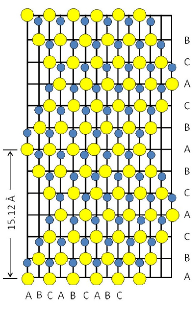
Figure 1: (Color online) Schematic diagram of Si-terminated 6H–SiC(0001). Small blue circles are carbon atoms while the large yellow ones are Si atoms.

and obtain C-rich layers by simply removing the topmost Si-layers, which is a numerical procedure introduced to mimic the sublimation process of Si atoms in the epitaxial growth of graphene. The dimensions of our orthorhombic simulation cell containing the 6H–SiC substrate are $60.07\times 61.36\times 15.12$ Å³ in $x$ (generated with lattice parameter $2.668$ Å), $y$ (generated with lattice parameter $1.54$ Å) and $z$ directions, respectively. Note that the periodic boundary conditions are applied along $x$ and $y$, while a vacuum of $30$ Å is created along the $z$ direction.

In addition to preparing the initial configurations of atoms, a technical point which concerns the growth of multilayer graphene is in order. In removing silicon atoms directly from the 6H–SiC crystalline substrate, one focuses on the number of C-rich layers by properly choosing prescribed distances among C-rich layers and substrate. Consider, for example, four C-rich layers after removing Si atoms from the 6H–SiC crystal. We keep the distance between the substrate and the first-layer C-rich atoms next to it at an original separation of $1.9$ Å. Then, between the next two, i.e. first and second C-rich layers, we make it to lie within $1$ Å or a separation smaller. We set a distance $1.9$ Å between the second and third C-rich layers and resume a separation of $1$ Å again between the third and fourth C-rich layers. Note that the C-rich layers take on the original crystalline structure with Si atoms removed, i.e. a centered hexagonal structure with a C–C bond-length of $2.78$ Å which is longer than $2.65$ Å of Tang et al. [2]. The stringent condition between the C-rich layers and substrate should be strictly obeyed otherwise only a few hexagonal rings are created.

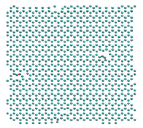
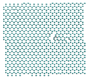
1200 K	1300 K
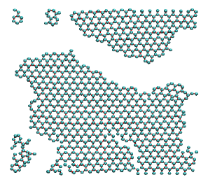
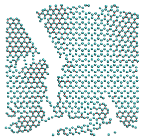
1260 K	1450 K

Figure 2: (Color online) Growth of monolayer graphene on 6H–SiC substrate simulated with TEA (left) and Tersoff (right) potentials. For TEA potential, the threshold annealing temperature at which graphene emerges occurs at a lower temperature within the range $1200<T_{\mathrm{tr}}<1260$ K, whereas it is higher within the range $1300<T_{\mathrm{tr}}<1450$ K for Tersoff potential.

The procedure and the details of parameters used in this simulation growth of graphene on 6H–SiC substrate are summarized as follows:

• We apply the Tersoff and TEA potentials in two separate simulation series to calculate the interatomic C–C and Si-C interactions with parameters given in references [7] and [8], respectively.

• We consider 6H–SiC as a substrate, i.e. six bilayers of Si and C atoms and in each layer of Si or C atoms, a total number of $480$ atoms is considered.

• The simulation procedure is performed by first relaxing the system using the conjugate gradient minimization method [10]. The initial distance of C–C atoms in the C-rich layers after relaxation is $2.78$ Å which is larger than the $2.65$ Å of Tang et al. [2]. Then we perform a MD simulation with a timestep $\Delta t=0.5$ fs, and heat the system until $T=300$ K is reached. In this process, the temperature is increased using a linear ramp within the Nose-Hoover thermostat, so that a heating rate of $10^{13}$ K/s is imposed. At this temperature, the system is equilibrated for a time interval of $2\times 10^{4}\Delta t$. From this configuration, a set of simulations are carried out to increase the temperature of the system to various desired $T$, in order to study the temperature evolution of the carbon layers. As above, a heating rate of $10^{13}$ K/s is chosen. At each target temperature $T$, equilibrium of the system is obtained after a total time interval of $3\times 10^{4}\Delta t$. In the final stage, the system is annealed down to $T=0.1$ K at a cooling rate of $5\times 10^{12}$ K/s so that the properties of the carbon sheets can be studied without thermal noise.

3 Results and discussion

3.1 Growth of monolayer graphene on 6H–SiC substrate

The monolayer graphene simulated with the TEA and Tersoff potentials are compared in figure 2. The main feature to emphasize is the existence of a threshold annealing temperature $T_{\rm tr}$ signaling the emergence of graphene. For the TEA potential, the carbon layers start to transform at 1200 K and the graphene layer is formed at $T_{\rm tr}=1260$ K. The latter is close to the experimentally value observed by Hannon and Tromp [11] who report the formation of smooth steps of graphene in prolonged annealing at 1298 K. For Tersoff’s potential, the transformation of the carbon layers to graphene sheet spreads from 1300 K to the threshold value of 1450 K, which is a more gradual formation of graphene and at a higher temperature than the experiment [11].

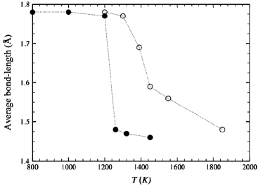
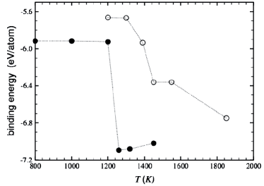
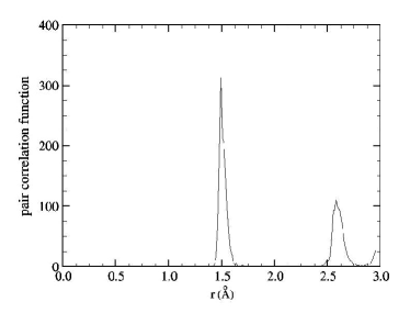
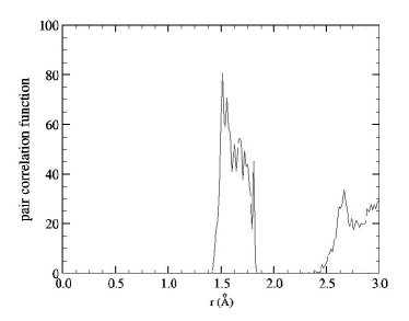
Figure 3: Top row: Comparison of the average C–C bond-length (left) and binding energy (right) of monolayer graphene simulated using the Tersoff (open circle) and TEA (solid circle) potentials. Bottom row: The pair correlation function of graphene obtained by TEA potential (left) at $1260$ K and Tersoff potential (right) at $1450$ K for a monolayer graphene grown on 6H–SiC substrate.

3.2 Bond-length, binding energy, and pair correlation function of monolayer graphene

The concrete evidence that the TEA potential yields a well-defined graphene structure is its prediction of an average C–C bond-length equal to $1.48$ Å (at $1260$ K) (see figures 2 and 3). This value is close to the $sp^{2}$-hybridized graphitic carbon ($1.42$ Å). As for Tersoff’s potential, a value of $1.59$ Å (at $1450$ K) [12] is obtained, which is not as good as the TEA potential. The pair correlation functions $g(r)$ in figure 3 are also consistent with the results of bond-length; the position of the first maximum of $g(r)$ is $1.487$ Å for the TEA potential to be compared with $1.508$ Å for the Tersoff potential. Note in figure 3 that the binding energy for the former potential is $-7.0941$ eV/atom, which is lower than the $-6.3620$ eV/atom obtained from Tersoff’s potential. It is worth mentioning that the binding energies have been calculated directly from the potential energy per carbon atom given by the Tersoff or TEA potential. Armed with these results, our study for two-layer graphene grown on SiC substrate will proceed below by using only the TEA potential.

	1000 K
First layer		Second layer
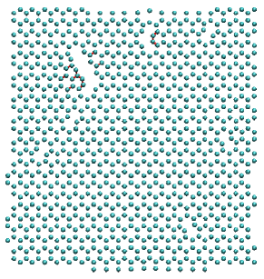
	1320 K
First layer		Second layer

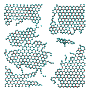
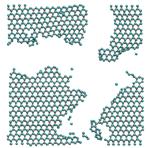
Figure 4: (Color online) Two layers of graphene grown on 6H–SiC substrate simulated with TEA potential. The first-layer graphene corresponds to the one near the substrate.

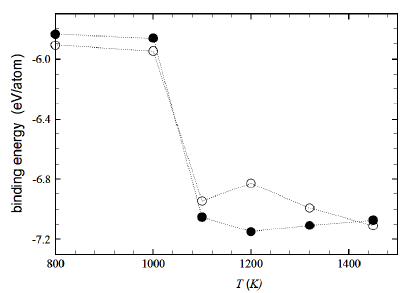
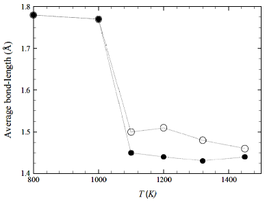
Figure 5: Average bond-length (right) and binding energy (left) for the first (open circle) and second (solid circle) layers graphene grown on 6H–SiC substrate.

3.3 Growth of two-layer graphene on 6H–SiC substrate

Figure 4 shows the two-layer graphene grown on 6H–SiC substrate. The first graphene layer, which is the one that clings to substrate, is relatively less stable than the second layer. This is evident from examining Figure 5 for the bond-length and binding energy for the two layers. The bond-length of the second graphene layer at $T=1320$ K is $1.43$ Å. This value is smaller than $1.48$ Å of the first layer and is closer in magnitude to the $1.42$ Å bond-length of $sp^{2}$-hybridized graphene carbon. Further evidence can be gleaned also from the pair correlation function $g(r)$ at $T=1320$ K whose first maximum position for the first layer is $1.53$ Å to be compared with $1.48$ Å of the second layer. The binding energy of the second layer at $T=1320$ K is estimated to be $-7.1085$ eV/atom which is lower than $-6.9925$ eV/atom for the first layer.

4 Conclusion

We have applied the MD simulation to the study of the growth of graphene on 6H–SiC substrate by epitaxial method. It was found that the choice of an empirical potential in simulation is sensible in predicting the threshold temperature at which point the graphene starts to emerge. With the TEA potential, we obtained one and two layers of graphene grown on 6H–SiC(0001) substrate. In addition to yielding the threshold annealing temperature, which was found to be reasonably close to that implied in recent experiments, the characteristics of the grown graphene are confirmed by the calculated average C–C bond-length, pair-correlation function and binding energy. With this empirical potential in hand, one can envisage investigating the thermal stability of multilayer graphene and carrying out a deeper analysis of growth mechanisms. Works along these lines are in progress.

Рiст графену на 6H–SiC в симуляцiях методом
молекулярної динамiки

Н. Жаксlabel1, Р. Арiфен label2, С.К. Лаilabel2

label1 Нацiональний полiтехнiчний iнститут Ґренобля, Унiверситет Жозефа Фур’є–Нацiональний центр наукових дослiджень, 38402 Сан-Мартен д’Ере, Францiя label2 Лабораторiя складних рiдин, Фiзичний факультет, Нацiональний центральний унiверситет, Чунґлi 320, Тайвань

References

- [1] Peres N.M.R., Ribeiro R.M., New J. Phys., 2009, 11, 095002; doi:10.1088/1367-2630/11/9/095002.
- [2] Tang C., Meng L., Xiao H., Zhong J., J. Appl. Phys., 2008, 103, 063505; doi:10.1063/1.2894728.
-
[3]
Poon S.W., Chen W., Wee T.S., Tok E.S.,
Phys. Chem. Chem. Phys., 2010, 12, 13522;
doi:10.1039/B927452A. -
[4]
Tang C., Meng L., Sun L., Zhang K., Zhong J.,
J. Appl. Phys., 2008, 104, 113536;
doi:10.1063/1.3032895. -
[5]
Varchon F., Mallet P., Veuillen J.Y., Magaud L.,
Phys. Rev. B, 2008, 77, 235412;
doi:10.1103/PhysRevB.77.235412. -
[6]
Lampin E., Priester C., Krzeminski C., Magaud L.,
J. Appl. Phys., 2010, 107, 103514;
doi:10.1063/1.3357297. - [7] Tersoff J., Phys. Rev. B, 1989, 39, 5566; doi:10.1103/PhysRevB.39.5566.
- [8] Erhart P., Albe K., Phys. Rev. B, 2005, 71, 035211; doi:10.1103/PhysRevB.71.035211.
-
[9]
LAMMPS code, http://lammps.sandia.gov.
Plimpton S., J. Comput. Phys., 1995, 117, 1; doi:10.1006/jcph.1995.1039. - [10] Payne M.C., Teter M.P., Allan D.C., Arias T.A., Jonnopoulos J.D., Rev. Mod. Phys., 1992, 64, 1045; doi:10.1103/RevModPhys.64.1045.
- [11] Hannon J.B., Tromp R.M., Phys. Rev. B, 2008, 77, 241404R; doi:10.1103/PhysRevB.77.241404.
- [12] At this temperature only part of the area covers with grown graphene. If we consider K, grown graphene covers the whole area (not shown) with an average C–C bond-length of Å. This annealing temperature differs, however, from ours using TEA potential and is certainly much higher than the experimentally observed value.