Transport properties of the metallic state of overdoped cuprate superconductors from an anisotropic marginal Fermi liquid model

Abstract

We consider the implications of a phenomenological model self-energy for the charge transport properties of the metallic phase of the overdoped cuprate superconductors. The self-energy is the sum of two terms with characteristic dependencies on temperature, frequency, location on the Fermi surface, and doping. The first term is isotropic over the Fermi surface, independent of doping, and has the frequency and temperature dependence characteristic of a Fermi liquid. The second term is anisotropic over the Fermi surface (vanishing at the same points as the superconducting energy gap), strongly varies with doping (scaling roughly with $T_{c}$, the superconducting transition temperature), and has the frequency and temperature dependence characteristic of a marginal Fermi liquid. Previously it has been shown this self-energy can describe a range of experimental data including angle-dependent magnetoresistance (ADMR) and quasi-particle renormalisations determined from specific heat, quantum oscillations, and angle-resolved photo-emission spectroscopy (ARPES). Without introducing new parameters and neglecting vertex corrections we show that this model self-energy can give a quantitative description of the temperature and doping dependence of a range of reported transport properties of Tl2201 samples. These include the intra-layer resistivity, the frequency dependent optical conductivity, the intra-layer magnetoresistance, and the Hall coefficient. The temperature dependence of the latter two are particularly sensitive to the anisotropy of the scattering rate and to the shape of the Fermi surface. In contrast, the temperature dependence of the Hall angle is dominated by the Fermi liquid contribution to the self-energy that determines the scattering rate in the nodal regions of the Fermi surface.

I Introduction

Much research on strongly correlated electron materials, with high-temperature superconducting cuprates being the prominent example, is focused on the experimental or theoretical determination of the relevant electronic self-energy. That is because the self-energy can provide insight into the underlying quantum many-body physics. Proper knowledge of the self-energy in the metallic phase of high-temperature superconductors is also believed to be a step towards solving the mystery of high-temperature superconductivity since ultimately superconductivity is an instability in the metallic state. A model self-energy capable of a unified description of results from many experiments is therefore desirable and provides a benchmark for comparison with microscopic theories based on lattice effective Hamiltonians such as the $t-J$ and Hubbard models.

In the last two decades experimental data has been used to deduce the self-energy, both directly and indirectly. Angle-resolved photoemission spectroscopy (ARPES) offers information on both the real and imaginary part of the self-energy damascelli03 ; valla99 ; valla00 ; kordyuk04 ; kaminski05 ; chang08 ; zhu08 ; plate05 , specific heatwade94 ; loram94 provides information through renormalization effects, and angle-dependent magnetoresistance abdel06 ; abdel07 ; analytis07 ; kennett07 (ADMR) provides information on the imaginary part of the self-energy or scattering rate close to the Fermi level. Further information about the temperature and doping dependence can be obtained from measurements of the resistivity tyler ; tyler98 ; manako92 ; mackenzie96 ; hussey08 , intra-layer magnetoresistance hussey96 and Hall effect manako92 ; mackenzie96 ; hussey08 ; kubo91 ; hussey96 . In addition, the optical conductivity basov05 ; puchkov96 ; ma06 ; basov11 provides information on the frequency dependence of the self-energy.

Previous work kokalj11 introduced a particular model self-energy, motivated by ADMR abdel06 ; abdel07 , that could describe consistently and quantitatively ADMR and a number of quantities determined by the real part of the self-energy, including ARPES dispersion plate05 , specific heat wade94 ; loram94 , and effective masses deduced from quantum oscillations rourke10 , in the entire overdoped regime of Tl₂Ba₂CuO_6+δ (Tl2201). In this paper we extend our analysis to description of transport properties, which are largely determined by the imaginary part of the self-energy. Properties considered include the intra-layer resistivity tyler ; tyler98 ; manako92 ; mackenzie96 , Hall effect manako92 ; mackenzie96 ; kubo91 ; hussey96 , intra-layer magnetoresistance hussey96 , and optical conductivity basov05 ; puchkov96 ; ma06 . We show that all of these can be quantitatively described with our model self-energy without any additional fitting parameters for the entire overdoped regime for Tl2201.

The outline of the paper is as follows. In Section II we review the form of the self-energy and its parametrisation. Section III considers the DC conductivity and the frequency dependent conductivity. It is shown that at high temperatures and frequencies these are sensitive to the cut-off frequency which appears in the Fermi liquid term in the self-energy. In Section IV we show that the Hall coefficient strongly depends on the shape of the Fermi surface and that its non-monotonic temperature dependence gives strong support for our model self-energy. We also argue that the observed non-monotonic temperature dependence of the Hall coefficient cannot be captured with some alternative models, e.g., with the isotropic marginal Fermi Liquid model abrahams03 . We also argue that the observed $T^{2}$ dependence of the Hall angle arises because it is dominated by the isotropic part of the self-energy, which also equals the smallest scattering rate on the Fermi surface in the nodal direction, and that the contribution of the anisotropic part is suppressed. Hence, results on the Hall angle give additional support to our model self-energy, in particular the $T^{2}$ dependence of the isotropic part of self-energy. In Section V we consider the intra-layer magnetoresistance. In Section VI we briefly review relevant results from microscopic model calculations. Although, several are qualitatively consistent with the model self-energy, they tend to obtain scattering rates that are significantly less than observed. Section VII contains some conclusions and suggestions for possible future work.

II Model self-energy

Our model self-energy is motivated by the angle-dependent magnetoresistance (ADMR) experiments on overdoped Tl2201 abdel06 ; abdel07 ; analytis07 , where two distinct scattering rates were uncovered. The first is more Fermi liquid (FL) like and is isotropic over the Fermi surface, weakly doping dependent, and shows $T^{2}$ dependence at low $T$. The second has a marginal Fermi liquidvarma89 ; littlewood91 ; varma02 frequency and temperature dependence and is strongly anisotropic over the Fermi surface (the same anisotropy as the superconducting gap). Its strength follows the doping dependence of $T_{c}$ in the strongly overdoped regime and is linear in $T$ down to the lowest $T$.

Accordingly, our model self-energy can be written,

$$\Sigma^{\prime\prime}({\bf k},\omega)=\Sigma^{\prime\prime}_{\textrm{FL}}(\omega)+\Sigma_{\textrm{AMFL}}^{\prime\prime}(\phi,\omega),$$ (1)

where $\phi$ denotes the position on the Fermi surface (see Fig. 5). The imaginary part of the isotropic FL like self-energy is given by JackoNP09

$$\Sigma_{\textrm{FL}}^{\prime\prime}(\omega)=\left\{\begin{array}[]{ll}-\frac{1}{2\tau_{0}}-s\frac{\omega^{2}+\pi^{2}T^{2}}{\omega_{\textrm{FL}}^{*2}}&\textrm{ for }\frac{\omega^{2}+\pi^{2}T^{2}}{\omega_{\textrm{FL}}^{*2}}\leq 1,\\ \big{[}-\frac{1}{2\tau_{0}}-s\big{]}F\big{(}\frac{\omega^{2}+\pi^{2}T^{2}}{\omega_{\textrm{FL}}^{*2}}\big{)}&\textrm{ for }\frac{\omega^{2}+\pi^{2}T^{2}}{\omega_{\textrm{FL}}^{*2}}>1.\end{array}\right.$$ (2)

Here $1/(2\tau_{0})$ accounts for the impurity scattering, and Matthiessen’s rule is implicitly assumed. The parameter $s$ gives the strength of the FL like self-energy part and $\omega_{\textrm{FL}}^{*}$ is the high-$\omega$ cutoff (see Fig. 1). We use units $\hbar=k_{B}=1$. $\Sigma_{\textrm{FL}}^{\prime\prime}$ is quadratic in $\omega$ and $T$ at low $\omega$ and $T$. The function $F$ is a slowly decreasing function with $F(1)=1$, which we simply approximate with a constant.

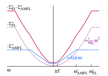
Figure 1: Frequency dependence of the imaginary part of the model self-energy. The first part $\Sigma_{\textrm{FL}}$, is Fermi liquid like, with a quadratic $\omega$ and $T$ dependence, up to the high-$\omega$ cutoff $\omega_{\textrm{FL}}^{*}$, and with a prefactor $s/\omega_{\textrm{FL}}^{*2}$, This part is taken to be doping independent. The second part is the anisotropic marginal Fermi liquid part, whose imaginary part is constant for $\omega<\pi T$ and proportional to $T$, while it is linear in $\omega$ for higher $\omega$ up to a high-$\omega$ cutoff $\omega_{\textrm{AMFL}}^{*}$. Its strength is given by $\lambda(\phi)$, which is strongly anisotropic over the Fermi surface and also strongly doping dependent.

The anisotropic marginal Fermi liquid (AMFL) part of the self-energy (its imaginary part) has the following form,

$$\Sigma_{\textrm{AMFL}}^{\prime\prime}(\phi,\omega)=\left\{\begin{array}[]{ll}\lambda(\phi)(-\frac{\pi}{2}x)&\textrm{ if }|\omega|\leq\omega_{\textrm{AMFL}}^{*},\\ \lambda(\phi)(-\frac{\pi}{2}\omega_{\textrm{AMFL}}^{*})&\textrm{ if }|\omega|>\omega_{\textrm{AMFL}}^{*},\end{array}\right.$$ (3)

where $\lambda(\phi)$ determines its strength and is anisotropic over the Fermi surface, $x=\max(|\omega|,\pi T)$, and $\omega_{\textrm{AMFL}}^{*}$ is the high-$\omega$ cutoff. $\Sigma_{\textrm{AMFL}}^{\prime\prime}(\phi,\omega)$ is linear in $\omega$ and $T$ for low $\omega$ or low $T$ (see Fig. 1). The real part of the self-energy is obtained from a Kramers-Kronig relation and is not explicitly given here. Explicit low $\omega$ behaviour of the real part can be found in Ref. kokalj11, .

Parameters of the model self-energy were already extracted in Ref. kokalj11, for overdoped Tl2201. From ADMR one can estimate that $s/\omega_{\textrm{FL}}^{*2}=9.2$ eV^-1 and

$$\lambda(\phi)=1.6\cos^{2}(2\phi)T_{c}(p)/T_{c}^{\max},$$ (4)

where $T_{c}(p)$ is the doping ($p$) dependent transition temperature and $T_{c}^{\max}$ is the maximal transition temperature. For the doping dependence of $T_{c}$ we use the phenomenological relation tallon95 $T_{c}(p)/T_{c}^{\textrm{max}}=1-82.6(p-0.16)^{2}$ with $T_{c}^{\textrm{max}}=93$ K at the optimal doping $p=0.16$ for Tl2201. This $T_{c}(p)$ relation is for illustrative purposes only since the superconductivity actually survives up to $p=0.31$, as was found in Ref. bangura10, . In addition, $\omega_{\textrm{FL}}^{*}$ was estimatedkokalj11 to be 0.23 eV from specific heat measurements in the highly overdoped and non-superconducting regime. The cutoff $\omega_{\textrm{AMFL}}^{*}$ only weakly influences the results kokalj11 because it only enters the real part of the self energy via a logarithmic dependence and is here taken to be $0.2$ eV. For the Tl2201 samples used in ADMR abdel06 ; french09 the impurity scattering rate was estimated to be, $1/(2\tau_{0})\sim 4$ meV. These parameter values for the model self-energy give a consistent description of several experiments, including ADMR, specific heat, quantum oscillations, and the quasi-particle dispersion seen in ARPES kokalj11 .

For Hubbard models, there is an additional constraint on the self-energy, and in particular its high-frequency behaviour, via the sum rule vilk97

$$\int d\omega(-\Sigma_{\sigma}^{\prime\prime}(k,\omega))=\pi Un_{-\sigma}(1-n_{-\sigma}),$$ (5)

with $U$ being the on site Coulomb interaction strength, and $n_{\sigma}=(1+p)/2$ being the density of electrons with spin $\sigma$. Our model self-energy does not obey this sum rule since $\Sigma^{\prime\prime}(k,\omega)$ stays finite for $\omega\to\infty$. To fulfill the sum rule our $\Sigma^{\prime\prime}(k,\omega)$ should be strongly suppressed at high frequencies. We estimate this suppression should occur at $\omega\sim 5$ eV (for $U=8t$). Such a suppression would not influence our results, since they are determined by the value of the self energy at much lower frequencies. Hence, we do not employ the suppression and the self-energy sum rule in this work. In contrast, in the next Section it is shown that the behaviour of the self-energy near our cutoff frequencies $\omega_{\textrm{FL}}^{*}$ and $\omega_{\textrm{AMFL}}^{*}$ does affect some observed transport properties at high temperatures and frequencies.

For the bare band dispersion $\epsilon_{0}(k)$ we approximate the LDA results in Ref. peets07, with the following hopping parameters. $t_{1}=0.438$, $t_{2}=-0.150$, $t_{3}=0.084$, $t_{4}=-0.013$, $t_{5}=-0.020$, $t_{6}=0.029$, all expressed in eV (for details see Supplemental material of Ref. kokalj11, ). To obtain the Fermi surface volume of the overdoped regime we apply a rigid band shift through the chemical potential $\mu$. The main doping dependence of our results does not come from the band filling, which we therefore keep fixed, but rather from the doping (or $T_{c}$) dependence of the self-energy. Shifting the chemical potential from values appropriate for highly overdoped to optimal doping (e.g., from $p=0.3$ to 0.15) induces only a small change of our results (see Fig. 8 for example).

III Intra-layer Conductivity

The frequency dependent conductivity is approximated with the bubble diagram in which the non-interacting Green’s functions are exchanged with interacting ones and vertex corrections are neglected bruus .

$${\rm Re} \ \sigma_{xx}(\omega)=\frac{2\pi e^{2}}{V}\sum_{\vec{k}}v_{0,x}^{2}(\vec{k})$$ (6)

$$\times\int dy\frac{n_{F}(y)-n_{F}(y+\omega)}{\omega}A(\vec{k},y)A(\vec{k},y+\omega),$$

where $v_{0,x}(\vec{k})$ is the bare band velocity in the $x$ direction at wave vector $\vec{k}$, $n_{F}(y)$ is the Fermi-Dirac distribution function and $A(\vec{k},\omega)$ is the spectral function

$$A(\vec{k},\omega)=-\frac{1}{\pi}{\rm Im}G^{R}(\vec{k},\omega)$$ (7)

where $G^{R}(\vec{k},\omega)$ is the retarded Green’s function.

Our interest is mostly in low $T$ and low $\omega$ properties of the conductivity for which the parameter space close to the Fermi surface is the most relevant (mainly due to the factor $(n_{F}(y)-n_{F}(y+\omega))/\omega$). In this parameter space we can linearize the bare-band dispersion

$$\epsilon_{0}(\vec{k})=\epsilon_{0}(k_{r},\phi)\simeq\epsilon_{F}+v_{0,F,r}(\phi)(k_{F}(\phi)-k_{r}),$$ (8)

where $k_{F}(\phi)$ is a Fermi momentum at angle $\phi$, which is the angle between the $(\pi,\pi)$-$(0,\pi)$ and $(\pi,\pi)$-$k$ directions (Fig. 5). $v_{0,F,r}(\phi)$ is the derivative of the bare band dispersion in the $k_{r}$ direction [i.e., the radial from $(\pi,\pi)$, see Fig. 5]. For a circular Fermi surface $v_{0,F,r}(\phi)$ just corresponds to a Fermi velocity.

By performing the integral over $k_{r}$ the optical conductivity can be approximated for a quasi 2D system with

$${\rm Re}\ \sigma_{xx}(\omega)=\frac{e^{2}}{4\pi^{2}d}\int d\phi\int dy\frac{n_{F}(y)-n_{F}(y+\omega)}{\omega}$$

$$\times\frac{k_{F}(\phi)v_{0,F}^{2}(\phi)}{v_{0,F,r}(\phi)}{\rm Im}\frac{1}{\omega+\Sigma^{R}(\phi,y)-\Sigma^{A}(\phi,y+\omega)}.$$ (9)

$d$ is the distance between CuO layers ($d=11.6$ Å for Tl2201 french09 ), $v_{0,F}(\phi)$ is a Fermi velocity while $\Sigma^{R}(\phi,\omega)$ and $\Sigma^{A}(\phi,\omega)$ are the retarded and advanced self-energies, respectively. We assume that they are only $\phi$-dependent in $\vec{k}-$space (anisotropic over the Fermi surface) in addition to our proposed $\omega$ and $T$ dependencies. In deriving Eq. (9) the integral over $k_{r}$ was extended to [$-\infty$,$\infty$] which is a good approximation for low $T$ and $\omega$ due to the strongly peaked spectral function close to the FS. This means any effects of van Hove singularities or band edges are neglected. Eq. (9) can be viewed as a generalization of Eq. (12) in Ref. basov05, to the case of a $\phi$ dependent self-energy.

The imaginary part of the optical conductivity can be obtained by the Kramers-Kronig transformation,

$${\rm Im}\ \sigma_{xx}(\omega)=-\frac{1}{\pi}\mathcal{P}\int_{-\infty}^{\infty}\frac{{\rm Re}\ \sigma_{xx}(\omega^{\prime})}{\omega^{\prime}-\omega}d\omega^{\prime},$$ (10)

or by generalizing Eq. (9) to the complex conductivity

$$\sigma_{xx}(\omega)=\frac{{\rm i}e^{2}}{4\pi^{2}d}\int d\phi\int dy\frac{n_{F}(y)-n_{F}(y+\omega)}{\omega}$$

$$\times\frac{k_{F}(\phi)v_{0,F}^{2}(\phi)}{v_{0,F,r}(\phi)}\frac{1}{\omega+\Sigma^{A}(\phi,y)-\Sigma^{R}(\phi,y+\omega)}.$$ (11)

The plasma frequency $\omega_{p}$ is determined by the high frequency behaviour ($\omega\gg$ band width),

$$\omega_{p}^{2}\equiv\frac{1}{\epsilon_{0}}{\rm lim}_{\omega\to\infty}\ \omega{\rm Im}\ \sigma_{xx}(\omega)$$ (12)

and in our case this quantity is given by the following integral over the Fermi surface

$$\omega_{p}^{2}=\frac{e^{2}}{4\pi^{2}d\epsilon_{0}}\int d\phi\frac{k_{F}(\phi)v_{0,F}(\phi)^{2}}{v_{0,F,r}(\phi)}.$$ (13)

The above expression is equivalent to the band theory expression ashcroft ,

$$\omega_{p}^{2}=\frac{e^{2}}{\epsilon_{0}}\int\frac{d^{3}k}{4\pi^{3}}n_{F}(\epsilon_{0}(k))\frac{\partial^{2}\epsilon_{0}(k)}{\partial k_{x}^{2}}.$$ (14)

This equivalence can be shown by integrating by parts, confining the integral to the Fermi surface due to derivative of a Fermi function and then using the symmetry $\sigma_{xx}=\sigma_{yy}$. Here $\epsilon_{0}$ is the static dielectric constant.

Using these expressions with our bare band dispersion (see Section II) we obtain $\omega_{p}\simeq 23000$ cm^-1, while in Ref. puchkov96, they experimentally obtain $\omega_{p}\sim 15100$ cm^-1 by integrating ${\rm Re}\sigma(\omega)$ up to $\sim 8000$ cm^-1. We believe that this is not a high enough frequency to fully exhaust the sum rule.

III.1 DC conductivity

In the limit of $\omega\to 0$ further simplifications can be made,

$$\frac{1}{\omega+\Sigma^{R}(\phi,y)-\Sigma^{A}(\phi,y+\omega)}\to\frac{1}{2{\rm i}\Sigma^{\prime\prime}(\phi,y)},$$ (15)

where $\Sigma^{\prime\prime}(\phi,y)$ stands for imaginary part of the retarded self-energy. Furthermore,

$$\frac{n_{F}(y)-n_{F}(y+\omega)}{\omega}\to-\frac{\partial n_{F}(y)}{\partial y}.$$ (16)

The DC conductivity can then be written as

$${\rm Re}\sigma_{xx} = \frac{e^{2}}{4\pi^{2}d}\int d\phi\frac{k_{F}(\phi)v_{0,F}^{2}(\phi)}{v_{0,F,r}(\phi)}$$ (17)

$$\times\int dy(-\frac{\partial n_{F}(y)}{\partial y})\frac{1}{-2\Sigma^{\prime\prime}(\phi,y)}.$$

For the bare band dispersion appropriate to Tl2201 the pre-factor $\frac{k_{f}(\phi)v_{0,F}(\phi)^{2}}{v_{0,F,r}(\phi)}$ turns out to be relatively constant with $\phi$ (variation $<$20%). In comparison the anisotropy of the self-energy ($1/\Sigma^{\prime\prime}$ can vary by a factor of more than two) and so the pre-factor can therefore be taken out of the integral, replaced with its average value and expressed in terms of $\omega_{p}$ [Eq. (13)]. With this approximation we can rewrite the expression for the frequency dependent conductivity in Eq. (11) in a similar form to Equation (12) in Ref. basov05, ,

$$\sigma_{xx}(\omega)=\frac{{\rm i}\omega_{p}^{2}\epsilon_{0}}{2\pi}\int dy\frac{n_{F}(y)-n_{F}(y+\omega)}{\omega}$$

$$\times\int d\phi\frac{1}{\omega+\Sigma^{A}(\phi,y)-\Sigma^{R}(\phi,y+\omega)}.$$ (18)

Using the $\cos^{2}(2\phi)$ dependence of our model self-energy, one can perform the integral over $\phi$ in the Eq. (18) for $\omega=0$. At this point only the integral over the frequency $y$ remains, which can be to the lowest order at low $T$ calculated with the use of

$$-\frac{\partial n_{F}(y)}{\partial y}\to\delta(y).$$ (19)

This is a good approximation, if the self-energy (or $1/\Sigma^{\prime\prime}$) is a fairly constant function of $\omega$ for $|\omega|\lesssim T$. However, further improvements can be made by expanding the self-energy part to $y^{2}$ term and then numerically approximating the $y$ integral by Pade approximation, which gives errors less than $10^{-6}$.

The resulting expression allows us to perform fits of the measured resistivity ($\rho_{xx}=1/{\rm Re}\sigma_{xx}$) using the three main parameters of our model: the strength of impurity scattering $1/(2\tau_{0})$, the strength of AMFL part of self-energy $\lambda$ [where $\lambda(\phi)\equiv\lambda\cos^{2}(2\phi)$], and the strength of FL part of self-energy $s/\omega_{\textrm{FL}}^{*2}$.

The resulting fits for various Tl2201 samples with different $T_{c}$s are shown in Fig. 2.

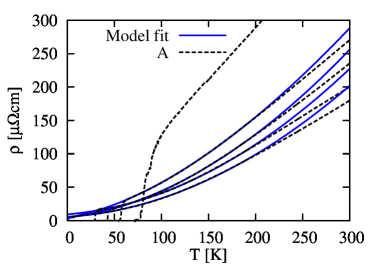
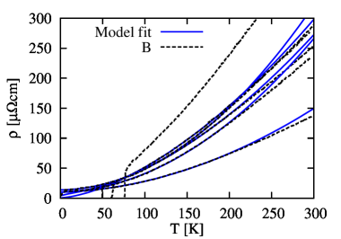
Figure 2: Comparison of the measured temperature dependence of the intra-layer resistivity $\rho_{xx}$ to fits for the self-energy model. Fits are performed in the $T$ range from above $T_{c}$ to 200 K and agree nicely with the data. At higher $T>200$ K our model predicts a stronger increase in $\rho_{xx}$, which could be improved by smoother high frequency cutoffs in the self-energy. This would introduce new parameters and is beyond the scope of this paper. $T_{c}$ values and references for the data denoted with A and B are given in Table 1.

Table 1: Experimental data sets for the temperature dependence of the DC intra-layer resistivity which are fit to our self-energy model. (Compare Figures 2 and 3). The corresponding $T_{c}$’s and references are listed.

Data identifier	Data $T_{c}$ [K]	Reference
A	0, 30, 43, 57, 83	A.W. Tyler et al., Ref. tyler,
B	0, 7, 10, 48, 63, 76	T. Manako et al., Ref. manako92,
C	15	A.P. Mackenzie et al., Ref. mackenzie96,
D	30, 80	A.W. Tyler et al., Ref. tyler98,

Fits to the optimal doping data are not performed since they yield unphysical values of the parameters (e.g., values of $1/\tau_{0}\sim 0$). This is due to the strong increase of the resistivity at optimal doping and is probably related to the opening of the pseudogap or some other new physics, which is beyond the scope of our model self-energy.

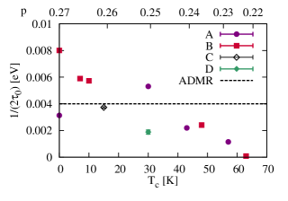
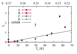
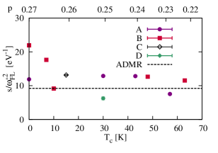
Figure 3: Doping ($p$) or transition temperature ($T_{c}$) dependence of the model parameters extracted from fitting the temperature dependence of the resistivity for a range of Tl2201 samples. The fitted model parameters are consistent with the values and doping dependencies extracted from ADMR kokalj11 . Strength of the impurity scattering $1/(2\tau_{0})$ shows additional decreasing trend with decreasing doping, which might be due to a smaller amount of doped interstitial oxygen. The AMFL strength $\lambda$ shows a strong increase with decreasing doping in good agreement with the results from ADMR kokalj11 . Good agreement with the self-energy model is also found for the doping independent strength of the FL like scattering $s/\omega_{\textrm{FL}}^{*2}$. For the doping dependence of $T_{c}$ we use the phenomenological relation (see section II). $T_{c}$ values and references for the data denoted with A, B, C and D are given in Table 1.

The resulting fit parameters together with the ones extracted from ADMR are shown in Fig. 3. All parameters are consistent with the ones extracted from ADMR kokalj11 . The zero-temperature scattering rate $1/(2\tau_{0})$ seems to show an additional decreasing trend with increasing $T_{c}$, which might be attributed to the loss of interstitial oxygen causing impurity scattering. The anisotropic marginal Fermi liquid parameter $\lambda$ increases with $T_{c}$ as expected, although it suggests a super-linear increase for $T_{c}$ close to the optimal doping. The parameter $s/\omega_{\textrm{FL}}^{*2}$ is slightly larger than extracted from ADMR but still fairly constant with doping. Similar results were also obtained from the conductivities of overdoped LSCO cooper09 .

Fitting parameters for $T_{c}>70$ K become unphysical (too small $1/\tau_{0}$) and might be a sign of a new physics out of the scope of our simple model self-energy.

We found that the resulting fit parameter values do not change significantly if only the zero frequency self-energy is taken into account, as occurs with the delta function approximation for the Fermi-function term, Eq. (19).

For higher temperatures the measured resistivity shows a linear in $T$ dependence over a broader temperature region than our model (Fig. 2). As discussed further below, a smoother saturation of the self-energy at high $T$ and high $\omega$ may improve the comparison in this regime.

Saturation of the self-energy may originate in the Mott-Ioffe-Regel (MIR) limit at which the mean free path $l=v_{F,0}/(-2\Sigma^{\prime\prime}_{\textrm{max}})$ becomes comparable to the lattice constant and electrons become incoherent. Estimate of $-\Sigma^{\prime\prime}_{\textrm{max}}$ from the MIR limit and our LDA estimate of $v_{F,0}\sim 1a$ [eV] gives $-\Sigma^{\prime\prime}_{\textrm{max}}\sim 0.5$ eV. This is in good agreement with our maximal value of the FL part of self-energy (the main contribution at high $T$) which is $\sim 0.5$ eV. The MIR limit was already successfully applied to the scattering rate saturation of the optimal and overdoped cuprates hussey03a . It is important to mention, that in the underdoped regime, the resistivity saturates at a much larger value than expected from the MIR limit, which may be due to the smaller carrier concentration gunnarsson03 .

III.2 Optical Conductivity

Experiments do not directly measure the frequency dependent conductivity but rather the reflectivity or absorption of a thin film or single crystal. The real and imaginary parts of the conductivity are then extracted from a Kramers-Kronig analysis dressel . This is only stable and reliable if there is experimental data out to sufficiently high frequencies. Furthermore, to aid the physical interpretation of the results experimentalists often plot the frequency dependent scattering rate and effective mass that is deduced from an extended Drude model basov05 . However, this also requires a knowledge of the plasma frequency $\omega_{p}$ (compare Eq. (12)). As mentioned earlier, the bare band dispersion from LDA predicts $\omega_{p}\sim 23000$ cm^-1 a value which is larger than extracted from experiments (15100 cm^-1 in Ref. puchkov96, ).

To simplify the analysis and avoid the introduction of new parameters we compare the results for the model self-energy directly to the measured reflectivity. The reflectivity [$R(\omega)$] or absorption [$A(\omega)=1-R(\omega)$] may be written in terms of the optical conductivity dressel

$$R(\omega)=\frac{1+\frac{1}{\epsilon_{0}\omega}|\sigma_{xx}(\omega)|-\sqrt{\frac{2}{\epsilon_{0}\omega}\big{[}|\sigma_{xx}(\omega)|-{\rm Im}\sigma_{xx}(\omega)\big{]}}}{1+\frac{1}{\epsilon_{0}\omega}|\sigma_{xx}(\omega)|+\sqrt{\frac{2}{\epsilon_{0}\omega}\big{[}|\sigma_{xx}(\omega)|-{\rm Im}\sigma_{xx}(\omega)\big{]}}},$$ (20)

in the limit ${\rm Im}\sigma_{xx}(\omega)\gg\epsilon_{0}\omega$, which is valid in the frequency region of the data. Here $|\sigma_{xx}(\omega)|=([{\rm Re}\sigma_{xx}(\omega)]^{2}+[{\rm Im}\sigma_{xx}(\omega)]^{2})^{1/2}$.

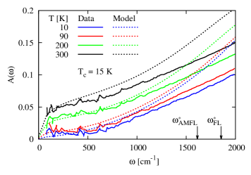
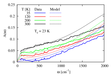
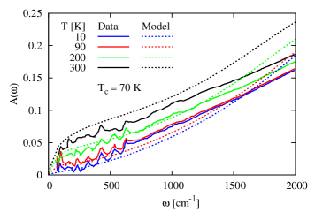
Figure 4: Comparison of the measured optical absorption spectra $A(\omega)$ for Tl2201 at three different dopings with the model self-energy. The latter is for parameter values extracted from ADMRkokalj11 . A good description of the $\omega$, $T$ and $T_{c}$ dependencies of $A(\omega)$ is obtained for $\omega\lesssim 1000$ cm^-1. For higher $\omega$, $A(\omega)$ shows a stronger increase with $\omega$, which could be improved with a softer high-$\omega$ cutoff for the self-energy. This is similar to what is found for the high-$T$ DC resistivity in Fig. 2. Data for $T_{c}=$ 15 K and 70 K are from Ref. ma06, and data for $T_{c}=23$ K are from Ref. puchkov96, .

Comparison of our results, obtained with Eqs. (20) and (18) and model self-energy parameters extracted from ADMR kokalj11 , with the measured absorption is shown in Fig. 4. Agreement at low frequencies ($\omega\lesssim 1000$ cm^-1) is quite satisfactory. We consider this is quite impressive given that no additional fitting parameters beyond those extracted from ADMRkokalj11 have been introduced.

At higher frequencies our model self-energy predicts an absorption that is too large compared to experimental data. This discrepancy could be fixed by incorporating a smoother high-frequency saturation making the self-energy more slowly increasing with $\omega$ and rounding its behaviour at the high frequency cutoff ($\omega_{\textrm{AMFL}}^{*}\simeq\omega_{\textrm{FL}}^{*}\simeq 1700$ cm^-1, see Fig. 4). One way of smoothing the high $T$ and $\omega$ behavior could be in adopting the phenomenological approach of Refs. hussey03a, ; hussey06, , where the saturation of the scattering rate is applied by the ”parallel-resistor” formula, which means the imaginary part of the self-energy (1) is replaced according to

$$\frac{1}{\Sigma^{\prime\prime}_{\textrm{eff}}(\phi,T,\omega)}=\frac{1}{\Sigma^{\prime\prime}_{\textrm{ideal}}(\phi,T,\omega)}+\frac{1}{\Sigma^{\prime\prime}_{\textrm{max}}}.$$ (21)

Here $\Sigma^{\prime\prime}_{\textrm{ideal}}(\phi,T,\omega)$ is the self-energy without high-frequency cutoffs and $\Sigma^{\prime\prime}_{\textrm{max}}$ is the maximal or saturated value of the imaginary part of self-energy, and can be treated as a free parameter. In the MIR picture described above this parameter is estimated to have a value $\sim\hbar v_{F}/a$, where $a$ is the lattice constant.

Using two different model self-energies Norman and Chubukov norman06 performed a detailed analysis of the frequency dependent conductivity for optimally doped Bi₂Sr₂Ca_0.92Y_0.08Cu₂O_8+δ. They deduced a flattening of the frequency dependence of the scattering rate near a cutoff energy of order 0.3 eV. The high-frequency cutoff may also be observed in ARPES as a kink or ”waterfall” in the QP dispersion due to a noticeable change in $\partial\Sigma^{\prime}/\partial\omega$, particularly if it obtains a value $\gtrsim 1$ (for example see Refs. chang08, ; zhu08, ).

The cutoffs give some insight into the underlying physics since they tell us the energy scales of the excitations (e.g., spin fluctuations, particle-hole excitations) which the electrons are scattering off norman06 . On the other hand, cutoffs may also reflect the limiting scattering rate (e.g., given by the sum rule Eq. (5) or the entry into the MIR limit hussey03a ; gunnarsson03 ) or entrance into the incoherent regime.

IV Hall effect

IV.1 Hall coefficient

The Hall coefficient in the weak field limit is given by

$$R_{H}=\frac{\sigma_{xy}^{(1)}}{B_{z}[{\rm Re}\sigma_{xx}]^{2}},$$ (22)

where $B_{z}$ is the magnetic field in the $z$ or $c$ direction, $\sigma_{xy}^{(1)}$ is the Hall conductivity proportional to $B_{z}$, and ${\rm Re}\ \sigma_{xx}$ is the in-plane DC conductivity (see Sec. III.1).

A diagrammatic calculation of the Hall conductivity is given in Ref. kohno88, , leading to

$$\sigma_{xy}^{(1)}=\frac{-{\rm i}eB_{z}}{2}\sum_{k}\int\frac{d\omega}{2\pi}(-\frac{\partial n_{F}(\omega)}{\partial\omega})[J_{x}\tilde{\partial}_{y}J_{y}][G^{R}\tilde{\partial}_{x}G^{A}],$$ (23)

where $[A\tilde{\partial}_{\mu}B]=A\partial_{k_{\mu}}B-(\partial_{k_{\mu}}A)B$, $J_{\mu}$ is a current vertex which we approximate with $-ev_{0,\mu}$ by neglecting the vertex corrections, and $G^{R(A)}$ is the retarded (advanced) Green’s functions.

The expression in Eq. (23) for the Hall conductivity can be further simplified with the following approximations. First, we neglect the term $\partial_{k_{x}}\Sigma^{\prime}(k,\omega)$, which arises from differentiation of the Green’s function and is present also as a first trivial correction to the vertex, which we also neglect. We find that calculations with this correction do not significantly change the results, because our $\Sigma^{\prime}(k,\omega)$ is odd-in-$\omega$. Then we linearize the dispersion in the $k_{r}$ direction around the Fermi surface, Eq. (8), and approximate the integral over $k_{r}$, as was similarly done for the DC conductivity (Sec. III.1). Using the symmetry $\sigma_{xy}^{(1)}=-\sigma_{xy}^{(1)}$ and manipulations similar to those of Ong in Ref. ong91, leads to

$$\sigma_{xy}^{(1)}=\frac{e^{3}B_{z}}{4\pi^{2}d}\int d\phi[-{\bf v}_{0,F}(\phi)\times\partial_{\phi}{\bf v}_{0,F}(\phi)]_{z}$$

$$\times\int d\omega(-\frac{\partial n_{F}(\omega)}{\partial\omega})\frac{1}{(-2\Sigma^{\prime\prime}(\phi,\omega))^{2}},$$ (24)

where we have also used that our self-energy depends only on $\phi$ in momentum space. A more detailed derivation can be found in Appendix B.

IV.2 Comparison with the Boltzmann equation

Ong has given an elegant geometrical interpretation of the Hall conductivity $\sigma_{xy}$ for a two-dimensional Fermi liquidong91 . It is proportional to the area swept out by the scattering length or mean-free path ${\bf l}(\phi)\equiv{\bf v}_{F}(\phi)\tau(\phi)$ as one traverses the Fermi surface. This illustrates how the Hall effect is sensitive to anisotropy in the Fermi surface via the Fermi velocity ${\bf v}_{F}(\phi)$ and and to anisotropy in the scattering time $\tau(\phi)$.

Eq. (24) is consistent with the expression derived from the Boltzmann equation hussey03a and with Ong’s geometric expressionong91 . If the frequency dependence of the self-energy close to $\omega=0$ is neglected, then

$$\int d\omega(-\frac{\partial n_{F}(\omega)}{\partial\omega})\frac{1}{(-2\Sigma^{\prime\prime}(\phi,\omega))^{2}}\simeq\frac{1}{(-2\Sigma^{\prime\prime}(\phi,0))^{2}}.$$ (25)

To make the comparison with the Boltzmann equation and relaxation time approximation more explicit, we start with the Boltzmann equation result for the Hall conductivity hussey03a ,

$$\sigma_{xy}^{(1)}=\frac{e^{3}}{2\pi^{2}d}\int d^{2}k(-\frac{\partial n_{F}(E_{k})}{\partial E_{k}})\frac{v_{x}}{\Gamma}{\bf v}\times{\bf B}\cdot{\bf\nabla}(\frac{v_{y}}{\Gamma}).$$ (26)

Here $E_{k}$ is the quasi-particle (QP) dispersion, ${\bf v}=(v_{x},v_{y})$ is the QP velocity, and $\Gamma$ is the scattering rate, which are all $k$-dependent. The integral goes over the first Brillouin zone in two dimensions. Symmetrizing the expression with the use of $\sigma^{(1)}_{xy}=-\sigma^{(1)}_{yx}$ and applying

$$\frac{v_{x}}{\Gamma}{\bf v}\times{\bf B}\cdot{\bf\nabla}(\frac{v_{y}}{\Gamma})={\bf v}\times{\bf B}\cdot(\frac{1}{\Gamma}{\bf\nabla}(\frac{v_{x}v_{y}}{\Gamma})-\frac{v_{y}}{\Gamma^{2}}{\bf\nabla}(v_{x})),$$ (27)

leads to the following expression,

$$\sigma_{xy}^{(1)}=\frac{e^{3}}{4\pi^{2}d}\int d^{2}k(-\frac{\partial n_{F}(E_{k})}{\partial E_{k}}){\bf v}\times{\bf B}$$

$$\cdot(v_{x}{\bf\nabla}(v_{y})-v_{y}{\bf\nabla}(v_{x}))\frac{1}{\Gamma^{2}}.$$ (28)

Furthermore, if the integral over the 2D Brillouin zone is decomposed into the integrals over $\phi$ and $k_{r}$ and in addition the QP dispersion is linearized close to the Fermi surface with $E_{k}\simeq v_{F,r}(\phi)(k_{F}(\phi)-k_{r})$ and $\Gamma\simeq\Gamma(\phi)$, then the integral over $k_{r}$ may be performed (neglecting band edge effects) and we are left only with the integral over $\phi$. For the magnetic field in the $z$ direction one can then rewrite $\sigma_{xy}^{(1)}$ in a similar form as in Eq. (24) if the integral over $\omega$ in Eq. (24) is replaced with $\frac{1}{\Gamma(\phi)^{2}}$ (similar to Eq. (25)). We should note here that the expression derived from the Boltzmann equation includes only renormalized quasi-particle entities, while Eq. (24) includes only non-renormalized quantities. This is not a problem since the renormalization cancels by taking $v_{F}=Zv_{0,F}$ and $\Gamma=-2Z\Sigma^{\prime\prime}$. However, this might not be the case, if the shape of the non-interacting Fermi surface is changed due to the renormalization. This does not happen for our model self-energy, since its real part is always zero at $\omega=0$ due to the imaginary part being an even function of frequency.

The relationship to Ong’s geometric interpretation is more straight forward. If the integral over $\omega$ in Eq. (24) is approximated as in Eq. (25), one can write

$$\sigma_{xy}^{(1)} = \frac{-e^{3}B_{z}}{4\pi^{2}d}\int d\phi[{\bf l}(\phi)\times\partial_{\phi}{\bf l}(\phi)]_{z},$$ (29)

where

$${\bf l(\phi)}={\bf v}_{0,F}(\phi)/[-2\Sigma^{\prime\prime}(\phi,0)]$$ (30)

is the mean free path used in the Ong’s geometrical interpretation of the Hall conductivity. From this expression it is nicely seen that the renormalization $Z$ cancels and that the Hall conductivity is determined by the mean free path on the Fermi surface.

IV.3 Comparison with experiment

The zero temperature ($T=0$) value of the Hall coefficient $R_{H}$ for a circular Fermi surface corresponds to $1/(en_{e})$ with $n_{e}$ being the density of electrons. Deviations from this value depend on the shape of the Fermi surface. If for our tight-binding band structure we assume a rigid band shift from the highly overdoped to optimally doped regime, then the $T=0$ value of $R_{H}$ is expected to change by less than 10%. Temperature broadening affects ${\rm Re}\sigma_{xx}$ and $\sigma_{xy}^{(1)}$ only at higher $T$ and is within our model estimated to result in a relative change of $\sim 10\%$ at $T\sim 200$ K. The $T$ broadening effect is reduced in $R_{H}$ and is estimated to be $\lesssim 0.5\times 10^{-10}$ m${}^{3}/$C. In contrast to the above relatively small changes with temperature and doping, experiment shows that $R_{H}(T)$ can vary by as much as 100%, as $T_{c}$ varies from 0 to 50 K in the overdoped regime (compare Figure 7).

As can be seen from Eq. (24) for $\sigma_{xy}^{(1)}$ and Eq. (17) for ${\rm Re}\sigma_{xx}$ the temperature dependence of the Hall coefficient comes from the $T$-dependence of the anisotropy of the scattering rate. This becomes more apparent if we rewrite the Hall coefficient in the following form

$$R_{H}=\frac{\int d\phi f_{H}(\phi)\frac{1}{(-2\Sigma^{\prime\prime}(\phi))^{2}}}{[\int d\phi f_{DC}(\phi)\frac{1}{(-2\Sigma^{\prime\prime}(\phi))}]^{2}},$$ (31)

where we have neglected the $T$-broadening effects. $f_{H}(\phi)$ is the $\phi$ dependent coefficient (corresponding to the Hall conductivity), which needs to be integrated over $\phi$ and depends only on bare-band dispersion. $f_{DC}(\phi)$ is similar to $f_{H}(\phi)$, but for the DC conductivity (see Appendix A). The only $T$-dependent quantity in the above equation is the self-energy and its $T$-dependent anisotropy is responsible for $T$-dependent $R_{H}$. This is in agreement with results in Ref. stojkovic97, . However, the absolute change of $R_{H}$ with temperature depends strongly on the shape of the Fermi surface. This is demonstrated in Figs. 5 and 6.

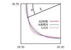
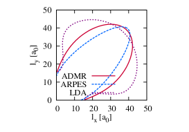
Figure 5: (Left) Three different approximations for the shape of the Fermi surface (FS). The FS deduced from ADMR measurements abdel07 , ARPES measurements plate05 , and tight-binding approximation to the LDA calculations peets07 ; kokalj11 are denoted with ADMR, ARPES, and LDA, respectively. (Right) Curves of the mean-free path ${\bf l}(\phi)$ as one goes around the FS for the three different FSs. According to Ong’s geometric interpretation ong91 the encircled area is proportional to $\sigma_{xy}^{(1)}$ [Eq. (29)]. Although the shapes of the FSs do not change much between different approximations, the mean-free paths and the encircled areas in ${\bf l}$ space change substantially. The main difference comes from the curvature of the FS ($\partial_{\phi}{\bf v}_{0,F}(\phi)$) close to $\phi\sim\pi/8$. The absolute value of $R_{H}$ is therefore very sensitive to the shape of the FS. The mean-free path ${\bf l(\phi)}$ was calculated with our model self-energy for $T=100$ K, and $T_{c}=30$ K.

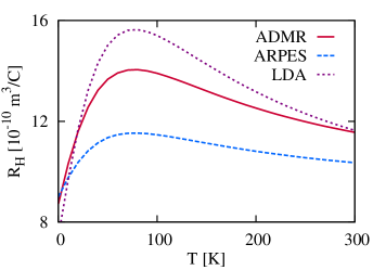
Figure 6: Calculated temperature dependence of the Hall coefficient ($R_{H}$) for three slightly different Fermi surfaces (see Fig. 5). The absolute change or maximal value of $R_{H}$ depends strongly on the shape of the Fermi surface. All curves are calculated with the same scattering rate, using our self-energy model for $T_{c}=30$ K. Temperature broadening effects due to the Fermi-Dirac distribution are not taken into account since they are small ($<10$%). The slightly different values of $R_{H}$ at $T=0$, where the scattering is dominated by impurities and is therefore isotropic, also comes from small changes in the Fermi surface shape.

The overall doping (or $T_{c}$) and $T$ dependence of the measured and calculated $R_{H}$ are shown in Fig. 7 and 8, respectively.

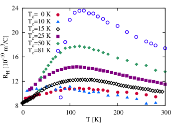
Figure 7: Temperature dependence of the measured Hall coefficient $R_{H}$ for several different $T_{c}$s. These all correspond to dopings for which there is a large hole Fermi surface and show a non-monotonic temperature dependence that increases with increasing $T_{c}$. For $T\lesssim T_{c}$ $R_{H}$ may be strongly suppressed by the superconducting transition. Data for $T_{c}=$ 0 K and 81 K are for polycrystalline samples measured in Ref. kubo91, , data for $T_{c}=$ 10 K and 50 K are from Ref. manako92, , $T_{c}=$ 15 K data is from Ref. mackenzie96, , and $T_{c}=$ 25 K data is from Ref. hussey96, .

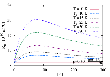
Figure 8: Temperature dependence of the Hall coefficient $R_{H}$ calculated with our model self-energy for several $T_{c}$s and for the ADMR Fermi surface abdel07 . Results should be compared with Fig. 7. The figure illustrates how decreasing doping (increasing $T_{c}$ or $\lambda$ or anisotropy of the self-energy) leads to a large change in the magnitude of the temperature dependence. All results are obtained for the same Fermi surface and only the anisotropy of the self-energy is changed. Arrows shown in the lower right indicate the weak dependence on the band structure change with doping, indicating the absolute shift of the zero temperature value of $R_{H}$ ($T_{c}=0$) for two different dopings ($p=0.15$ and $p=0.30$) as given by a rigid band shift.

The temperature dependence of $R_{H}$ suggests, that the scattering anisotropy strongly (linearly) increases at low $T$ (in our model due to the AMFL part of self-energy), reaches its maximum at $\sim 110$ K and then the scattering slowly becomes more isotropic again as the FL part of the self-energy model begins to dominate.

The fact that for $T_{c}=0$ the experimental $R_{H}$ shows a small $T$-dependence (see Fig. 7) represents a problem for our model, since the model has no anisotropy for $T_{c}=0$. However, there was no ADMR data for $T_{c}=0$ and so it is possible that the anisotropy actually does not go to 0 as $T_{c}\to 0$, or perhaps that our assumption that the $T^{2}$ term is strictly isotropic needs to be relaxed.

Comparison of our results (Fig. 8) with the measured $R_{H}$ (Fig. 7) shows qualitative, and to some extent also quantitative, agreement. However, our $R_{H}$ does reach a maximum for $T\sim 80$ K, while the maximum appears at higher T ($\sim 110$ K) in experiment (Fig. 7). In order to get a better comparison the FL part of our self-energy model should be reduced (smaller $s/\omega_{\textrm{FL}}^{*2}$). Also inclusion of a smoother high frequency cutoff could move the maximum in our $R_{H}(T)$ to higher $T$.

In fitting our model to $R_{H}$ it turns out that one parameter is free (one of $1/(2\tau_{0})$, $\lambda$ or $s/\omega_{\textrm{FL}}^{*}$). This is because the absolute value of $R_{H}$ is unchanged by a re-scaling of the scattering time, as can be seen from Eq. (31). This is closely related to $R_{H}$ not depending on $\tau$ in a simple FL picture.

IV.4 Hall angle

The Hall angle is defined by

$$\cot\theta_{H}(T)\equiv\frac{{\rm Re}\sigma_{xx}}{\sigma_{xy}^{(1)}}=\frac{\rho_{xx}(T)}{R_{H}(T)B_{z}}.$$ (32)

Since our model can describe the temperature dependence of the intra-plane resistivity and Hall coefficient, as we showed above, it must also describe the Hall angle. Here, we examine the temperature dependence of $\cot\theta_{H}$ in order to point out that the observed $T^{2}$ dependence of $\cot\theta_{H}$ (cf. Figure 9) naturally follows from our model self-energy and that there is therefore no need to evoke more exotic theories in order to explain the qualitatively distinct temperature dependence of $\rho_{xx}$ and $\cot\theta_{H}$.

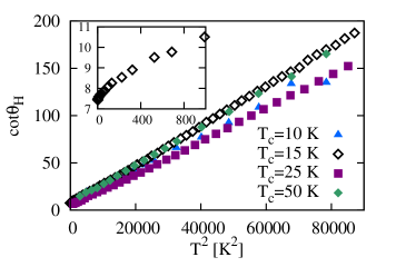
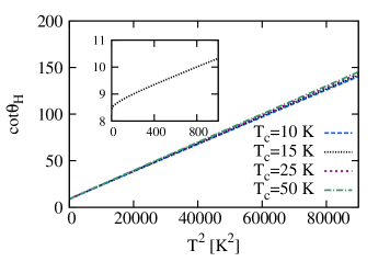
Figure 9: Temperature dependence of the Hall angle $\cot\theta_{H}$. (Top) Experimental data show that $\cot\theta_{H}$ has a linear dependence on $T^{2}$ and a weak doping dependence. A similar dependence is found for our model (Bottom), where the linear dependence of $\cot\theta_{H}$ on $T^{2}$ comes predominantly from the Fermi liquid like scattering ($\Sigma^{\prime\prime}_{\textrm{FL}}$) that gives the scattering rate on the nodal part of the Fermi surface (which also gives the dominant contribution to the Hall conductivity, see Fig. 5). (Top) The Inset shows a small down-turned deviation from the $T^{2}$ dependence of $\cot\theta_{H}$ at low $T$ (for $T_{c}=15$ K). This is also obtained within our model (bottom inset), although not as pronounced as in the experimental data. Experimental data for $T_{c}=$ 10 K and 50 K are from Ref. manako92, . $T_{c}=$ 15 K data is from Ref. mackenzie96, and $T_{c}=$ 25 K data is from Ref. hussey96, . Our model results are calculated with the ADMR Fermi surface.

Experimental data and our results are shown in Fig. 9 and provide additional support for our model self-energy. In particular, the linear dependence of $\cot\theta_{H}$ on $T^{2}$ supports the $T^{2}$ dependence of the isotropic part of self-energy or scattering rate in the nodal direction. That is because $\cot\theta_{H}$ is dominated by the isotropic part ($\Sigma^{\prime\prime}_{\textrm{FL}}$), while it suppresses the anisotropic part ($\Sigma^{\prime\prime}_{\textrm{AMFL}}$) of the self-energy. This point was previously emphasized by Carrington et al.,carrington92 Ioffe and Millis ioffe98 and by Stojkovic and Pines stojkovic97 (see also Ref. fruchter07, ). To show this more explicitly, we use a similar expression to the one in Eq. (31), approximate $f_{H}(\phi)$ and $f_{DC}(\phi)$ with a constant, and perform the integrals over $\phi$. This leads to

$$\cot\theta_{H}\propto-\Sigma_{\textrm{FL}}^{\prime\prime}(0)[1+\frac{\Sigma_{\textrm{FL}}^{\prime\prime}(0)}{\Sigma_{\textrm{FL}}^{\prime\prime}(0)+\Sigma_{\textrm{AMFL}}^{\prime\prime}(0,0)}]^{-1}.$$ (33)

It turns out that the temperature dependence of $\cot\theta_{H}$ is dominated by the first factor, because the second factor is weakly temperature dependent. For more details see Appendix C. Hence, the Hall angle is dominated by isotropic scattering or by the region on the Fermi surface with the weakest scattering or the longest mean-free-path, while the effect of anisotropic scattering is suppressed. Further suppression of anisotropic part comes from the anisotropy of $f_{H}(\phi)$, which is larger in the nodal and smaller in the antinodal direction.

Although the effect of $\Sigma_{\textrm{AMFL}}^{\prime\prime}$ on $\cot\theta_{H}$ is small (note $T^{2}$ dependence in Fig. 9), it still changes the pure $T^{2}$ dependence of $\cot\theta_{H}$ to $T^{n}$ with $n\lesssim 2$. Values of $n<2$ were actually observed in YBCO (Ref. Castro04, ) and Bi2201 (Ref. ando99, ; fruchter07, ) where $n$ changes from $\sim 1.8$ in the optimal or underdoped regime to $n\sim 1.6$ in the overdoped regime. Our model predicts $n=2$ in the highly overdoped regime where the AMFL part of the self-energy is zero, but could predict $n<2$, if the smoother high-frequency cutoff were introduced. This would make the $T^{2}$ dependence of FL like self-energy more linear in $T$ for higher $T$, observed experimentally in Bi2201 (Ref. hussey03a, ). However, with decreasing doping and consequently increasing anisotropy our model would predict a further decrease of $n$, which is the opposite trend to that observed experimentally Bi2201ando99 ; fruchter07 . In contrast, a different model with strong anisotropic impurity scattering, an anisotropic term $\propto T^{2}$, and a smooth high-frequency saturation yields an increase of $n$ with increasing anisotropyhussey03a . For Tl2201 no change of $n$ with doping was observed so far, which might be due to a more square-like Fermi surface and therefore the decreased effect of anisotropy on $\cot\theta_{H}$.

Our anisotropic self-energy model is therefore capable of simultaneously describing the linear in $T$ part of the DC conductivity and $T^{2}$ dependence of $\cot\theta_{H}$ over a wide doping range from optimal to the heavily overdoped region. This shows, that there is no need to introduce more exotic theories with two types of quasi-particles (e.g., spinons and holons) with different scattering rates anderson91 ; coleman96 , to capture the qualitatively different temperature dependence of $\rho_{xx}$ and $\cot\theta_{H}$.

V Intra-layer magnetoresistance

In this section we consider the intra-layer magnetoresistance which is $\propto B_{z}^{2}$ for weak magnetic fields in $z$ direction ($B_{z}$). Within the Boltzmann theory the corresponding intra-layer conductivity is $\sigma_{xx}=\sigma_{xx}^{(0)}+\sigma_{xx}^{(2)}$ where $\sigma_{xx}^{(0)}$ is the part of the conductivity independent of magnetic field, which is given by (compare Eq. (17)),

$$\sigma_{xx}^{(0)}=\frac{e^{2}}{4\pi^{2}d}\int d\phi\frac{k_{F}(\phi)}{\cos\theta}|{\bf l}(\phi)|,$$ (34)

while $\sigma_{xx}^{(2)}$ is given by hussey03a ; zheleznyak99

$$\sigma_{xx}^{(2)}=-\frac{e^{4}B_{z}^{2}}{4\pi^{2}d}\int d\phi\frac{\cos\theta}{k_{F}(\phi)}l(\phi)|\partial_{\phi}{\bf l}(\phi)|^{2}.$$ (35)

${\bf l}(\phi)$ is the mean free path on the Fermi surface at angle $\phi$ (see Eq. (30) and Fig. 5), while $\theta$ is an angle between the Fermi surface direction and the direction ${\bf e}_{\phi}$ (perpendicular to $k_{r}$), which also depends on $\phi$. The change of the intra-layer resistivity $\Delta\rho_{xx}^{(2)}$ due to the magnetic field is obtained with the inversion of the conductivity tensor.

$$\frac{\Delta\rho_{xx}^{(2)}}{\rho_{xx}}=-\frac{\sigma_{xx}^{(2)}}{\sigma_{xx}^{(0)}}-\bigg{(}\frac{\sigma_{xy}^{(1)}}{\sigma_{xx}^{(0)}}\bigg{)}^{2}.$$ (36)

For reasons of simplicity we use Boltzmann results for conductivities ($\sigma_{xx}^{(0)}$, $\sigma_{xy}^{(1)}$ and $\sigma_{xx}^{(2)}$), which can all be expressed with integrals over $\phi$ of different expressions involving ${\bf l}(\phi)$ (see also Ref. zheleznyak99, ). No temperature broadening effect is taken into account, which was found to be small for the Hall effect (Section IV.3).

Intra-layer magnetoresistance is like $R_{H}$ also sensitive to the scattering anisotropy as is shown in Fig. 10 and in addition shows $T$ dependence also for the isotropic scattering ($T_{c}=0$ case). This can be traced back to its proportionality to $(\omega_{c}\tau)^{2}$ dependence hussey96 ; sandeman01 for isotropic scattering, while the proportionality factor strongly depends on the Fermi surface shape (see the inset in Fig. 10).

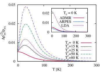
Figure 10: Temperature dependence of the intra-layer magnetoresistance $\Delta\rho_{xx}^{(2)}/\rho_{xx}$ for various $T_{c}$ (or strength of anisotropic scattering) calculated with the AMFL model for the ADMR Fermi surface and for $B_{z}=10$ T. Temperature dependence of the result for $T_{c}=0$ resembles the $T$ dependence of the isotropic scattering, while the anisotropy induces the variation from this result with similar $T$ dependence as observed in $R_{H}$ (see Fig. 8). The magnetoresistance strongly depends on the Fermi surface shape (see inset and Fig. 5). All results are calculated for the fixed chemical potential.

Comparison of our calculations with experimental data for $T_{c}=25$ K (Ref. hussey96, ) is shown in Fig. 11. The calculated magnetoresistance is in qualitative agreement with the experimental data. Use of the LDA Fermi surface give quantitative agreement. However, considering the strong sensitivity of the magnetoresistance to the small changes in the scattering anisotropy zheleznyak99 or of the Fermi surface shape the comparison is good. Previously it was pointed out that the cold spot model ioffe98 cannot describe the intra-layer magnetoresistance of underdoped and optimally doped cuprates. While our model is applicable to the overdoped regime, it cannot describe the optimally doped or underdoped regime, as already mentioned in III.1, presumably due to the emergence of the pseudogap or other new physics not included in our model.

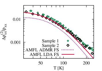
Figure 11: Comparison between the measured intra-layer magnetoresistance $\Delta\rho_{xx}^{(2)}/\rho_{xx}$ at $B_{z}=10$ T for two samples hussey96 and the result of the AMFL model for $T_{c}=25$ K. AMFL results are calculated for the ADMR and LDA Fermi surfaces and agree qualitatively with the measured data.

V.1 Modified Kohler’s rule

It has been observed that in underdoped and optimally doped cuprates Kohler’s rule mckenzie98a , which states that the $\Delta\rho_{xx}^{(2)}/\rho_{xx}$ is a function of $B/\rho_{xx}$, is strongly violated harris95 and therefore two different scattering rates or anisotropic scattering needs to be introduced. Furthermore, it has been realized that $(\Delta\rho_{xx}^{(2)}/\rho_{xx})\cot^{2}\theta_{H}$ is fairly constant with temperature harris95 (modified Kohler’s rule), which was argued harris95 to support the separation of lifetimes picture put forward by Anderson and co-workers, while the anisotropic scattering is inadequate and predicts too large magnetoresistance ioffe98 ; sandeman01 (at least for optimal doping). In Fig. 12 we show AMFL results for $(\Delta\rho_{xx}^{(2)}/\rho_{xx})\cot^{2}\theta_{H}$, which show only weak $T$ dependence for $T>100$ K in the strongly overdoped regime in agreement with experiment. This supports the claims zheleznyak99 ; hussey03a that anisotropic scattering can describe the weak $T$ dependence of this ratio. However, the extent of the $T$ dependence seems to depend strongly on the shape of the Fermi surface and is smaller for more square-like Fermi surfaces. For example, we obtain quantitative agreement with experimental data, if we use the LDA Fermi surface (see inset in Fig. 12). Support for the modified Kohler’s rule can be found also in the approximate $T^{2}$ dependence of $(\Delta\rho_{xx}^{(2)}/\rho_{xx})^{-1/2}$ which is shown in Appendix E.

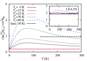
Figure 12: Plot to test modified Kohler’s rule. Temperature dependence of $(\Delta\rho_{xx}^{(2)}/\rho_{xx})\cot^{2}\theta_{H}$, calculated for the AMFL model, is shown for various $T_{c}$. Results show weak $T$ dependence, which is in agreement with the experimental observations shown with dash-dotted black line (ratio $\sim 1.9$) tyler98 . Results were calculated with the ADMR Fermi surface and depend strongly on the shape of the Fermi surface. In the inset we show results for the LDA Fermi surface, which show weaker variation with $T$ and agree quantitatively with experimental data.

VI Comparison with microscopic models

It is a challenge for microscopic theory to quantitatively describe the observed temperature and doping dependence of transport properties or equivalently the proper $T$, $p$ and $\phi$ dependence of the self-energy in the overdoped cuprates. In this section we compare our model self-energy to results from several microscopic theories in order to evaluate their potential for a successful description of the various experimental data.

A weak coupling treatment of the Hubbard model can produce an anisotropic scattering rate of similar frequency and angular dependence to our model. The anisotropic MFL component arises from a nesting of the Fermi surface in the anti-nodal regions roldan06 or from proximity to a van Hove singularity roldan06 ; kastrinakis05 . However, for the latter case the resulting scattering rate would have the opposite doping dependence and would appear only at a higher temperature than that experimentally observed for Tl2201, since the van Hove singularity would reach the Fermi surface for dopings larger than in the highly overdoped regime. Hence, the anisotropic MFL term can only arise from the nested parts of the Fermi surface which produce a particle-hole susceptibility similar to that found in one dimension. Hence, the scattering is essentially arising from particle-hole excitations with a high-frequency cutoff of the order of the band width.

A functional renormalization group treatment of the Hubbard model ossadnik08 (for a review see Ref. rice12, ) shows a $T$, $p$ and $\phi$ dependence of the scattering rate in qualitative agreement with ADMR abdel06 ; abdel07 and our self-energy model. However, it predicts an order of magnitude smaller anisotropic scattering rate than observed in experiment, while it gives the correct order of magnitude for the isotropic scattering ($\propto T^{2}$) in agreement with our self-energy model (see supplemental material of Ref. kokalj11, ).

The Hidden Fermi liquid (HFL) theory by Casey and Anderson anderson06 ; casey11 uses a Gutzwiller projection of the Fermi liquid wave function. However the scattering rate predicted by HFL has a linear $T$ dependence only for temperatures above $T\sim 400$ K, in strong contrast to the ADMR measurements abdel06 , where the $T$ linear term is observed even for $T<60$ K kokalj11 . Furthermore, within the HFL theory the anisotropic scattering emerges solely as a consequence of anisotropy of the Fermi momentum and of the Fermi velocity on the Fermi surface casey ; casey11 . LDA calculations peets07 show a weaker anisotropy and with the opposite doping dependence than that needed in HFL to capture the experimentally observed scattering rates kokalj11 .

Cluster dynamical mean field theory (CDMFT) can also calculate scattering rates at different parts of the Fermi surface. Results presented in Ref. gull10, and obtained with a Hubbard model with $t^{\prime}/t=-0.15$ and $U=7t$ reveal qualitatively similar behaviour to ADMR and to our model self-energy. For higher dopings CDMFT gives an isotropic scattering rate, which becomes more anisotropic (stronger scattering in antinodal direction) and stronger with decreasing doping. However, due to limitations of the quantum Monte Carlo method CDMFT is currently limited to $T>0.05t\sim 200$ K, which is above the most interesting experimental regime. Quantitative comparison with our self-energy model shows, that CDMFT gull10 predicts at $T=200$ K a smaller isotropic part, by a factor $\sim 2.5$. Comparison of the anisotropic part is complicated due to patch averaging in DMFT. However, the CDMFT self-energy gull10 has the same order of magnitude as our model self-energy, at least at $T\sim 200$ K. Detailed quantitative comparison with the CDMFT results is given in Appendix D.

Treatment of the $t$-$J$ model with the finite-temperature Lanczos method (FTLM) jaklic00 yield results in good agreement with several experimental data, including the optical conductivity and high $T$ resistivity. However, the temperature range of reliable results (due to finite size effects) obtained with FTLM is too high to address the low $T$ transport properties and in particular the anisotropy in the scattering rate observed in ADMR.

A large-$N$ expansion treatment of the $t$-$J$ model buzon10 , found a scattering rate with a similar temperature and angular dependence as our model self-energy. However, as optimal doping is approached it also exhibits divergence of the anisotropic scattering rate at low temperature, due to a $d$-density wave instability near optimal doping. This is qualitatively different from our model self-energy.

Ioffe and Millis ioffe98 considered how superconducting fluctuations could produce an anisotropic scattering rate. They suggested that in the overdoped region the rate should scale with $T^{2}$, but it should be kept in mind this depends on what assumptions one makes about the temperature dependence and magnitude of the superconducting correlation length. Superconducting fluctuations used by Ioffe and Millis ioffe98 produce predominantly forward scattering and so it is not clear to what extent they are effective in transport.

Metzner and colleagues have been investigating d-density wave fluctuations near a quantum critical point associated with a Pomeranchuk instability.dellanna07 Their starting point was an effective Hamiltonian which has a d-wave form factor built into it. But this was motivated by earlier work Halboth00 on the Hubbard model which found from renormalisation group flows that strong forward scattering developed led to a Pomeranchuk instability. Although, this work reported an anisotropic scattering rate that is linear in temperature it turns out that due to vertex corrections the transport scattering time scales as $T^{4/3}$ and the resistivity scales as $T^{5/3}$ (Ref. dellanna09, ).

In spite of all these theoretical studies the question remains whether there is a simple explanation for the scattering in terms of a single mechanism: e.g., antiferromagnetic, superconducting, or d-density wave fluctuations. Furthermore, is there a smoking gun experiment which could distinguish between these different contributions? For example, they should have a different dependence on the magnitude of an external magnetic field. We also note that a magnetic field couples differently to spin and orbital degrees of freedom, and the former contribution is dominant for fields parallel to the layers.

VII Conclusions

In conclusion, we have shown that our model self-energy can describe a wide range of experimental data on overdoped cuprates. In earlier work we showed it could describe scattering rates deduced from ADMR, the quasi-particle dispersion seen in ARPES, and effective masses deduced from specific heat and quantum magnetic oscillations kokalj11 . Here, we have shown that neglecting vertex corrections the model can also describe experimental data on electrical transport properties, including DC conductivity, optical conductivity, Hall coefficient, and Hall angle.

The small quantitative discrepancies between the model and measured data at high frequencies ($>$1000 cm^-1) or higher $T$ ($>$300 K) could be reduced with application of a smoother high-frequency cutoff for the self-energy, e.g. with the “parallel resistor” formula hussey03a ; hussey06 .

The successful description of the experimental data by our analysis shows that inclusion of vertex corrections is not necessary at this level of approximation. However, for the Hubbard model on a square lattice it is claimed bergeron11 ; kontani08 that vertex corrections are important in the optimal and underdoped regimes.

Our results on the DC resistivity show that in the overdoped regime the isotropic scattering weakly depends on doping (or $T_{c}$), while the anisotropic scattering increases super-linearly with increasing $T_{c}$ of decreasing doping. Similar findings were obtained for LSCO in Ref. cooper09, . This highlights the fact that the doping dependence of the DC resistivity in cuprates is generic and not so dependent on material properties or Fermi-surface shape.

Such generic behaviour is not seen in the Hall effect, where for overdoped LSCO the Hall coefficient monotonically decreases with increasing temperature and increasing doping narduzzo08 , with a sign change for a doping $p\simeq 0.3$. This may be due to the proximity of the Fermi energy to the van Hove singularity in LSCO.

We have also shown that the main temperature dependence of the Hall coefficient $R_{H}$ comes from the temperature dependence of the self-energy anisotropy. Our model was contrasted with the Marginal Fermi liquid (MFL) model of Abrahams and Varma abrahams03 , which consists of an anisotropic impurity scattering term and an isotropic marginal Fermi liquid term. This model was used to describe the $T$ dependence of the Hall angle at optimal doping. However, their model cannot describe the pronounced non-monotonic $T$ dependence of $R_{H}$ found in overdoped Tl2201. It may be worth noting, that overdoped LSCO, in contrast to Tl2201, shows a monotonic $T$ dependence of $R_{H}$ and so may be adequately described by the MFL model abrahams03 .

On the other hand, the observed $T^{n}$ dependence with $n\lesssim 2$ of $\cot\theta_{H}$ is generic in the cuprates and has in combination with the $T$-linear resistivity stimulated the proposal of more involved theories. For example Anderson anderson91 suggested two types of quasi-particles with different scattering rates. It was suggested that, different scattering mechanism may be connected to the charge conjugation properties of different currentscoleman96 . However, our analysis shows, that there is no need to evoke such theories, since our anisotropic self-energy gives consistent quantitative description of both $\rho_{xx}$ and $\cot\theta_{H}$. In addition, we have shown that it also quantitatively describes the frequency dependent conductivity, remarkably with no additional fitting parameters and just using the parameters originally extracted from ADMR kokalj11 .

Future work would could and should consider calculation of thermoelectric transport properties such as the Seebeck coefficient and Nernst signal using the same model self-energy. In a quasi-particle picture both of these transport coefficients contain contributions from the energy dependence of the scattering time behnia04 ; behnia09 and so may be sensitive to a marginal Fermi liquid contribution to the self-energy.

The relevance of the model self-energy to electron doped cuprates Armitage10 should also be investigated. Recently it was observed Jin11 that in the overdoped region of the phase diagram the resistivity had a linear-in-temperature term which was proportional to the superconducting $T_{c}$, as in the hole doped cuprates considered here.

The broader significance of this work is that it shows that the metallic state in the overdoped regime is not a simple Fermi liquid and exhibits some physics which is similar to that found at optimal doping [marginal Fermi liquid behaviour] and underdoping [anisotropic Fermi surface properties with cold spots in the nodal directions]. A significant challenge is to find a general phenomenological form of the self-energy that with decreasing doping smoothly crosses over to a form that describes the pseudogap state, such as the form proposed by Yang, Zhang, and Rice yang06 ; rice12 .

Appendix A Functions $f_{H}(\phi)$ and $f_{DC}(\phi)$

Here we give explicit forms for the functions $f_{H}(\phi)$ and $f_{DC}(\phi)$ that appear in Eq. (31). The function $f_{H}(\phi)$ can be readily obtained from Eq. (24) for $\sigma_{xy}^{(1)}$,

$$f_{H}(\phi)=\frac{e^{3}}{4\pi^{2}d}(-{\bf v}_{0,F}(\phi)\times\partial_{\phi}{\bf v}_{0,F}(\phi))_{z}.$$ (37)

On the other hand, $f_{DC}(\phi)$ can be obtained from Eq. (17) for ${\rm Re}\ \sigma_{xx}$,

$$f_{DC}(\phi)=\frac{e^{2}}{4\pi^{2}d}\frac{k_{F}(\phi)v_{0,F}^{2}(\phi)}{v_{0,F,r}(\phi)}.$$ (38)

Appendix B Details on derivation of Hall conductivity

Here we give more details of the derivation of the expression for the Hall conductivity, Eq. (24), by starting with Eq. (23), which is taken from Eqs. (2.7) and (3.36) in Ref. kohno88, . $J_{x}$ in Eq. (23) represents the current vertex, which in our approximation of neglecting vertex corrections equals $-ev_{x}$. The square brackets denote

$$[A\tilde{\partial}_{\mu}B]=A\partial_{k_{\mu}}B-(\partial_{k_{\mu}}A)B,$$ (39)

which leads to

$$[J_{x}\tilde{\partial}_{y}J_{y}]=e^{2}(v_{x}\partial_{k_{y}}v_{y}-v_{y}\partial_{k_{y}}v_{x}),$$ (40)

$$[G^{R}\tilde{\partial}_{x}G^{A}] = G^{R}\partial_{k_{x}}G^{A}-\partial_{k_{x}}(G^{R})G^{A}$$ (41)

$$= G^{R}G^{A}(G^{A}(\hbar v_{x}+\partial_{k_{x}}\Sigma^{A})$$

$$-G^{R}(\hbar v_{x}+\partial_{k_{x}}\Sigma^{R})).$$

$G^{R(A)}$ represent the retarded (advanced) Green’s function, which may be written in terms of retarded (advanced) self-energy $\Sigma^{R(A)}$. With the use of $\Sigma^{R}=\Sigma^{A*}=\Sigma=\Sigma^{\prime}+{\rm i}\Sigma^{\prime\prime}$ and $G^{R(A)}=1/(\omega-\epsilon_{k}-\Sigma^{R(A)})$ we can write

$$[G^{R}\tilde{\partial}_{x}G^{A}]=\frac{1}{[(\omega-\epsilon_{k}-\Sigma^{\prime})^{2}+(\Sigma^{\prime\prime})^{2}]^{2}}$$ (42)

$$\times\big{[}(\hbar v_{x}+\partial_{k_{x}}\Sigma^{\prime})(-2{\rm i}\Sigma^{\prime\prime})+(-2{\rm i}\partial_{k_{x}}\Sigma^{\prime\prime})(\omega-\epsilon_{k}-\Sigma^{\prime})\big{]}.$$

The Hall conductivity can now be written as

$$\sigma_{xy}^{(1)}=\frac{-{\rm i}e^{3}B_{z}}{2}\sum_{k}\int\frac{d\omega}{2\pi}(-\frac{\partial n_{F}(\omega)}{\partial\omega})$$ (43)

$$\times(v_{x}\partial_{k_{y}}v_{y}-v_{y}\partial_{k_{y}}v_{x})\frac{1}{[(\omega-\epsilon_{k}-\Sigma^{\prime})^{2}+(\Sigma^{\prime\prime})^{2}]^{2}}$$

$$\times\big{[}(v_{x}+\partial_{k_{x}}\Sigma^{\prime})(-2{\rm i}\Sigma^{\prime\prime})+(-2{\rm i}\partial_{k_{x}}\Sigma^{\prime\prime})(\omega-\epsilon_{k}-\Sigma^{\prime})\big{]}.$$

Since we neglected vertex corrections we should also neglect $\partial_{k_{x}}\Sigma^{\prime}$ in the above equation, which is the same as neglecting the first correction to the vertex. For our even-in-$\omega$ $\Sigma^{\prime\prime}$ first order vertex corrections ($v_{x}\to v_{x}+\partial_{k_{x}}\Sigma^{\prime}$) turn out to be negligible. Also the term with $(\omega-\epsilon_{k}-\Sigma^{\prime})$ may be neglected due to the strongly peaked and even-in-$\omega$ prefactor $1/[(\omega-\epsilon_{k}-\Sigma^{\prime})^{2}+(\Sigma^{\prime\prime})^{2}]^{2}$.

$$\sigma_{xy}^{(1)} = \frac{e^{3}B_{z}}{2}\sum_{k}\int\frac{d\omega}{2\pi}(-\frac{\partial n_{F}(\omega)}{\partial\omega})$$ (44)

$$\times\tilde{v}(k)\frac{-2\Sigma^{\prime\prime}}{[(\omega-\epsilon_{k}-\Sigma^{\prime})^{2}+(\Sigma^{\prime\prime})^{2}]^{2}},$$

where

$$\tilde{v}(k)=v_{x}^{2}\partial_{k_{y}}v_{y}-v_{x}v_{y}\partial_{k_{y}}v_{x}.$$ (45)

The sum over $k$ may be converted to an integral over the first BZ, and the integral over $k_{z}$ can be performed due to the quasi-two-dimensional nature of the system. The integral over $k_{x}$ and $k_{y}$ may be decomposed into integrals over $k_{r}$ [the radial direction from $(\pi,\pi)$, see Fig. 5] and its azimuthal angle $\phi$. We are left with

$$\sigma_{xy}^{(1)} = \frac{e^{3}B_{z}}{(2\pi)^{3}d}\int d\phi\int d\omega(-\frac{\partial n_{F}(\omega)}{\partial\omega})$$ (46)

$$\times\int dk_{r}k_{r}\hat{v}(k)\frac{-2\Sigma^{\prime\prime}}{[(\omega-\epsilon_{k}-\Sigma^{\prime})^{2}+(\Sigma^{\prime\prime})^{2}]^{2}}.$$

In the next step we linearize the bare band dispersion close to the Fermi surface in the $k_{r}$ direction [see Eq. (8)] and approximate

$$\frac{1}{[(\omega-\epsilon_{k}-\Sigma^{\prime})^{2}+(\Sigma^{\prime\prime})^{2}]^{2}}\simeq$$

$$\frac{\pi}{2(-\Sigma^{\prime\prime}(\phi,\omega))^{3}v_{0,F,r}(\phi)}\delta[k_{r}-\tilde{k}_{r}(\phi,\omega)],$$ (47)

with

$$\tilde{k}_{r}(\phi,\omega)=k_{F}(\phi)+\frac{\omega-\Sigma^{\prime}(\phi,\omega)}{v_{0,F,r}(\phi)}.$$ (48)

We further approximate $\tilde{k}_{r}(\phi,\omega)\sim k_{F}(\phi)$, which we have checked numerically results in an error of less than 2% for the relevant band structures. With this approximation the integral over $k_{r}$ can be explicitly evaluated.

$$\sigma_{xy}^{(1)}=\frac{e^{3}B_{z}}{2\pi^{2}d}\int d\phi\frac{k_{F}(\phi)\hat{v}(k_{F}(\phi),\phi)}{v_{0,F,r}(\phi)}$$

$$\times\int d\omega(-\frac{\partial n_{F}(\omega)}{\partial\omega})\frac{1}{(-2\Sigma^{\prime\prime}(\phi,\omega))^{2}}.$$ (49)

There is one further simplification regarding the ”velocity” term that can be done. Using the symmetry $\sigma_{xy}^{(1)}=-\sigma_{yx}^{(1)}$ we can write Eq. (45)

$$\tilde{v} \to \frac{1}{2}[v_{x}^{2}\partial_{k_{y}}v_{y}+v_{y}^{2}\partial_{k_{x}}v_{x}-v_{y}v_{x}(\partial_{k_{y}}(v_{x})+\partial_{k_{x}}(v_{y}))]$$ (50)

$$= \frac{1}{2}({\bf v}\times{\bf e}_{z})\cdot(v_{y}{\bf\nabla}v_{x}-v_{x}{\bf\nabla}v_{y}).$$

Expressing $({\bf v}\times{\bf e_{z}})=v{\bf t}$, where ${\bf t}$ is unit vector parallel to the Fermi surface, and using

$${\bf\nabla}v_{x}\cdot{\bf t}=\frac{{\bf\nabla}v_{x}\cdot{\bf t}dk_{\parallel}}{dk_{\parallel}}=\frac{\partial_{\phi}v_{x}(\phi)}{k_{f}(\phi)/\cos\theta},$$ (51)

where $\theta$ is the angle between the Fermi surface direction and direction ${\bf e}_{\phi}$ (perpendicular to $k_{r}$). Analysing in the same way the $y$ term brings us to

$$\tilde{v}\to\frac{1}{2}v_{0,F}(\phi)[-{\bf v}_{0,F}\times\partial_{\phi}{\bf v}_{0,F}(\phi)]_{z}\frac{\cos\theta}{k_{F}(\phi)}.$$ (52)

Finally, using $v_{0,F,r}(\phi)=\cos\theta v_{0,F}(\phi)$ cancels $\cos\theta$ and we can write our result as Eq. (24).

Appendix C Effect of anisotropy on Hall effect

Here we demonstrate how the anisotropy in the scattering rate influences the Hall effect. In particular, we show with a simple example that the $T$-dependence of the Hall coefficient $R_{H}$ is dominated by $T$-dependent anisotropy, while, on the other hand, the Hall angle $\cot\theta_{H}$ and its $T$-dependence are dominated by the isotropic scattering. We start with the expressions for conductivities, which were used in obtaining Eq. (31),

$$\sigma_{xx}=\int d\phi f_{DC}(\phi)\frac{1}{-2\Sigma^{\prime\prime}(\phi,0)},$$ (53)

$$\sigma_{xy}=\int d\phi f_{H}(\phi)\frac{1}{(-2\Sigma^{\prime\prime}(\phi,0))^{2}}.$$ (54)

In this simple approximation we neglect the $\phi$ dependence of functions $f_{H}(\phi)$ and $f_{DC}(\phi)$ and exchange them with their average values $\bar{f}_{H}$ and $\bar{f}_{DC}$. This is feasible due to the much stronger anisotropy in the self-energy than in the $f$-functions. Further on, we use a shorter notation for the two self-energy parts, $-\Sigma^{\prime\prime}_{\textrm{FL}}(0)=a$ and $-\Sigma_{\textrm{AMFL}}(0,0)=b$, which allows us to write

$$-\Sigma^{\prime\prime}(\phi,0)=a+b\cos^{2}(2\phi),$$ (55)

where $a$ and $b$ are $T$ dependent. $a$ includes impurity scattering and the FL like part which is $\propto T^{2}$, while $b$ is due to the AMFL part and is $\propto T$. With this approximation, integrals over $\phi$ in Eq. (53) and (54) can be explicitly performed and lead to

$$\sigma_{xx}=\pi\bar{f}_{DC}\frac{1}{a(1+\frac{b}{a})^{1/2}},$$ (56)

$$\sigma_{xy}=\frac{\pi}{4}\bar{f}_{H}\frac{2+\frac{b}{a}}{a^{2}(1+\frac{b}{a})^{3/2}}.$$ (57)

Expressing the Hall coefficient and Hall angle in this approximation brings us to the final result of this section,

$$R_{H}=\frac{1}{4\pi}\frac{\bar{f}_{H}}{\bar{f}_{DC}^{2}}\sqrt{1+\frac{b}{a}}(1+\frac{1}{1+b/a}),$$ (58)

$$\cot\theta_{H}=4\frac{\bar{f}_{DC}}{\bar{f}_{H}}a(1+\frac{1}{1+b/a})^{-1}.$$ (59)

From Eq. (58) it is evident that the Hall coefficient, and in particular its $T$ dependence, are dominated by the $T$-dependent anisotropy $b/a$. On the other hand, Eq. (59) reveals that the Hall angle $\cot\theta_{H}$ is dominated by the isotropic scattering $a$, while the anisotropy effect is strongly suppressed in the factor $(1+\frac{1}{1+b/a})^{-1}$. The doping and $T$ dependence of $(1+\frac{1}{1+b/a})^{-1}$ for our model self-energy are shown in Fig. 13. The effect of anisotropy can be further increased or decreased by $\phi$ dependent $f_{H}$ or $f_{DC}$, which can either increase or decrease the contribution from the AMFL part of the self-energy (or the antinodal part of the Fermi surface). The effect of changing the $f$-functions by changing the shape of the Fermi surface can for example be seen in Fig. 6. Furthermore, the effect of the anisotropy factor $(1+\frac{1}{1+b/a})^{-1}$ is to downturn the $T^{2}$ dependence of $\cot\theta_{H}$ and make it more like $T^{n}$ with $n\leq 2$, which has in fact been observed (see inset in Fig. 9 and Refs. ando99, ; fruchter07, .)

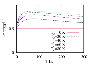
Figure 13: Small temperature dependence of the factor $(1+\frac{1}{1+b/a})^{-1}$ appearing in $\cot\theta_{H}$. This factor shows less than 10% variation with $T$ from 50 to 300 K. Therefore the main $T$ dependence of $\cot\theta_{H}$ comes from the isotropic scattering, which in our model self-energy is $\propto T^{2}$ (in agreement with experiment).

Appendix D Comparison of model self-energy with CDMFT

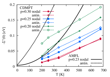
Figure 14: Comparison of the imaginary part of the self-energy at zero frequency ($-\Sigma"(\omega=0)$) from CDMFT results (Ref. gull10, Fig. 11) with our model self-energy. CDMFT results were obtained for different doping levels $p=0.3,0.25,$ and $0.2$ and for different patches on the Fermi surface (“nodal” denotes nodal patch, while “antin.” denotes antinodal patch). CDMFT results are only available at higher temperatures ($T>200K$) due to limitations of the quantum Monte Carlo method used. Our model self-energy is most reliable at low $T$. (Experiments suggest it should become more linear for $T>200$ K (see Fig. 2)). Most reliable comparison with CDMFT can therefore be done at $T=200$ K. At such $T$ CDMFT predicts a weaker isotropic self-energy (compare CDMFT $n=0.70$ and our nodal self-energy). Quantitative comparison for stronger anisotropies or lower doping is more difficult due to patch averaging in CDMFT. However, CDMFT predicts the correct trend with doping and order of the magnitude for the self-energy. Our antinodal self-energy was calculated with $T_{c}=60$ K, and the energy scale of CDMFT data was set with the hopping parameter $t_{1}=0.438$ eV.

Here we show a quantitative comparison of our model self-energy with Cluster Dynamical Mean-Field Theory (CDMFT) calculations on the Hubbard model gull10 . Scattering at the Fermi surface or $\Sigma^{\prime\prime}(\omega=0)$ is the most relevant quantity for explanation of many transport data, which we analyze in this work. Our model $\Sigma^{\prime\prime}(\omega=0)$ at a doping level $p=0.3$ is compared with CDMFT results in Fig. 14. Comparison of the dependence of the self-energy on the Matsubara frequencies on imaginary axis (see Fig. 15) can be done to avoid analytical continuation of CDMFT results. The slope at low frequencies ($\partial_{\omega_{n}}{\rm Im}\Sigma(i\omega_{n})|_{\omega_{n}\to 0}$) is related to the quasi-particle weight and mass renormalisation.

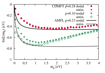
Figure 15: Comparison of results for the Matsubara frequency dependence of ${\rm Im}\Sigma(i\omega_{n})$ from CDMFT (Ref. gull10, Fig. 8) with our model self-energy. It is seen that the saturated value of the self-energy is similar in both results. The isotopic CDMFT result ($p=0.28$) predicts a smaller slope at low frequencies (and thus are a quasi-particle weight closer to one) than our model. Parameters for our model self-energy are the same as in Fig. 14 and the temperature corresponds to that of the CDMFT calculation, $T=0.05t_{1}\sim 250K$.

Appendix E Temperature dependence of intra-layer magnetoresistance

Intra-layer magnetoresistance $\Delta\rho^{(2)}_{xx}/\rho_{xx}$ shows similarly to $\cot\theta_{H}$ (Fig. 9) $T^{2}$ temperature dependence, at least at higher $T$. This is shown in Fig. 16 and implies the behaviour according to the modified Kohler’s rule.

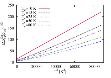
Figure 16: Inverse square root of the intra-layer magnetoresistance, $(\Delta\rho_{xx}^{(2)}/\rho_{x}x)^{-1/2}$ vs. $T^{2}$. With this choice of the axes the $T^{2}$ behaviour of $(\Delta\rho_{xx}^{(2)}/\rho_{x}x)^{-1/2}$ becomes more apparent (at least at high $T$) and shows similar behaviour to $\cot\theta_{H}$. Therefore the ratio of the two is expected to show weak $T$ dependence and obeys the modified Kohler’s rule as already discussed in the main text and shown in Fig. 12. Curves are calculated with the ADMR Fermi surface and for several $T_{c}$s.

References

- (1) A. Damascelli, Z. Hussain, Z.X. Shen, Rev. Mod. Phys. 75, 473 (2003).
- (2) T. Valla, A.V. Fedorov, P.D. Johnson, B.O. Wells et al., Science 285, 2110 (1999).
- (3) T. Valla, A.V. Fedorov, P.D. Johnson, Q. Li et al., Phys. Rev. Lett. 85, 828 (2000).
- (4) A.A. Kordyuk, S.V. Borisenko, A. Koitzsch, J. Fink et al., Phys. Rev. Lett. 92, 257006 (2004).
- (5) A. Kaminski, H.M. Fretwell, M.R. Norman, M. Randeria et al., Phys. Rev. B 71, 014517 (2005).
- (6) J. Chang, M. Shi, S. Pailhés, M. Månsson et al., Phys. Rev. B 78, 205103 (2008).
- (7) L. Zhu, V. Aji, A. Shekhter, C.M. Varma, Phys. Rev. Lett. 100, 057001 (2008).
- (8) M. Platé, J.D.F. Mottershead, I.S. Elfimov, D.C. Peets et al., Phys. Rev. Lett. 95, 077001 (2005).
- (9) J.M. Wade, J.W. Loram, K.A. Mirza, J.R. Cooper et al., J. Supercond. 7, 261 (1994).
- (10) J.W. Loram, K.A. Mirza, J.M. Wade, J.R. Cooper et al., Physica C 235-240, 134 (1994).
- (11) M. Abdel-Jawad, M.P. Kennett, L. Balicas, A. Carrington et al., Nature Phys. 2, 821 (2006).
- (12) M. Abdel-Jawad, J.G. Analytis, L. Balicas, A. Carrington et al., Phys. Rev. Lett. 99, 107002 (2007).
- (13) J.G. Analytis, M. Abdel-Jawad, L. Balicas, M.M.J. French et al., Phys. Rev. B 76, 104523 (2007).
- (14) M.P. Kennett, R.H. McKenzie, Phys. Rev. B 76, 054515 (2007).
- (15) A.W. Tyler (Ph. D. thesis, University of Cambridge, 1997).
- (16) A.W. Tyler, Y. Ando, F.F. Balakirev, A. Passner et al., Phys. Rev. B 57, R728 (1998).
- (17) T. Manako, Y. Kubo, Y. Shimakawa, Phys. Rev. B 46, 11019 (1992).
- (18) A.P. Mackenzie, S.R. Julian, D.C. Sinclair, C.T. Lin, Phys. Rev. B 53, 5848 (1996).
- (19) N.E. Hussey, J. Phys.: Condens. Matter 20, 123201 (2008).
- (20) N.E. Hussey, J.R. Cooper, J.M. Wheatley, I.R. Fisher et al., Phys. Rev. Lett. 76, 122 (1996).
- (21) Y. Kubo, Y. Shimakawa, T. Manako, H. Igarashi, Phys. Rev. B 43, 7875 (1991).
- (22) D.N. Basov, T. Timusk, Rev. Mod. Phys. 77, 721 (2005).
- (23) A.V. Puchkov, D.N. Basov, T. Timusk, J. Phys.: Condens. Matter 8, 10049 (1996).
- (24) Y.C. Ma, N.L. Wang, Phys. Rev. B 73, 144503 (2006).
- (25) D.N. Basov, R.D. Averitt, D. van der Marel, M. Dressel et al., Rev. Mod. Phys. 83, 471 (2011).
- (26) J. Kokalj, R.H. McKenzie, Phys. Rev. Lett. 107, 147001 (2011).
- (27) P.M.C. Rourke, A.F. Bangura, T.M. Benseman, M. Matusiak et al., New J. Phys. 12, 105009 (2010).
- (28) E. Abrahams, C.M. Varma, Phys. Rev. B 68, 094502 (2003).
- (29) C.M. Varma, P.B. Littlewood, S. Schmitt-Rink, E. Abrahams et al., Phys. Rev. Lett. 63, 1996 (1989).
- (30) P.B. Littlewood, C.M. Varma, J. Appl. Phys. 69, 4979 (1991).
- (31) C. Varma, Z. Nussinov, W. van Saarloos, Physics Reports 361, 267 (2002).
- (32) A.C. Jacko, J.O. Fjærestad, B.J. Powell, Nature Phys. 5, 422 (2009).
- (33) J.L. Tallon, C. Bernhard, H. Shaked, R.L. Hitterman et al., Phys. Rev. B 51, 12911 (1995).
- (34) A.F. Bangura, P.M.C. Rourke, T.M. Benseman, M. Matusiak et al., Phys. Rev. B 82, 140501 (2010).
- (35) M.M.J. French, J.G. Analytis, A. Carrington, L. Balicas et al., New J. Phys. 11, 055057 (2009).
- (36) Y.M. Vilk, A.-M.S. Tremblay, J. Phys. I France 7, 1309 (1997).
- (37) D.C. Peets, J.D.F. Mottershead, B. Wu, I.S. Elfimov et al., New J. Phys. 9, 28 (2007).
- (38) H. Bruus, K. Flensberg, Many-Body Quantum Theory in Condensed Matter Physics: An Introduction (Oxford University Press, USA, 2004), p. 37.
- (39) N.W. Ashcroft, N.D. Mermin, Solid State Physics, 1st edn. (Thomson Learning, Toronto, 1976), p. 252, Eq. 13.36.
- (40) R.A. Cooper, Y. Wang, B. Vignolle, O.J. Lipscombe et al., Science 323, 603 (2009).
- (41) N.E. Hussey, Eur. Phys. J. B 31, 495 (2003).
- (42) O. Gunnarsson, M. Calandra, J.E. Han, Rev. Mod. Phys. 75, 1085 (2003).
- (43) M. Dressel, G. Gruner, Electrodynamics of Solids (Optical properties of electrons in matter) (Cambrige University Press, 2002), p. 37.
- (44) N.E. Hussey, J.C. Alexander, R.A. Cooper, Phys. Rev. B 74, 214508 (2006).
- (45) M.R. Norman, A.V. Chubukov, Phys. Rev. B 73, 140501 (2006).
- (46) H. Kohno, K. Yamada, Progress Theor. Phys. 80, 623 (1988).
- (47) N.P. Ong, Phys. Rev. B 43, 193 (1991).
- (48) B.P. Stojković, D. Pines, Phys. Rev. B 55, 8576 (1997).
- (49) A. Carrington, A.P. Mackenzie, C.T. Lin, J.R. Cooper, Phys. Rev. Lett. 69, 2855 (1992).
- (50) L.B. Ioffe, A.J. Millis, Phys. Rev. B 58, 11631 (1998).
- (51) L. Fruchter, H. Raffy, F. Bouquet, Z.Z. Li, Phys. Rev. B 75, 092502 (2007).
- (52) H. Castro, G. Deutscher, Phys. Rev. B 70, 174511 (2004).
- (53) Y. Ando, T. Murayama, Phys. Rev. B 60, R6991 (1999).
- (54) P.W. Anderson, Phys. Rev. Lett. 67, 2092 (1991).
- (55) P. Coleman, A.J. Schofield, A.M. Tsvelik, Phys. Rev. Lett. 76, 1324 (1996).
- (56) A.T. Zheleznyak, V.M. Yakovenko, H.D. Drew, Phys. Rev. B 59, 207 (1999).
- (57) K.G. Sandeman, A.J. Schofield, Phys. Rev. B 63, 094510 (2001).
- (58) For a brief review see R.H. McKenzie, J.S. Qualls, S.Y. Han, J.S. Brooks, Phys. Rev. B 57, 11854 (1998).
- (59) J.M. Harris, Y.F. Yan, P. Matl, N.P. Ong et al., Phys. Rev. Lett. 75, 1391 (1995).
- (60) R. Roldán, M.P. López-Sancho, F. Guinea, S.W. Tsai, Phys. Rev. B 74, 235109 (2006).
- (61) G. Kastrinakis, Phys. Rev. B 71, 014520 (2005).
- (62) M. Ossadnik, C. Honerkamp, T.M. Rice, M. Sigrist, Phys. Rev. Lett. 101, 256405 (2008).
- (63) T.M. Rice, K.Y. Yang, F.C. Zhang, Reports on Progress in Physics 75, 016502 (2012).
- (64) P.W. Anderson, Nature Phys. 2, 626 (2006).
- (65) P.A. Casey, P.W. Anderson, Phys. Rev. Lett. 106, 097002 (2011).
- (66) P.A. Casey, Hidden Fermi liquid: self-consistent theory for the normal state of high- superconductors (Ph.D. Dissertation, Princeton University, 2010).
- (67) E. Gull, M. Ferrero, O. Parcollet, A. Georges et al., Phys. Rev. B 82, 155101 (2010).
- (68) J. Jaklič, P. Prelovšek, Adv. Phys. 49, 192 (2000).
- (69) G. Buzon, A. Greco, Phys. Rev. B 82, 054526 (2010).
- (70) L. Dell’Anna, W. Metzner, Phys. Rev. Lett. 98, 136402 (2007).
- (71) C.J. Halboth, W. Metzner, Phys. Rev. Lett. 85, 5162 (2000).
- (72) L. Dell’Anna, W. Metzner, Phys. Rev. Lett. 103, 159904(E) (2009).
- (73) D. Bergeron, V. Hankevych, B. Kyung, A.M.S. Tremblay, Phys. Rev. B 84, 085128 (2011).
- (74) H. Kontani, Rep. Prog. Phys. 71, 026501 (2008).
- (75) A. Narduzzo, G. Albert, M.M.J. French, N. Mangkorntong et al., Phys. Rev. B 77, 220502 (2008).
- (76) K. Behnia, D. Jaccard, J. Flouquet, J. Phys.: Cond. Matter 16, 5187 (2004).
- (77) K. Behnia, J. Phys.: Cond. Matter 21, 113101 (2009).
- (78) N.P. Armitage, P. Fournier, R.L. Greene, Rev. Mod. Phys. 82 (2010).
- (79) K. Jin, N.P. Butch, K. Kirshenbaum, J. Paglione et al., Nature 476, 73 (2011).
- (80) K.Y. Yang, T.M. Rice, F.C. Zhang, Phys. Rev. B 73, 174501 (2006).