QCDUTILS
Abstract
This manual describes a set of utilities developed for Lattice QCD computations. They are collectively called qcdutils. They are comprised of a set of Python programs each of them with a specific function: download gauge ensembles from the public NERSC repository, convert between formats, split files by time-slices, compile and run physics algorithms, generate visualizations in the form of VTK files, convert the visualizations into images, perform bootstrap analysis of results, fit the results of the analysis, and plot those results. These tools implement the typical workflow of most Lattice QCD computations and automate it by enforcing filename conventions: the output of one tool is understood by the next tool in the workflow. This manual is organized as a series of autonomous recipes which can be combined together.
1 Introduction
In this manual we provide a description of the following tools:
- •
-
•
qcdutils_run.py: a program to download, compile and run various parallel Physics algorithms (for example compute the average plaquette, the topological charge density, two and three points correlation functions). qcdutils_run is a proxy for FermiQCD. Most of the FermiQCD algorithms and examples generate files that are suitable for visualization (VTK files [5])
-
•
qcdutils_vis.py: a program to manipulate the VTK files generated by qcdutils_run which can be used to split VTK files into components, interpolate them, and generate 3D contour plots as JPEG images. This program uses metaprogramming to write a VisIt [6] script and runs it in background.
-
•
qcdutils_vtk.py: a program that converts a VTK file into a web page (HTML) which displays iso-surfaces computed from the VTK file. The generated files can be visualized in any browser and allows interactive rotation of the visualization. This program is a based on the “processing.js” library [7].
-
•
qcdutils_boot.py: a tools for performing bootstrap analysis of the output of qcdutils_run and other QCD Software. It computes autocorrelations, moving averages, and distributions.
-
•
qcdutils_plot.py: a tool to plot results from qcdutils_boot.
-
•
qcdutils_fit.py: a tool to fit results from qcdutils_boot.py.
As the .py extension implied, these programs are written in Python [8] (2.7 version recommended).
Together these tools allow automation of the workflow of most Lattice QCD computations from downloading data to computing scientific results, plots, and visualizations.
Notice that each of the utilities has its own help page which you an access using the -h command line option. The output for each is reported in the Appendix.
The data downloaded by qcdutils_get can be read by qcdutils_run which executes the physics algorithms implemented in C++. The output can be VTK files manipulated by qcdutils_vis and and then transformed into images and movies by VisIt, or they can be tabulated data that require bootstrap analysis. This is done by qcdutils_boot. The output of the latter plotted by qcdutils_plot and can be fitted with qcdutils_fit.
These files enforce a workflow by following the file naming conventions described in the Appendix but, they do not strictly depend on each other. For example qcdutils_boot can be used to analyze the output of any of your own physics simulations even if you do not use qcdutils_run.
Here is an overview of the workflow:
This manual is not designed to be complete or exhaustive because our tools are in continuous development and new features are added every day. Yet is designed to provide enough examples to allow you to explore further. Our analysis and visualizations are created on sample data and aimed exclusively at explaining how to use the tools.
Our hope is that these tools will be useful to practitioners in the field and specifically to graduate students new to the field of Lattice QCD and looking to jumpstart their research projects.
These tools can also be used to automate the workflow of analyzing gauge configurations in real time in order to obtain and display preliminary results.
Some of the tools described here find more general application than Lattice QCD and can be utilized in other scientific areas.
1.1 Resources
qcdutils can be downloaded from:
http://code.google.com/p/qcdutils
More information FermiQCD code used by qcdutils_run is available from refs. [3, 4] and the web page:
http://fermiqcd.net
More examples of visualizations and links do additional code and examples can be found at:
http://latticeqcd.org
1.2 Getting the tools
There are two ways to get the tools described in here. The easiest way to get qcdutils is to use Mercurial:
Install mercurial from:
and download qcdutils from the googlecode repository
using the following commands:
The command creates a folder called “qcdutils” and download the latest source files in there.
You can also download individual files using wget (default on Linux systems) or curl (default on mac systems):
1.3 Dependencies
These files do not depend on each other so you can download only those that you need. qcdutils_run is special because it is a Python interface to the FermiQCD library. As it is explained later, when executed, it downloads and compiles FermiQCD. It assumes you have g++ installed.
qcdutils_fit.py and qcdutils_plot.py requires the Python numpy and matplotlib installed.
All the file require Python 2.x (possibly 2.7) and do not work with Python 3.x.
1.4 License
qcdutils are released under the GPLv2 license.
1.5 Acknowledgments
We thank all members of the USQCD collaborations for making most of their their data and code available to the public, and for a long-lasting collaboration. We thank David Skinner, Schreyas Cholia, and Jim Hetrick for their collaboration in improving and running the NERSC gauge connection. We particularly thank Jim Hetrick for sharing his code for t’Hooft instantons. We thank Chris Maynard for useful discussions about ILDG. We thanks Simon Catterall, Yannick Meurice, Jonathan Flynn, and all those that over time have submitted patches for FermiQCD thus contributing to make it better. We also thank all of those who have used and who still use FermiQCD, thus providing the motivation for continuing this work. We thank the graduate students that over time have helped with coding, testing, and documentation: Yaoqian Zhong, Brian Schinazi, Nate Wilson, Vincent Harvey, and Chris Baron.
This work was funded by Department of Energy grant DEFC02-06ER41441 and by National Science Foundation grant 0970137.
2 Accessing public data with qcdutils_get.py
2.1 Searching data on the NERSC Gauge Connection
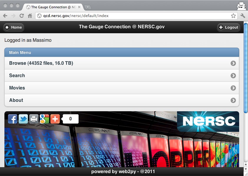
The Gauge Connection [1] is a repository of Lattice QCD data, primarily but not limited to gauge ensembles, hosted by the National Energy Research Science Center (NERSC) on their High Performance Storage System (HPSS). At the time of writing the Gauge Connection hosts 16 Terabytes of data and makes it publicly accessible to researchers worldwide.
The new Gauge Connection site consists of a set of dynamic web pages in hierarchical structures that closely mimics the folder structure in the HPSS FTP server. Each folder corresponds to a web page. The web page provide a description of the folder content, in the form of an editable wiki, comments about the content, links to sub-folder and links to files contained in the folder. Since folders may contain thousands of files, files with similar filenames are grouped together into filename patterns. For example all files with the same name but different extension or similar names differing only for a numerical value are grouped together. Pages are tagged and can be searched by tag. Users can search for files by browsing the folder structure, searching by tags and can download individual files or all files matching a pattern.
You do not need an account to login and you can use your OpenID account, for example a Google email account. You do not need to login to search but you need to login to download. From now on we assume you are logged in into the Gauge Connection.
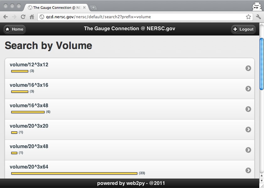
Fig 1 (left) is a screenshot of the main Gauge Connection site. Each gauge ensemble is stored in a folder which is represented by a dynamic web page and tagged. You can search these pages by tag, as shown in Fig. 1 (right).
 |
 |
Fig. 2 (left) shows statistical information about tags.
Each tag has the form “type/value” where the tag type can be:
-
•
source: the name of the organization who donated the data, value can be, for example MILC [9].
-
•
flavor, the flavor content of the data, value can be “0” for quenched data, “2” for two flavor unquenched data, “2+1” for three flavor unquenched where two quarks have one mass and 1 quark has another mass.
-
•
kappa: the value
-
•
mass: the quark mass
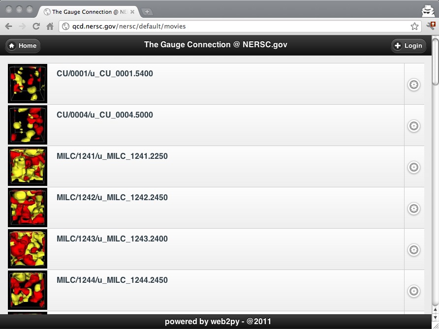
We have also processed many of the ensambes using some of the tools described here and generated animations of the topological charge densities. This is shown in fig. 2 (right).
 |
 |
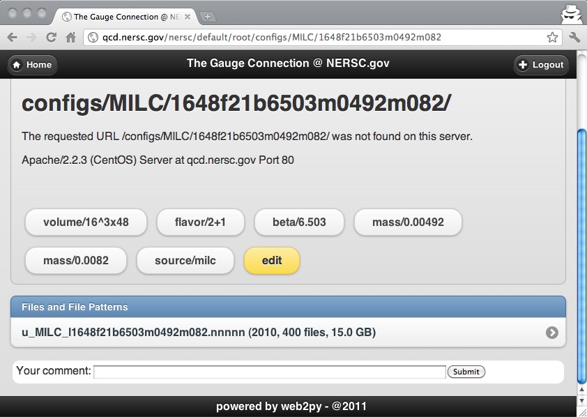
A screenshot of a folder page is shown in fig. 3 (left)
You can see a description, a list of tags, list of file patterns in the folder, and comments. The comments are only visible to logged in users. The login link is at top left of the page.
A screenshot of a page listing the files in an ensemble is shown in fig. 3 (right)
 |
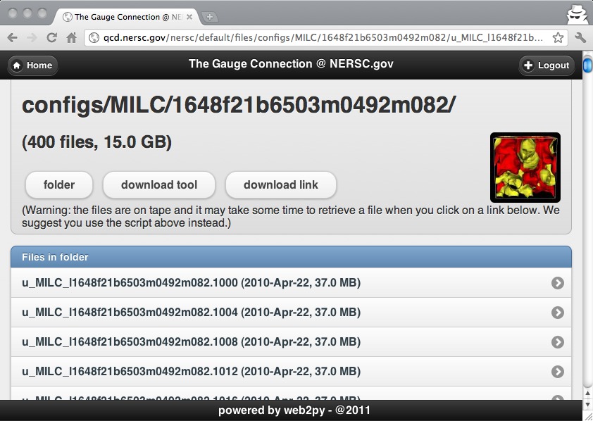 |
You can download an individual files by clicking on the file.
To download files in batch you need to first download qcdutils_get.py. The web page page above includes a link [download tool] that explains where to get and how to use qcdutils_get.py. We suggest you first read the rest of this section but also read the linked instructions which may be more updated. The page also contains a link [download link] which is used to reference the data for later download.
2.2 Downloading data from NERSC
Here we assume you want to download the 400 MILC gauge configurations of size and computed using 2+1 quarks of mass respectively (light) and (heavy). These files can be found at
where you should notice the folder name
It follows the MILC filename convention
and the values of [beta] and [mass] omit the decimal point.
The above page links the pattern page:
where
is the filename pattern and nnnnn is just a wildcard for the gauge configuration numbers in the ensemble.
The page contains a [download link] to a document in JSON format listing all files in the folder matching the pattern and additional meta-data about each file. You do not need to open this document. All you need to do is copy the link address and pass it to qcdutils_get.py as a command line argument. The program opens the URL, download the list, loop over the files in the ensemble, and download them one by one.
Copy the download link to clipboard and it looks something like this:
We have shortened the full actual path using .... This URL is a personal token and different users get different URLs for the same data. This allows the server to monitor usage and expire an URL in case of indiscriminate downloads from one user without affecting other users.
To download all data referenced by this link you simply paste the download link after a call to qcdutils_get:
qcdutils_get.py performs the following operations:
Before downlaod, qcdutils creates a folder with the same name as the ensemble:
and then download all files in there. The files retain the original file name.
qcdutils also creates a file called “qcdutils.catalog” where it keeps track of successful downloads. This allows automatic resume on restart: if your download is interrupted, for any reason (for example network problem or server crash), you can re-issue the download command and it resumes where it stopped. qcdutils does not download again files that were already downloaded and are currently present on your system.
qcdutils can check if a file is complete by checking its size. Data integrity during transmission is guaranteed by the TCP protocol. It is still possible that data is corrupted at the source or locally after download (for example due to a bad disk sector). If a file is found to be corrupted simply delete it, run qcdutils_get again, and it downloads it again.
Notice that most of the files stored and served by the Gauge Connection are in either the NERSC 3x3 or the NERSC 3x2 file format, described later. If your program can read them, you do not need any conversion. Yet it is likely you need to convert them and this is the subject of the rest of the section.
2.3 Testing download
If you encounter any problem downloading real data you can try download a single small demo gauge configuration:
It creates a folder called demo and download a single file
2.4 Converting to ILDG format (.ildg)
The qcdutils_get.py can also auto-detect and convert file formats. It can input NERSC3x2, NERSC3x3, MILC, UKQCD, ILDG, SciDAC, FermiQCD and it can output ILDG and FermiQCD formats. Other output formats may be supported in the future if this becomes necessary. qcdutils converts files using the following syntax
Here [source] can be a download link, a glob pattern such as “demo/*”, or an individual file. [target-format] is one of the following:
-
•
ildg converts a gauge configuration to ILDG
-
•
mdp converts a gauge configuration to the FermiQCD format
-
•
slice.mdp converts a gauge configuration (for example ) into multiple configuration files, one for each time slice (for example ), in the FermiQCD file format.
-
•
prop like mdp but converts file propagators from Scidac-ILDG format into the FermiQCD format.
-
•
slice.prop.mdp like prop.mdp but converts a Scidac-ILDG propagator into FermiQCD time-slice files.
Most gauge configuration files are very large and require physics algorithms to run in parallel. Yet some algorithms, specifically some visualization ones, can work on individual time-slices. slice.mdp and slice.prop.mdp allow you to break large files into time-slices for this purpose.
Here is an example to convert to ILDG format:
Or in one single line:
If the source file is “demo/demo.nersc”, the converted file has the “.ildg” postfix appended and be called “demo/demo.nersc.ildg”. The original file is not deleted. These are the output folder/files:
By default qcdutils preserves the precision of the input data, but can specify the precision of the target gauge configuration using the -4 flag for single precision and the -8 flag for double precision. The input precision is automatically detected. For example:
2.5 Using the catalog file
The file “qcdutils.catalog” is only used internally by qcdutils and should not be deleted or else it loses track of completed downloads and may perform them again unnecessarily.
If can pass a qcdutils.catalog to qcdutils_get you get a report about the downloaded files.
Notice that output files are never overwritten so make sure you delete the old one if you want to create new ones.
2.6 Converting gauge configurations to the FermiQCD format (.mdp)
This option works similarly to the previous section:
or in one line
It creates
As in the previous case you can specify the precision of the converted file using -4 or -8.
Notice you cannot specify the endianness. The FermiQCD format (.mdp) uses LITTLE endianness by convention because that is the format used internally by x386 compatible architectures.
2.7 Splitting gauge configurations into time-slices
Often we need to break a single gauge configuration with time-slices into gauge configurations with 1 time-slice each. You can do it using the slice.mdp output file format:
The first line creates the following files:
while the second line creates:
Four files because “demo.nersc” contains 4 timeslices.
2.8 Splitting ILDG progators into timeslices
We can play the same trick with propagators. While for gauge configurations qcdutils can read multiple file formats, for input propagators qcd can only read FermiQCD and SciDAC propagators.
Given a file “propagator.scidac” we can convert it into FermiQCD format:
which creates
or split into time-slices
This creates
In this case you can specify the target precision.
3 Details about file formats
In this section we show simplified code snippets that should help you understand the different file formats used in Lattice QCD. They are very similar to the actual code implemented in qcdutils but simplified for readability.
3.1 NERSC file format (3x3)
To better illustrate each data format we present a minimalist program to store data in the corresponding format.
We assume the input is available through an instance of the following class called data:
In this section (and only in this section) we follow the convention that is , is , is and is . Everywhere else, in particular in the input parameters of qcdutils_run is , is , is and is , which is the FermiQCD convention.
The following code shows how to read data and write it in the NERSC3x3 format:
The variable couple determines how to pack in binary the 2 variables re,im using big endianness (“”) in single (“f”) or double precision (“d”). For more info read the documentation on the Python “struct” package.
All common file formats used by the community to store QCD gauge configuration require two loops: one loop over the lattice sites and one loop over the link directions at each lattice site.
3.2 NERSC file format (3x2)
The NERSC 3x2 format is more common than NERSC 3x3 and here is how to write it:
Notice it differs from NERSC 3x3 by only two lines. One line is in the header:
instead of
and in the line marked by a here.
This file format does not store all the 3x3 matrices but only the first two rows. The third row can be reconstructed when reading the file using the condition that the third row is the (complex) vector product of the first two.
qcdutils can reads and rebuilds the missing rows using this code:
3.3 MILC file format
The MILC file format is the same as the NERSC 3x3 but the header contains different information, it uses a binary format, and the endianness is not spedified (although generally large endianness is used). The binary data after the header is the same as NERSC3x3.
Here is an example of code to write a MILC gauge configuration in Python:
When reading a MILC gauge configuration, qcdutils_get checks for the magic number and determines the endianness from the first 4bytes of the header. qcdutils also determines the precision from the total file size.
3.4 FermiQCD file format
The file format used by FermiQCD is called MDP and files have a ”.mdp” extensions. They are very similar to the MILC format with these differences:
-
•
the header has a different format and stores slightly different information
-
•
the endianness is always little-endian.
-
•
the inner loop over mu has the same order as the outer loop
-
•
it is designed to work for an arbitrary number of dimensions (from 1D lattices to 10D lattices and have an arbitrary site structure) and the FermiQCD code deal with this aspect in an automated way that is explored later.
For regular QCD ( matrices per link and 4D lattice) a FermiQCD gauge configuration can be generated using the following code:
Notice the following:
-
•
The header is binary but uses a string “File Type: MDP FIELD” to identify the file format and version. This allows you to identify the file using an ordinary editor, like in the NERSC format.
-
•
It still uses an integer magic number to allow the reader to check the endianness.
-
•
It requires an ndim variable which is set to 4 because this manual mostly deals with 4D fields.
-
•
It stores in metadata[’SITE_SIZE’] the number of bytes for each lattice site. For single precision this is 4 directions times 9 SU(3) matrix elements times 2 (real+complex) times 4 (4 bytes for IEEE32, single precision, float) = 288 bytes. It is 576 bytes for double precision.
3.5 LIME file format
The file formats described so far store metadata in a header which precedes the binary data.
The LIME data format is different. It is similar to TAR or MIME as scope. It is designed to package multiple files into one file.
A LIME file is divided into segments (sometime called records in the literature although it does not strictly conform to the definition of a record because LIME has nothing to do with databases). A segment is comprised of five parts: a magic number, a version number, an integer storing the size of the binary data, a segment name, and the binary data.
The magic number identifies the file as a LIME file and the version number identifies the LIME version. This information is repeated for each segment.
Notice that LIME records do not declare the type of the segments and this has to be inferred from the name of the segments. One important caveat of LIME is that some segments contain binary data, while some contain ASCII strings such as XML. Segments that contain ASCII strings are null-terminated and the terminating zero is counted in the size. Binary segments are not null-terminated. This is an important detail when reading the data.
qcdutils contains a class LIME that can be used to open LIME files and read/write segments in or out of order.
A minimalist implementation of the LIME file format is the following:
The actual implementation in qcdutils is more complex because it performs more checks and because it can read and write segments even if they do not fit in RAM, which is not the case in the example above.
Here is an example of usage from Python:
Open a LIME file for writing
Write two records in it
Close it
3.6 ILDG file format
The ILDG file format uses LIME to package two segments:
-
•
One segment contains the metadata marked up in XML.
-
•
One segment contains the binary data, in the same format as in MILC and NERSC 3x3.
The XML markup is specified by ILDG for 4D gauge files. Notice that because the first segment refers to the second, many programs that read ILDG expect the metadata segment to precede the data segment.
Here is an example of code to write an ILDG file:
Notice that this file takes the same arguments as save_3x3_nersc plus an addition one called lfn. lfn stands for lattice file name.
The lfn is intended to be a Unique Resource Identifier (URI) but it not a Universal Resource Locator (URL). The prefix lfn is not a protocol like http or ftp.
3.7 SciDAC file format
The SciDAC format is used primarily for storing propagators. It uses LIME and it packages the following segments:
-
•
scidac-binary-data: the actual binary data
-
•
scidac-private-file-xml
-
•
scidac-private-record-xml
We do not describe it here becuase this file type is not used by the tools which are described in this manual. Yet we observer that qcdutils_get can convert this files into FermiQCD propagators.
4 Running physics algorithms with qcdutils_run.py
qcdutils_run.py is a program for downloading, compiling, and running FermiQCD [3, 4]. FermiQCD is a library for parallel Lattice QCD algorithms. The library has been improved over time and it now includes algorithms for visualization of Lattice QCD data. You can learn more about LatticeQCD from refs. [10, 11, 12]. You can learn more about FermiQCD from:
http://fermiqcd.net
After you download qcdutils, run the following command:
This creates a local folder called “fermiqcd”, download the latest FermiQCD source from the google code repository:
The source include a file “fermiqcd.cpp” file, which can parse command line arguments and run various physics algorithms, some described in this section. qcdutils_run.py compiles this source file and stores the compiled one in:
Notice the .exe extension is used on all supported platforms.
qcdutils_run requires g++ and you need to install it separately.
Now you can run physics algorithms with:
qcdutils_run.py internally calls fermiqcd.exe and pass its [options] along.
You can learn more about the FermiQCD options with
The output is reported in the appendix but you are encouraged to run it yourself with the latest code.
qcdutils_run.py simply passes its command line arguments to “fermiqcd.exe” which parses and calls the corresponding algorithms. Some arguments are special (-download, -compile, -mpi, -options, -h) because they are handled by qcdutils_run directly. In particular a call to -options introspects the source of “fermiqcd.cpp” and figures out which arguments are supported.
Notice that FermiQCD can do more of what qcdutils_run can access. For example it supports staggered fermions (including asqtad), staggered mesons, and domain wall fermions. It can do visualizations using those fields too, but that is not discussed here.
You can fork “fermiqcd.cpp” and force “qcdutils_run” to use your own source code:
4.1 Running in parallel
There are two ways to run FermiQCD in parallel with qcdutils_run.py. On an SMP machine you can simply run with the option -PSIM_NPROCS=<number>. Here is an example that loads a gauge configuration and computes the plaquette in parallel using 4 processes:
When running in parallel with -PSIM_NPROCS, FermiQCD uses fork to create the parallel processes and uses named pipes for the message passing. Most PCs and workstations do not allow dynamic memory allocation of more then 2GB of contiguous space and this creates problems when processing large lattices, even if there is enough total RAM available. -PSIM_NPROCS is designed to overcome this limitation.
FermiQCD with -PSIM_PROCS enables you to run parallel processes on one machine even if there is only enough RAM to run one of them at time but not all of them concurrently. This is because only one of the parallel processes needs to be loaded in RAM at once and the OS can automatically switch between processes by swapping to disk. Communications between the parallel processes are also buffered to disk and therefore they work as expected. For example:
-
•
qcdutils_run.py -PSIM_NPROCS=2 forks two processes (0 and 1)
-
•
p1 is put to sleep and p0 is executed
-
•
If p0 sends data to p1 the data is stored in a named pipe
-
•
When p0 is completed or attempts to receive data it is put to sleep
-
•
When p0 is put to sleep, p1 is loaded in RAM and continues execution.
-
•
p1 can receive the data sent from p0 by reading form the named pipe.
While this is not very efficient, it does allow to run most algorithms even when there is not enought RAM available. The communication patters are implemented in ways that avoid deadlocks.
A better option is to use MPI and this is the preferred option for production runs. If you want to use MPI, it must be pre-installed on your system separately. On Debian/Ubuntu Linux machines this is done with:
In order to use it from qcdutils_run you need to recompile FermiQCD with MPI:
This makes an mpi-based executable for FermiQCD:
You can run it with
Internally it calls mpirun.
4.2 General syntax
The main options of “qcdutils_run.py” are:
-
•
-gauge: creates, loads, and saves gauge configurations
-
•
-plaquette: computes the average plaquette
-
•
-plaquette_vtk: generates images of the plaquette density
-
•
-polyakov: computes Polyakov lines
-
•
-polyakov_vtk: computes images from polyakov lines
-
•
-topcharge: computes the total topological charge
-
•
-topcharge_vtk: generates images of the topological charge density
-
•
-cool: cools the gauge configurations
-
•
-cool_vtk: cools the gauge configurations and save images of the topological charge at every step
-
•
-quark: computes a quark propagator (different sources are possible)
-
•
-pion: computes a pion propagator (and optionally saves images of the pion propagator)
-
•
-meson: computes a meson propagator (and optionally saves images of the meson propagator)
-
•
-current_static: computes a three points correlation function by inserting a light-light between two heavy-light meson operators (and optionally saves images of the current density)
-
•
-4quark: computes all possible contractions of a 4-quark operator between two light mesons.
Each option takes optional attributes in the form :name=value. All attributes have default values. The -pion, -meson and current_static operators take an optional :vtk=true argument needed to save the VTK files for visualization.
Multple options can be listed and executed together in one run. Although we recommend separating the following operations in different runs:
-
•
Generate gauge configurations,
-
•
Compute propagators on each gauge configuration.
-
•
Measure opeartors by reading previously computed gauge configurations and propagators.
The code described here should be considered and example and other cases can be dealt with by modifying the provided examples.
4.3 Creating a cold or hot gauge configuration
You can create a cold gauge configuration with the following command
The -gauge option sets the gauge parameters of FermiQCD. The option is followed by parameters separated by a colon. All parameters have default values.
qcdutils_run.py creates a cold gauge configuration with volume nt=16:nx=4:ny=4:nz=4, with nc=3, and saves it with the name “cold.mdp”.
The order of the parameters is not important. All parameters have default values. The output lists all parameters which are used.
You can also run
to generate a “hot.mdp” gauge configuration. Notice nc=3 is the default.
4.4 Loading a gauge configuration
The start attribute of the -gauge option takes four possible values:
-
•
cold: makes a cold gauge configuration
-
•
hot: makes a hot gauge configuration
-
•
instantons: makes a cold configuration containing one instanton and an, optionally, one anti-instanton at given positions.
-
•
load: loads one or more gauge configurations (if more then one, it loops over them)
When not set, start defaults to load, and FermiQCD expects to load input gauge configurations.
In this case, the load attribute of the -gauge option specifies the pattern of the filenames to read.
You can specify one single gauge configuration by filename or multiple configurations using a glob pattern (for example “*.mdp”).
Here is an example that loads all gauge configurations in the “demo” folder and computes their average plaquette (-plaquette):
Similarly if you want to download a stream of NERSC gauge configurations and compute the average plaquette on each of them you can do:
When loading gauge configurations there is no need to specify the volume since FermiQCD reads that information from the input files.
If you peek into “fermiqcd/fermiqcd.cpp” you can find code like this:
Here arguments.have("-plaquette") checks that the option is present and average_plaquette(U) performs the computation for the input gauge configuration U. mdp is the parallel output stream and it double as wrapper object for the MPI communicator.
4.5 Heatbath Monte Carlo
Whether you start form a cold, hot or loaded gauge configuration you can generate more by using the n attribute. In this example:
FermiQCD starts from a cold configuration, and using the Wilson gauge action [13] (default) generates n=10 gauge configurations. It perform 100 thermalization steps (therm) starting from the cold one and then 5 steps separating the one configuration from the next.
It saves the gauge configuration files with progressive names:
If you want to change “cold” prefix of numbered filename you can specify the prefix attribute of the -gauge option. When this attribute is missing, prefix defaults to the name of the starting gauge configuration, i.e. “cold”.
When you start from hot or cold, FermiQCD generates output files in the current working directory. If you start from a loaded file, it generates output files (gauge configurations, propagators, vtk files) in the same folder as the input files.
You can use the optional alg attribute to use an improved action or a SSE2 optimized action.
Here is the relevant code in “fermiqcd.cpp”:
Use -options to see which algorithms are available. For example you can declare an improved gauge action:
where , , and are the parameters of the improved un-isotropic action defined in ref. [14].
4.6 Computing a pion propagator
We define a pion propagator as
| (1) | |||||
| (2) | |||||
| (3) |
where
| (4) |
is a quark propagator with source at . Here and label quark flavours, and label color indexes, , , , label spin indexes. Notice we used the known identity
| (5) |
You can compute C2 using the following syntax:
qcdutils_run calls “fermiqcd/fermiqcd.exe” which generates 10 gauge configurations and, for each, computes a quark propagators with the given values of and using a fast implementation of the clover action (another attribute that can be set) and compute the pion progator.
The -quark option loops over the indexes and computes the . The -pion options loops over the indexes and for every computes the zero momentum Fourier transform in of eq. 2.
Notice that by default qcdutils saves all the components. We can avoid it with save=false.
The pion propagator for each gauge configuration can be found in the output log file.
The output of qcdutils_run in this case is looks like the following.
For each , C[t] takes a different value on each gauge configuration.
In some of the following example we rely on the output pattern:
Later we show how to use vtk=true option to save the progagator as function of and visualize it. We also show tools to automate the analysis of logfiles like “run.log”.
If you peek into “fermiqcd.cpp” you find the following code that computes the pion propagator:
Notice the field which is used in the next section. It is used for 3D visualizations of the propagator.
4.7 Action and inverters
You can change the action by setting the action attribute of the -quark option to one of the following: clover_fast, clover_slow, clover_sse2. The first of them is the fastest portable implementation. The second is a slower but more readable one. The first two support arbitrary gauge groups while the latter is optimized in assembler for . All of them support clover, and un-isotropic actions. The attributes are
| kappa | |
|---|---|
| kappa_s | |
| kappa_t | |
| c_sw | |
| c_E | |
| c_B |
If separate values for are not specified, is used for both. is the coefficient that multiplies the electric part of the SW term, multiplies the magnetic part. defaults to 0.
The inverter can be specified using the alg attribute of the -quark option and it can be one of the following: bicgstab, minres, bicgstabvtk, minresvtk. The meaning of the first two is obvious. The second two perform the extra task of saving the field components and the residue at every step of the inversion as a VTK file.
The -quark option also takes an optional source_type attribute which can be point or wall and, if point, a source_point attribute to position the source at zero or the center of the lattice. It also takes the optional smear_steps and smear_alpha which are used to smear the sink.
The relevant code in “fermiqcd.cpp” is:
Notice that in FermiQCD inverters are action agnostic. A call to mul_Q(phi,psi,U,...) computes where is the selected action for the type of fermion (in this document we deal only with wilson type fermions but it works with staggered and domain wall too). A call to mul_invQ(phi,psi,U,...) computes using the same and the selected inverter. There is no code in the inverter which is action specific.
4.8 Meson propagators
Given a meson created by , a meson propagator can be defined as follows:
| (6) | |||||
| (7) | |||||
| (8) |
The command to compute an arbitrary meson propagator and reuse the previously computed propagators (the code assumes different flavours of degenerate quarks, i.e. same mass):
The source_gamma and sink_gamma attributes can be specified according to the following table:
| source_gamma/sink_gamma | / |
|---|---|
| I | |
| 5 | |
| 0 | |
| 1 | |
| 2 | |
| 3 | |
| 05 | |
| 15 | |
| 25 | |
| 35 | |
| 01 | |
| 02 | |
| 03 | |
| 12 | |
| 13 | |
| 23 |
The relevant code in “fermiqcd.cpp” is described here:
As before we use a scalar field for data visualization.
In this and the other examples the two quarks are degenerate but it is possible to change one of the quark propagators by simply replacing it in the code for a different one. We leave it to the reader as an exercise. A next version of “fermiqcd.cpp” will have an option -quark2 for doing this automatically.
4.9 Current insertion
We define it as follows (for two light quarks , and one static quark ):
| (9) | |||||
Here is the heavy quark propagator according to Heavy Quark Effective Theory [15] (from to ):
| (10) |
You can compute it with
The relevant code in “fermiqcd.cpp” is:
Here is the product of links from to along the time direction.
4.10 Four quark operators
Instead of inserting a current we can insert a 4-quark operator between two meson operators (light-light):
The or indicates that there are two possible contrations. FermiQCD computes both of them and writes them seperately in the output.
Here is the spin/color structure of the 4-quark operator. We are also ignoring the contractions that corresponds to disconnected diagrams.
We can compute for in spin and in color (5Ix5I) with:
In this example, source=1 indicates that .
This generates the following output, repeated for each of the 10 gauge configurations:
Notice the program computes the two contractions of the operator and writes one in C3 and one in C3x.
Instead of source=1 you can use any of the operators defined for mesons.
Instead of 5Ix5I 4-quark operator you can use any the following other operators: 5Ix5I, 0Ix0I, 1Ix1I, 2Ix2I, 3Ix3I, 05Ix05I, 15Ix15I, 25Ix25I, 35Ix35I, 01Ix01I, 02Ix02I, 03Ix03I, 12Ix12I, 13Ix13I, 23Ix23I, 5Tx5T, 0Tx0T, 1Tx1T, 2Tx2T, 3Tx3T, 05Tx05T, 15Tx15T, 25Tx25T, 35Tx35T, 01Tx01T, 02Tx02T, 03Tx03T, 12Tx12T, 13Tx13T, 23Tx23T. Here the numerical part represents the stucture of the 4-quark operator, the or represents its color structure. TxT stands for with , and is the generator.
Here is the relevant source code in “fermiqcd.cpp”:
Notice the two contractions are computed separately. The case rotate==true corresponds to the TxT color stucture.
5 Images and movies with qcdutils_vis.py and qcdutils_vtk.py
In this section we describe how to make 3D visualizations using VisIt [6] and how to embed visualizations into web pages using “processing.js“ [7].
VisIt is a visualization software developed at Lawrence Livermore National Lab based on the VTK toolkit. It provides a GUI which can be used to open the VTK files created by FermiQCD (or other scientific program) in interactive mode, but it can also be scripted using the Python language.
“processing.js” is a lightweight javascript library that allows drawing on an HTML canvas using the processing language or the javascript language.
qcdutils uses meta-programming to generate VisIt scripts (qcdutils_vis) or processing.js scripts (qcdutils_vtk). The former is more flexible and is more appropriate for making high resolution images. The latter makes it easy to embed 3D visualizations into web pages.
Using VisIt is intuitive but there are certain tasks which can be repetitive. For example if you have multiple VTK files containing topological change density (or any other scalar field), you have to determine the optimal threshold values for the contour plots. If you have many files you may want to interpolate between them for a smoother visualization. qcdutils_vis helps with these tasks. In particular it can:
-
•
Split VTK files containing multiple time-slices into separate VTK files, one for each slice.
-
•
Interpolate each couple of consecutive VTK files and make new ones in between. This is necessary for smoother visualizations.
-
•
Compute automatic thresholds values for contour plots.
-
•
Resample the points by interpolating between the.
-
•
Generate VisIt scripts which converts VTK files to JPEG format (these script can be saved, edited, and reused).
-
•
Pipe the above operations and run them for multiple files.
Images generate in this way can be assembled into mpeg4 (or quicktime or avi) movies using ffmpeg (an open source tool that is distributed with VisIt) but there are other and better tools available. We strongly recommend “MPEG Streamclip”. It is much faster, robust, and much easier to properly confgure than ffmpeg.
5.1 About VTK file format
There are many VTK file formats. qcdutils uses the binary VTK file format described below to store scalar fields, usually by timeslices.
A typical file has the following content:
It consists of an ASCII header declaring the 3D dimensions (4 4 4) and the total number of points ( ). This is following by blocks representing the time-slices. Each block as its own ASCII header:
followed by binary data (64 floating point numbers).
scalars_t0, scalars_t1, etc. are the names of the fields as stored by FermiQCD. When time-slices are extracted by qcdutils_vis the slices are renamed as slice.
Given any VTK file, for example demo.vtk we can visualize it using qcdutils_vis.py using the following syntax:
qcdutils_vis.py generates images in JPEG format.
Similarly we can visualize by creating an interactive 3D web page:
If the filename is a glob pattern (*.vtk), both tools loop and process and files matching the pattern.
qcdutils_vtk computes the range of values in the scalar field from the maximum to the minimum. -u 0.10 indicates we want an isosurface at 10% form the max and -l 0.90 indicates we want another isosurface at 90% from the max (10% from the min). It is also possible to specify the colors of the iso-surfaces.
qcdutils_vtk generates HTML files with the same as the input VTK files followed by the .html postfix. The isosurfaces are computed by the Python program itself but the representation of the isosurfaces is embedded in the html file, together with the “processing.js” library, and with custom JS code. These files are not static images. You can rotate them in the browser using the mouse.
5.2 Plaquette
As an example, we want to make a movie of the plaquette as function of the time-slice. We follow this workflow:
-
•
Load a gauge configuration.
-
•
Compute the plaquette at each lattice site.
-
•
Save the plaquette as a VTK file.
-
•
Split the VTK file into one file per time-slice.
-
•
Interpolate the timeslices to generate more frames.
-
•
Generate contour plots for each frame and save them as JPEG files.
This can be done in two steps. Step one:
This command uses FermiQCD to load the gauge configurations. For each of them it computes the trace of the average plaquette at each lattice site, and generates one VTK file contain the 4D scalar for the plaquette. This file is saved in a new file with the same prefix as the input but ending in “.plaquette.vtk”.
Step two:
It reads all files matching the pattern “demo/*.plaquette.vtk”, extracts all time-slices with names matching “*” (all time slices), and interpolates each couple of VTK files by adding 9 more frames (-i 9), then generates a VTK script that reads each VTK file, resamples it, and stores contour plots in JPEG files with consecutive file filenames..
The generated script has a unique name which looks like this:
qcdutils_vis writes and runs the script. It saves it for you in case you want to read and modify it.
When it runs, it loops over all the frames, resamples them, computes the contour plots and saves each frame into one JPEG image:
Here 0000, 0001, 0002, 0003 are the original frames (timeslices) and the. .01, .02, …, .09 are the interpolated ones.
Notice that the -i 9 option is very important to obtain smooth sequences of images to be assembled into movies.
The option
is equivalent to
Here Annotation, Resample and Contour are VisIt functions. Using -p you can set the attributes for each functions.
For example, to remove the bounding box you would replace
with
To increase the re-sampling points from 100 to 160 you would replace:
with
To change the color of the 9th contour to Orange, you would replace:
with
The argument of the <function>Attributes[...] are VisIt attributes and they are described in the VisIt documentation.
 |
 |
The relevant page of code in “fermiqcd.cpp” that computes the VTK plaquette is here:
Notice how the plaquette is computed for each x, summed over mu,nu, stored in a scalar field Q(x), and then saved in a file. This strategy can be used to visualize any FermiQCD scalar field with minor modifications of the source.
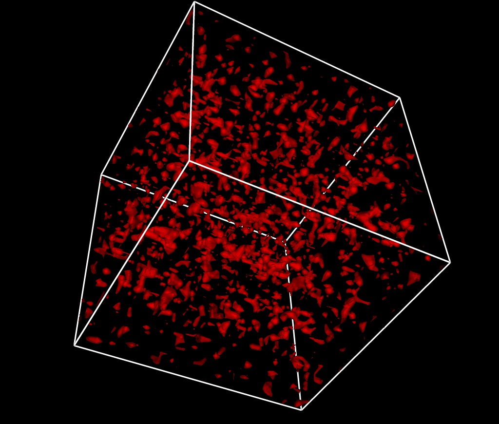
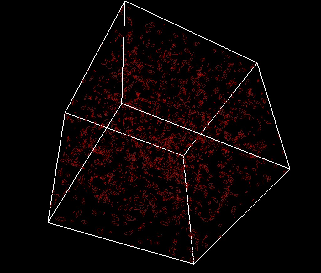
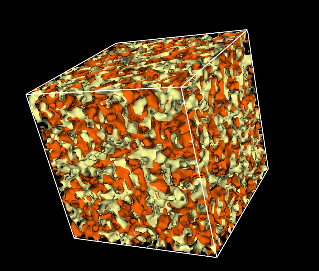
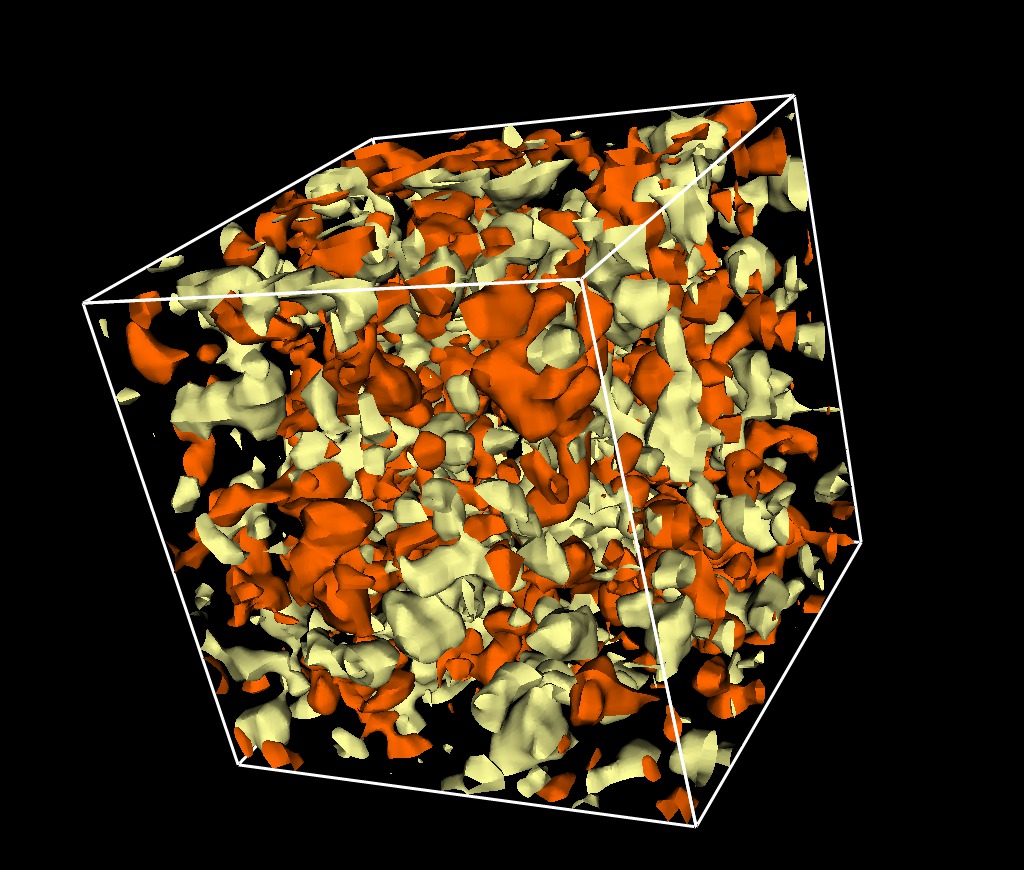
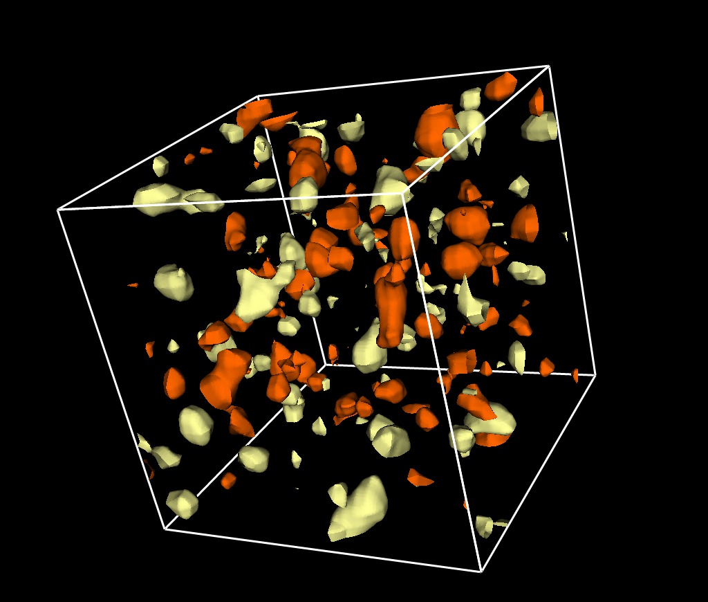
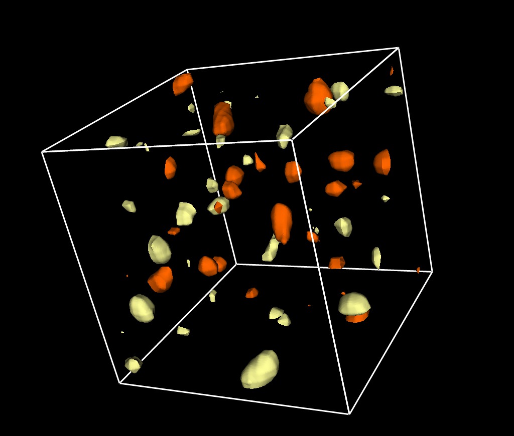
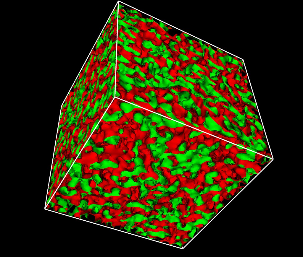
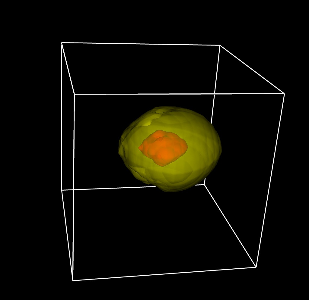
5.3 Topological charge density
Similarly to the average plaquette we can make images corresponding to the topological charge density.
To generate the topological change density we need to cool the gauge configurations (-cool) and then compute the topological charge (-topcharge_vtk):
The relavent code in “fermiqcd.cpp” is below:
topological_charge_vtk is defined in “fermiqcd_topological_charge.h”. The -1 arguments indicates we want to save all time slices. The actual code to compute the topological charge density is:
Here U.em is the eletro-magnetic field computed from U.
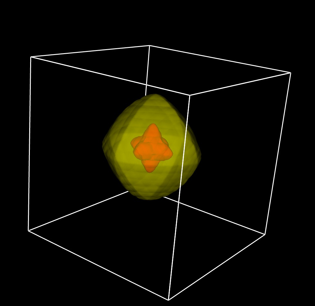
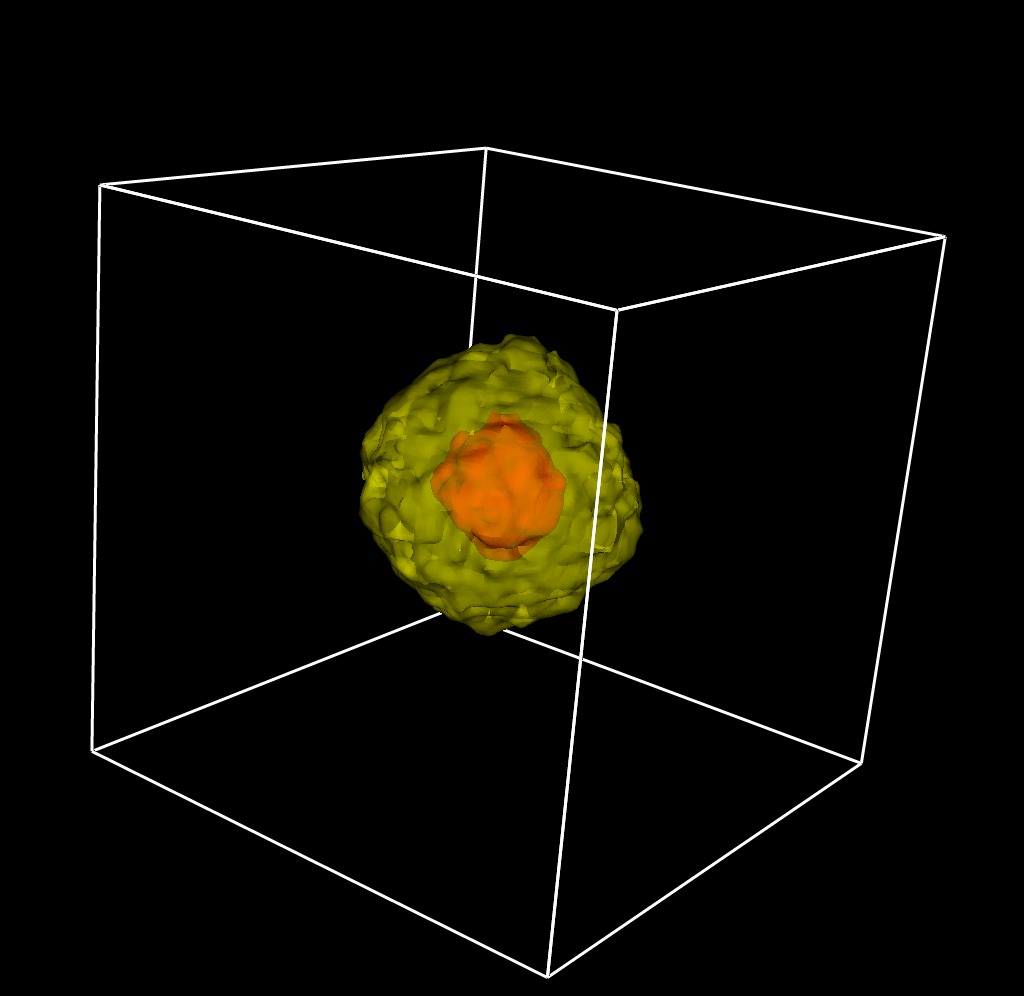
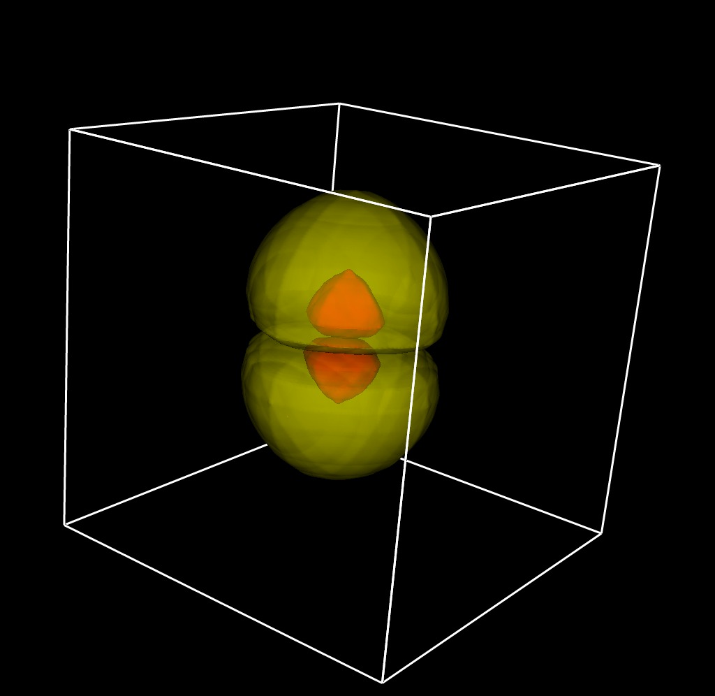
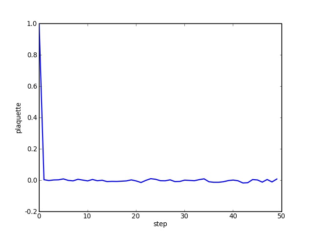
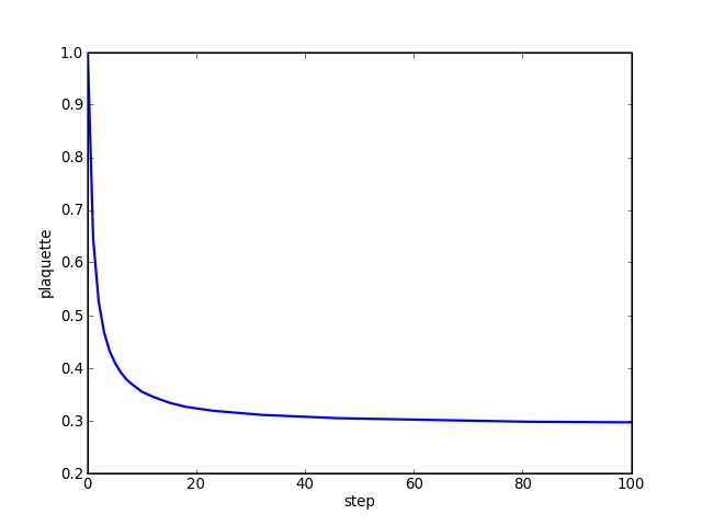
5.4 Cooling
Sometimes we may want to see the changes in the topological charge density as the configuration is cooled down. This requires computing the topological charge density at every cooling step. This can be done with the -cool_vtk option:
The -cool_vtk option creates VTK files ending in “cool00.vtk”, “cool01.vtk”,…, “cool49.vtk”. To make a smooth movie we do not break files into time-slices (no -s option) but instead we extract the same slice for every file (-r ’scalars_t0). Then we interpolate the frames (-i 9).
The above code generates JPEG images showing different stages of cooling of the data. You can see some of the images in fig. 6
 |
 |
 |
 |
The relevant code in “fermiqcd.cpp” is here:
The smearing algorithm is in the “topological_charge_vtk” file:
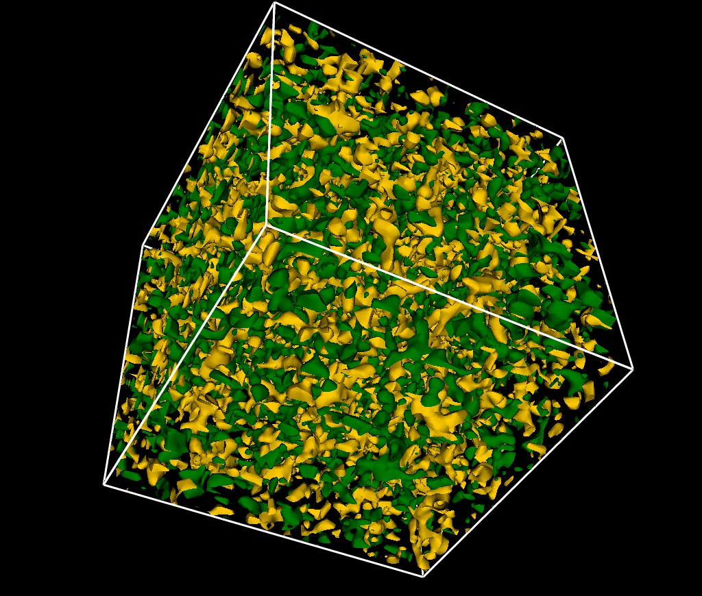
5.5 Polyakov lines
A Polyakov line is the trace of the product of the gauge links along the time direction, therefore it is a 3D complex field. Here we are interested in the real part only (the image part is qualitatively the same).
We can visualize Polyakov lines using the -polyakov_vtk option:
which we can convert to images with:
The output is show in fig. 7.
Here is the relevant code in “fermqcd.cpp”:
This code is a little different than the previous one. It creates a 3D lattice called space which is a time projection of the 4D space. While lives on the full lattice, leaves only on the 3D space. is a scalar field with two components (real and imaginary part of the Polyakov lines) which lives in 3D space.
5.6 Quark propagator
Given any gauge configuration we can visualize quark propagators in two ways. We can use the normal inverter and save the proprgator at the end of the inversion for each source/sink spin/color component:
(here using the bicgstab, the Stabilized Bi-Conjugate Gradient). Alternatively we can use a modified inverter which saves the components but also VTK visualization for the field components and the residue at each step of the inversion.
Fig. 8 shows different components of a quark propagator on a hot and a cold configuration.
 |
 |
 |
 |
 |
 |
From now on we assume the propagator has been computed and we reuse it.
5.7 Pion propagator
In a previous section, computed the zero momentum Fourier transform of the pion propagator. Now we want to visualize it for every point in space:
| (12) |
This can be done using the vtk=true attribute of the -pion option:
Notice the -quark...:load=true which reloads the previous propagator. We can now convert the pion VTK visualization into images using qcdutils_vis:
In this case the -i 9 option is used to interpolate between time-slices in case the images are to be assembled into a movie.
Examples of images are shown in fig.9
 |
 |
5.8 Meson propagators
A meson propagator is defined similarly to a pion propagator but it has a different gamma structure:
| (13) | |||||
| (14) |
We can visualized a Meson propagator using the following code:
and then process the VTK file as in the pion example. In this case indicates a verctor meson polarized along the axis.
5.9 Current insertions
We can also visualize the mass density and the charge density of a heavy-light meson by inserting an operator ( and respectively) in bewteen meson bra-kets.
| (15) | |||||
Here we measure the mass distribution for a static vector meson:
Using the same diagram we can compute the spatial distribution of by inserting the axial current () in between a static () and and a static ():
A sample image is shown in fig. 10.
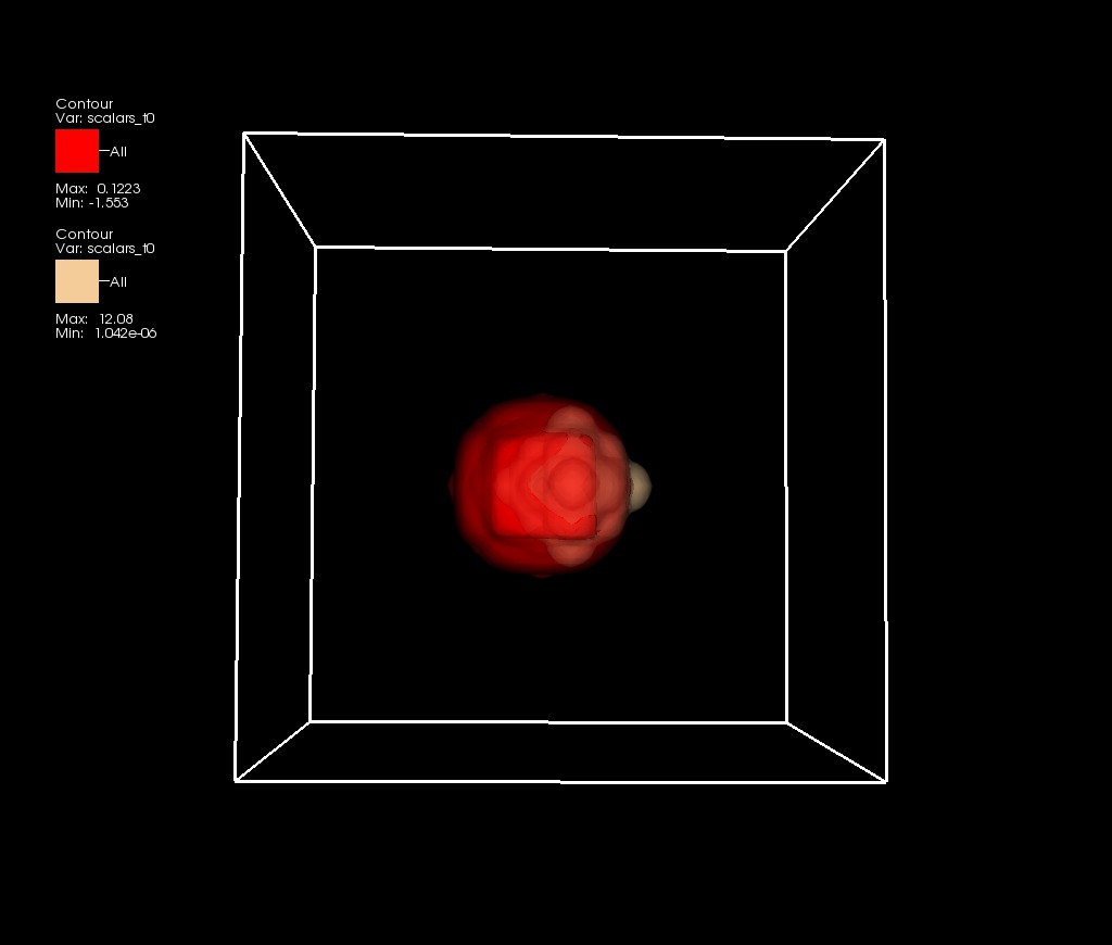
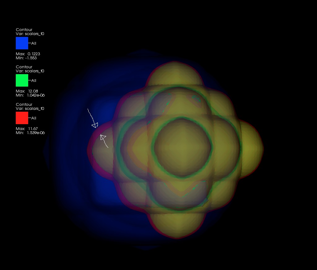
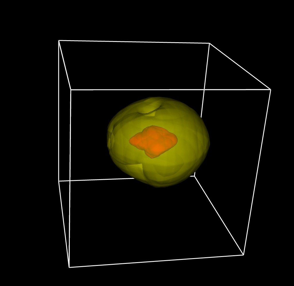
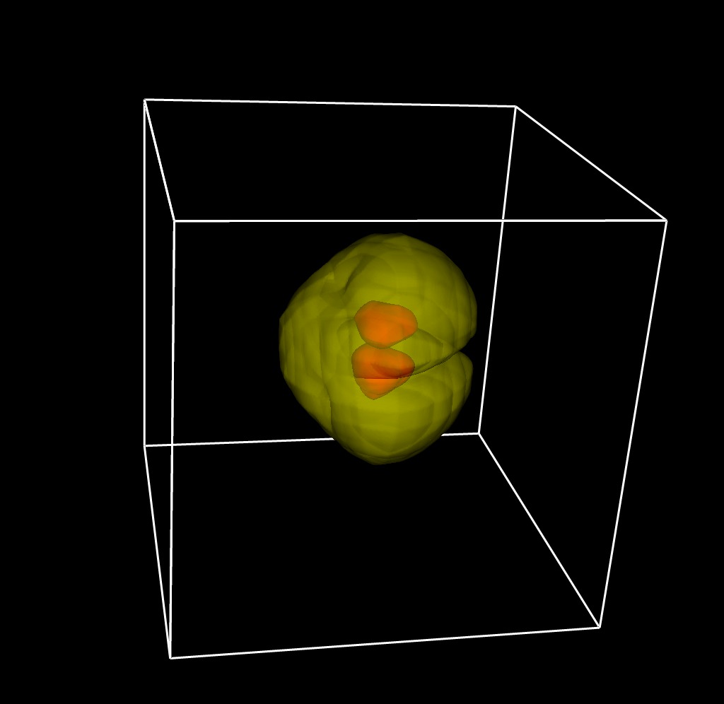
5.10 Localized instantons
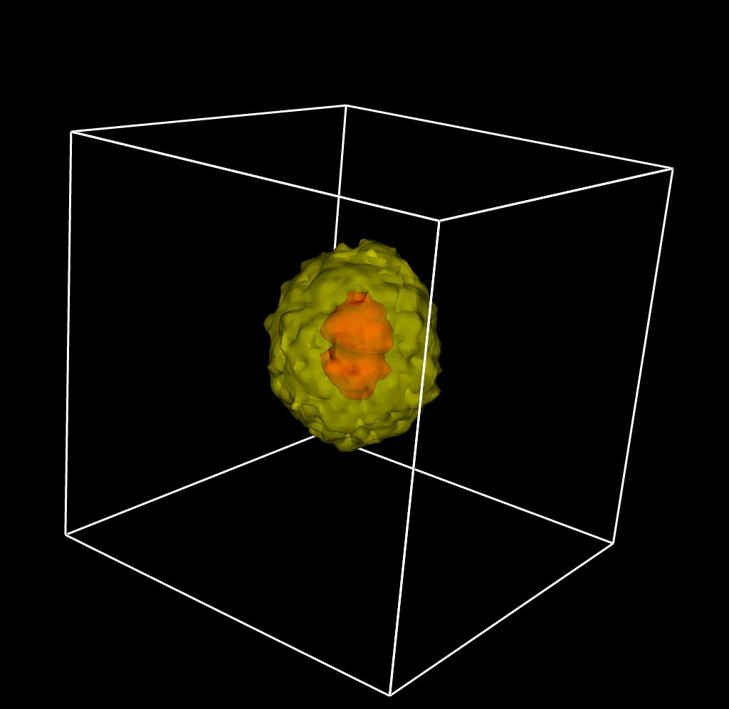
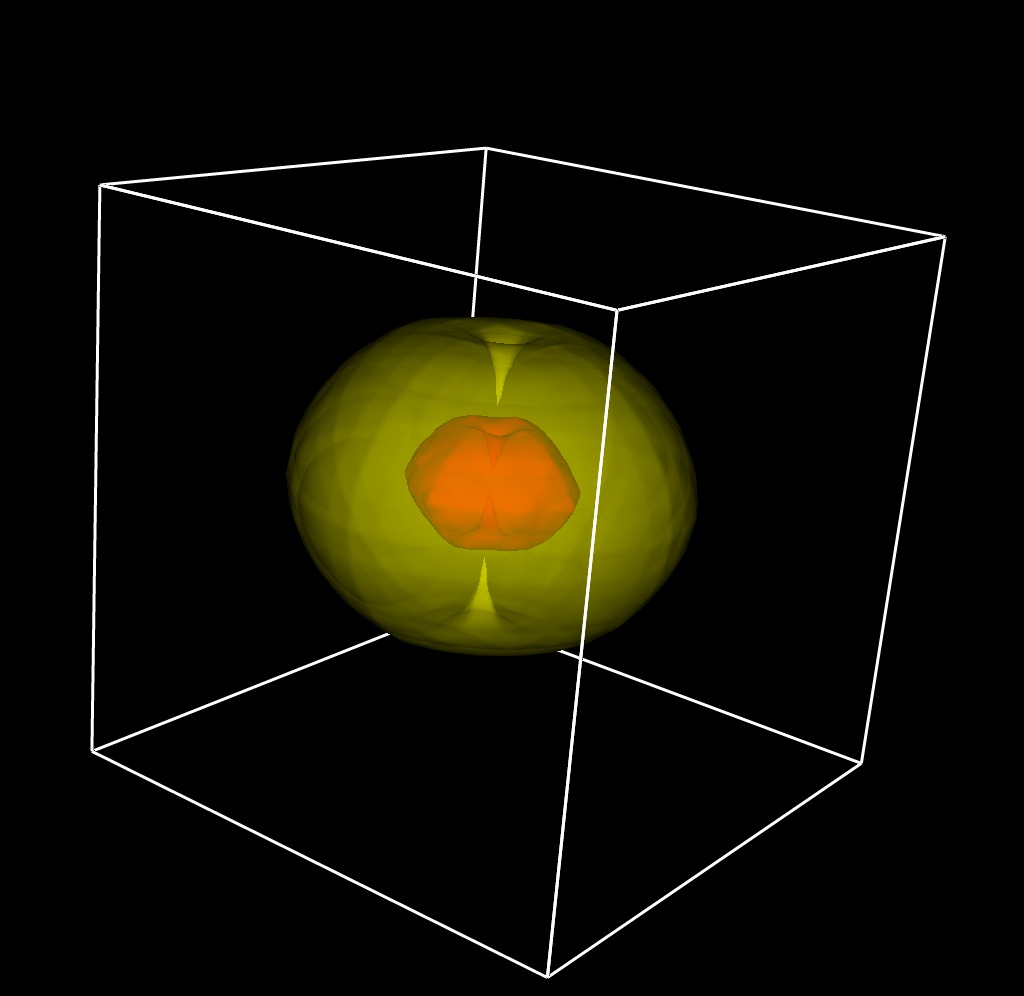
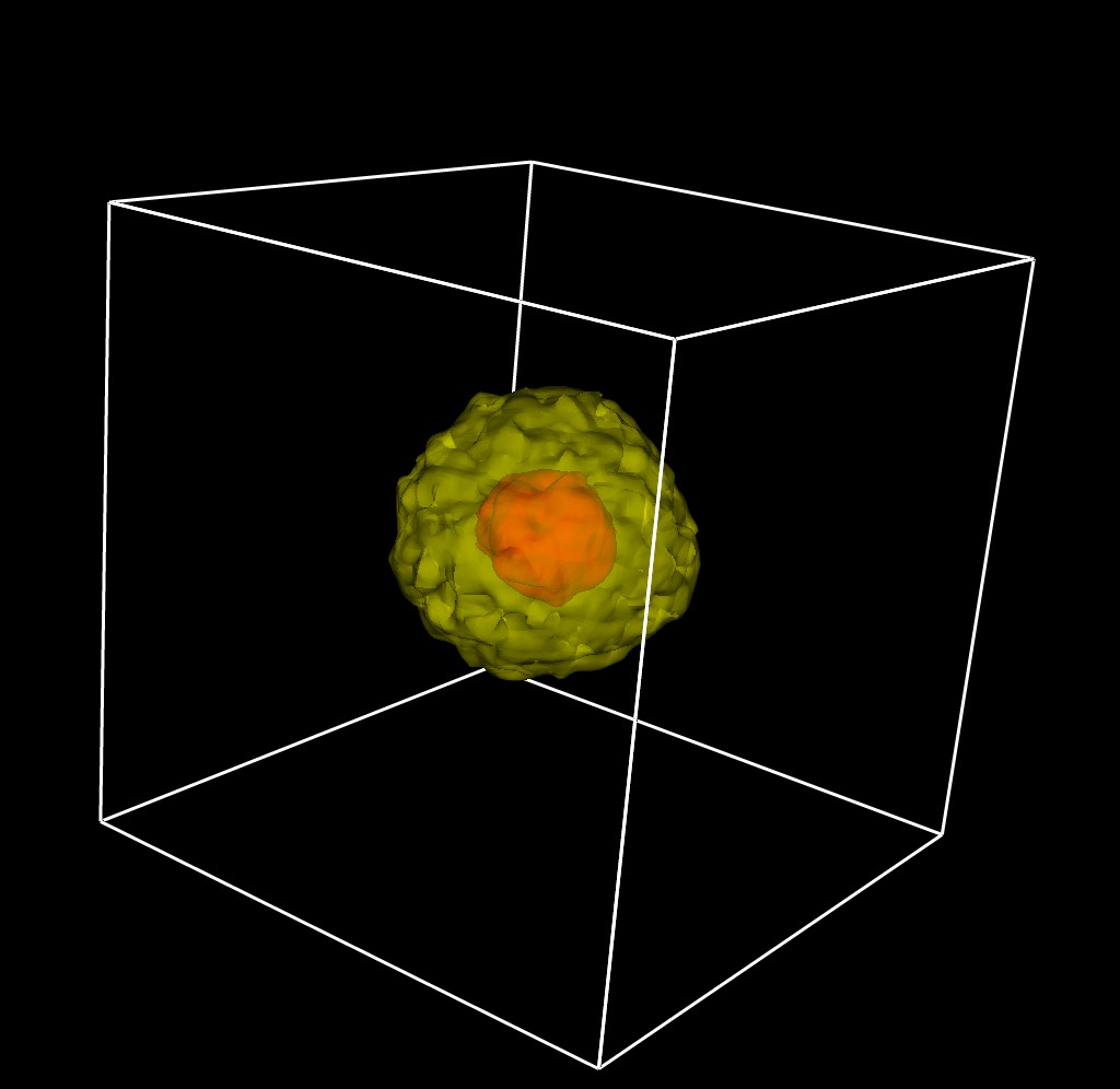
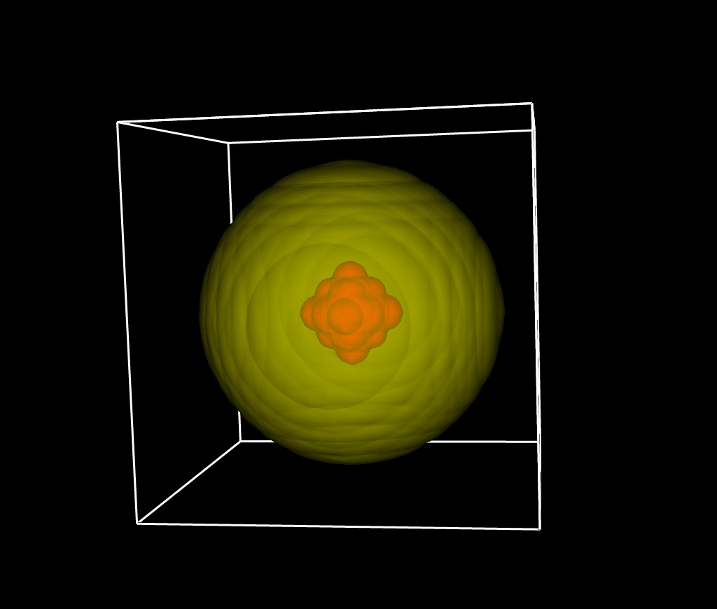
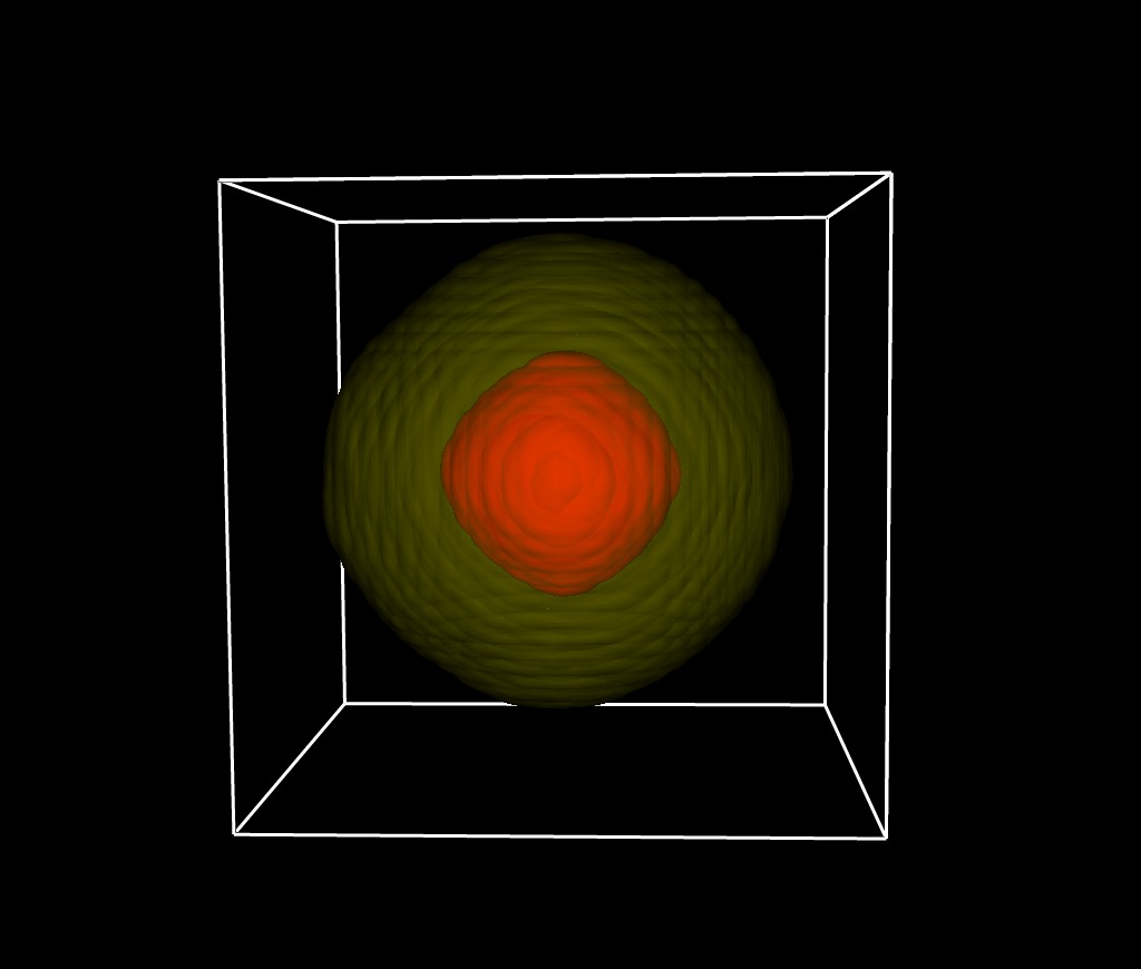
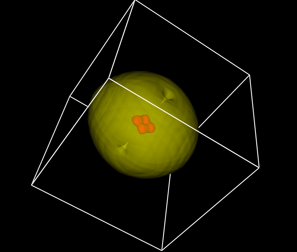
FermiQCD allows the creation of custom gauge configurations with localized topological charge. Here we consider the case of a pion propagator on a single gauge configuration in presence of one t’Hooft instanton (localized lump of topological charge). Here is the code:
This code places the center of the instanton at point and then computes a pion propagator with source on time slice 0 but spatial coordinates (center).
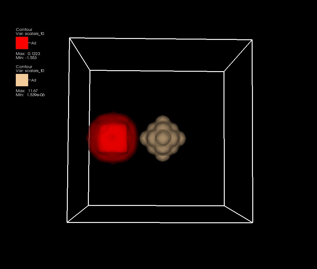
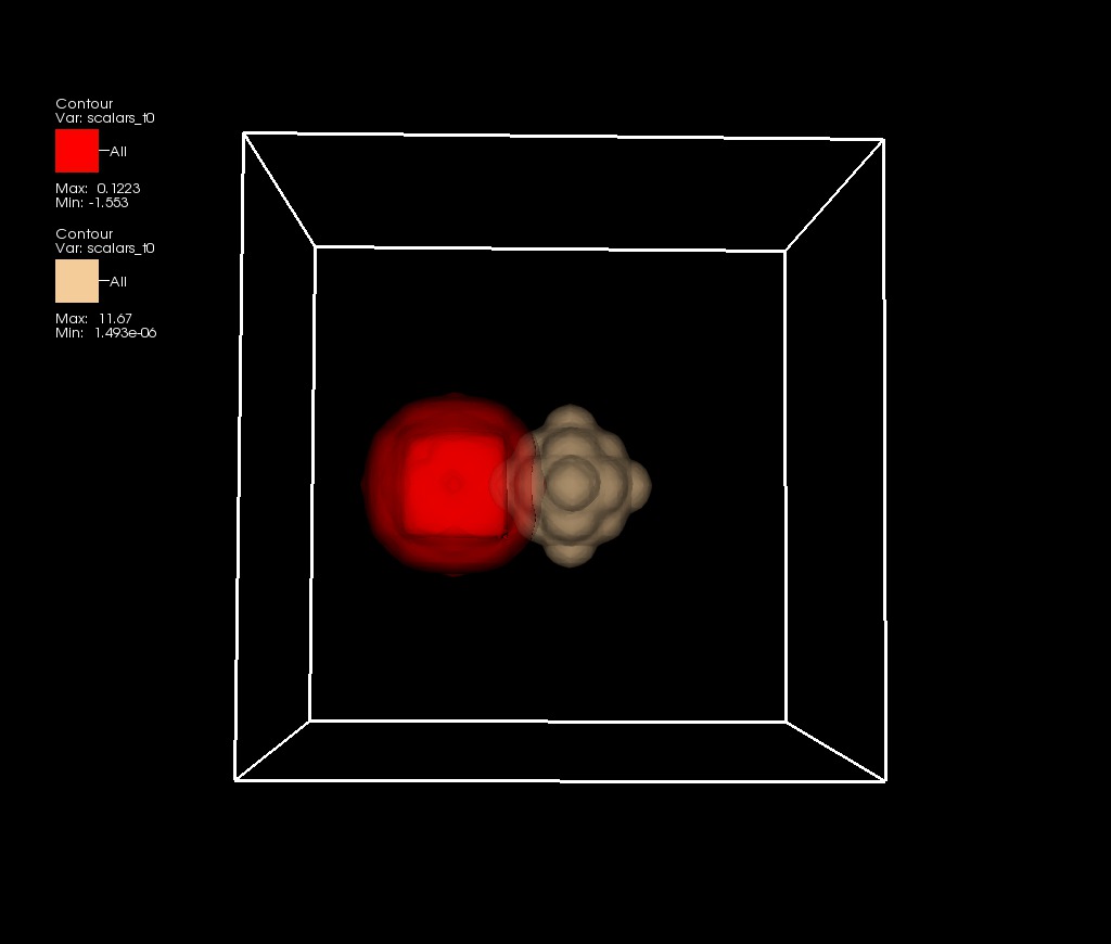
Fig. 11 show the pion propagator in presence of the instanton as the instanton nears the center of the propagator. Each image has been generated using the above command by placing the instanton at different locations. The last image shows a superposition of the pion propagator with and without the instanton in order to emphasize the difference. The difference is small but visible. The propagator retracts as the instanton nears. One may say that the quark interacts with the instanton and acquires mass thus making the propagator decrease faster when going through the instanton. Fig. 12 shows the effect of the instanton on individual components of the quark propagator.
 |
 |
 |
 |
|
 |
|
 |
|
 |
6 Analysis with qcdutils_boot.py, qcdutils_plot.py, qcdutils_fit.py
The console output of the qcdutils_run program consists of human readble text with comments and results of measurments performed on each gauge configuration. Here are some examples of measurements logged in the output:
qcdutils_boot.py is a tool that can extract the values for these measurements, aggregate them and analyze them in various ways. For example it computes the average and bootstrap errors [16] of any function of the measurements. qcdutils_plot.py is a tool to visualize the results of the analysis. It uses the Python matplotlib package, one of the most powerful and versatile plotting libraries available, although qcdutils_plot.py uses only a small subset of the available functionality.
Now, let us consider a typical Lattice QCD computation where one or more observables are measured on each Markov Chain Monte Carlo step (on each gauge configuration). We label the observables with (gauge configuration, 2-point correlation function for a given value of , etc.)
We also refer to each measurements with where labels the gauge configuration and labels the observable (same index as ). could be, for example, the plaquette on the th gauge configuration.
The expectation value of each one observable is computed by averaging its measurements over the MCMC steps:
| (16) |
Here is the number of the measurements. The statistical error on the average for this simple case can be estimated using the following formula:
| (17) |
Usually we are interested in the expectation value of non-trivial functions of the observables:
| (18) |
Often the are not normal distributed and may depend on each other therefore standard error analysis does not apply.
The proper technique for estimating the error on is the bootstrap algorithm. It consists of the following steps:
-
•
We build vectors of size N. The elements of these vectors are chosen at random, uniformly between .
-
•
For every we compute:
(19) -
•
Again for each we compute:
(20) -
•
We then sort the resulting values for .
-
•
We define the percent confidence interval as where and .
qcdutils_boot is a program that takes as input in the form of a mathematical expression where the are represented by their string pattern. It locates and extracts the corresponding values from the log files and stores them in a file called “qcdutils_raw.csv”. It computes the autocorrelation for each of the and stores them in “qcdutils_autocorrelation.csv”. It compute the moving averages for each of the and stores them in “qcdutils_trails.csv”. It generates the bootstrap samples and saves them in “qcdutils_samples.csv”. Finally it compute the mean and the 68% confidence level intervals and stores it “qcdutils_results.csv”.
Mind that these files are created in the current working directory and they are overwritten every time the qcdutils_boot is run. Move them somewhere else to preserve them.
Moreover, if the input expression for depends on wildcards, the program repeats the analysis for all matching expressions.
qcdutils_boot performs this analysis without need to write any code. It only needs the input in the syntax explained below and the list of log-files to analyze for data.
6.1 A simple example
Consider the output of one of the previous qcdutils_run:
In this case the observable is =“plaquette”. We can analyze it with
This produces the following output:
Notice that qcdutils_run takes three arguments:
-
•
A file name or file pattern (for example “run.log”)
-
•
An expression (for example “plaquette”).
-
•
A condition (optional)
Each of the argument must be enclosed in single quotes.
The represents and the are the names of observables in double quotes.
In ’"plaquette"’ the outer single quote delimits the expression and the term plaquette between double quotes, determines the string we want to parse from the in file.
qcdutils uses the observable name to find all the occurrences of
or
in the input files and maps them into where labels the occurrence. In this case we have a single observable (plaquette) so we use to label it.
The program opens the file or the files matching the file patterns and parses them for the values of the “plaquette” thus filling an internal table of s. It gives the output as the result:
Here “mean” is the mean of the expression “plaquette”. and are the 65% confidence intervals computed using the bootstrap.
Here is example of the content of the “qcdutils_results.csv” file for the average plaquette case:
In general it contains one row for each matching expression.
You can plot the content of the files generated by qcdutils_boot using qcdutils_plot:
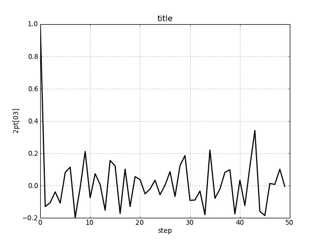
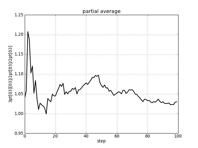
Here -r indicates that we want to plot the raw data, -a indicates we want a plot of autocorrelations, -t is for partial averages, and -b means we want a plot of bootstrap samples. qcdutils_plot loops over all the files reads the data in them and for each it makes one plot with raw data (), one with autocorrelations, one with partial averages. Then for each it makes one plot with the bootstrap samples, and one plot with the final results found in “qcdutils_results.csv”.
The plots are in PNG files which have a name prefix equal to the name of the data source file, followed by a serialization of the expression for or , depending on the case.
For example in the case of the plaquette, the autocorrelations and the partial averages are in the files:
and they are shown in fig. 13.
 |
 |
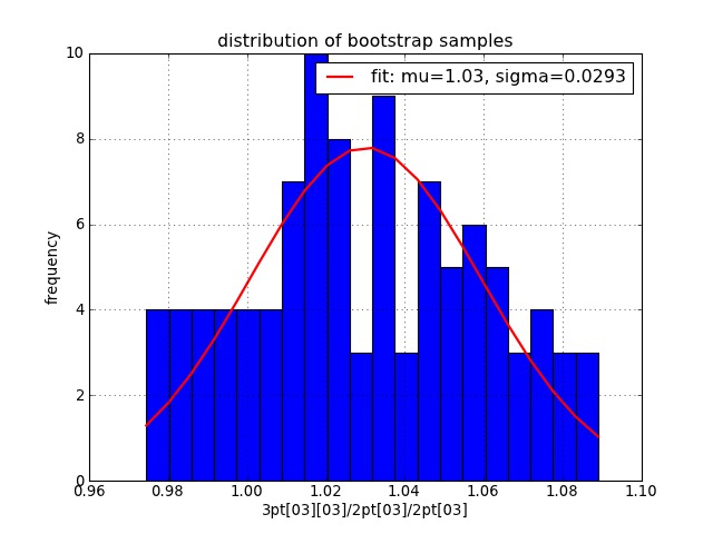
Similarly, if you want to bootstrap where is the plaquette you would run:
It produces output like this:
Notice that again the observable is identified for convenience by "plaquette". The double quotes are necessary to avoid naming conflicts between patterns and functions.
Also notice that running qcdutils_boot twice does not guarantee generating the same exact results twice. That is because the bootstrap samples are random.
6.2 2-point and 3-point correlation functions
In order to explain more complex cases we could generate 2- and 3- points correlation functions using something like:
For testing purposes can also run:
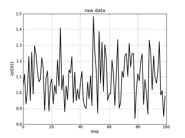
Where -t stands for test. This creates and analyzes a file called “test_samples.log” which contains random measurements for C2 and C3. Once this file is being created we can filter and study, for example, only the 2-point correlation function C2:
Notice that <t> means we wish to define a variable t to be used internally for the analysis and whose values are to be determined by pattern-matching the data. The t correspond to the of the previous abstract discussion. "C2[<t>]" matches C2[0] with , C2[1] matches with , etc.
The command above produces something like:
which we can plot as usual with
This produces about 60 plots. Some of them are shown in fig.14.
 |
 |
 |
We can as easily compute the log of C2 (for every t):
or the log of the ratio between C2 at two consecutive time-slices:
In this case we used two implicit variables t1 and t2 but we used the third argument of qcdutils_boot to set a condition to link the two. This produces the following output:
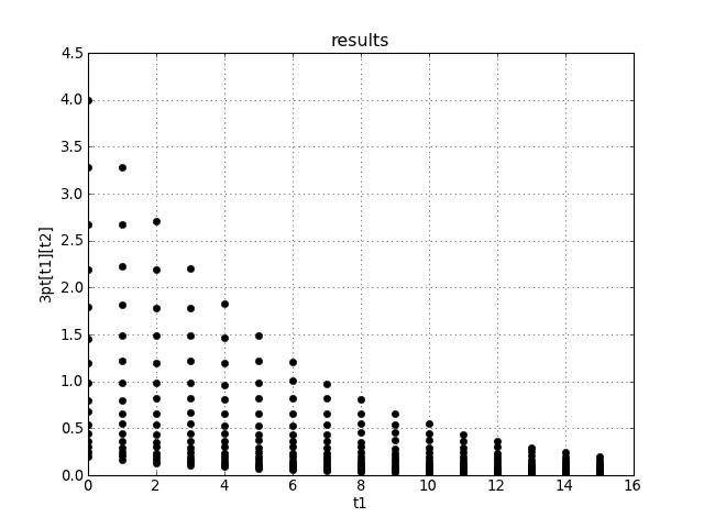
In the same fashion we can compute a matrix element as the ratio between a 3-point correlation function (C3) and a 2-point correlation function (C2):
 |
 |
6.3 Fitting data with qcdutils_fit.py
qcdutils_fit.py is a fitting and extrapolation utility. It can read and understand the output of qcdutils_boot.py. Internally it uses a “stabilized” multidimensional Newton method to minimize . It is stabilized by reverting to the steepest descent in case the Newton step fails to reduce the . The length of the steepest descent step is adjusted dynamically to guarantee that each step of the algorithm reduces the . The program accepts for input any function and any number of the parameters. It also accepts, optionally, Bayesian priors for those parameters and they can be used to further stabilize the fit [17]. A more sophisticated approach is described in ref. [18].
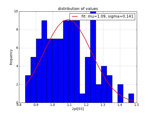
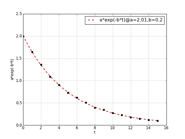
In Euclidean space C2 can be modeled by an exponential and is the mass of the lowest energy state which propagates between the source and the sink. Here is an example in which we fit C2 using a single exponential:
The input data is read from the output of qcdutils_boot. The expression in quotes is the fitting formula. You can name the fitting parameters as you wish (in this case a and b) but the other parameters (in this case t) must match the parameters defined in the argument of qcdutils_boot (<t>). The @ symbol separates the fitting function (left) from the initial estimates for the fitting parameters (on the right, separated by commas). Every parameter to be determined by the fit must have an initial value.
The output looks something like this:
qcdutils_fit.py also generates the plot of fig. 17 (left).
If C2 is a meson propagator, here represents the mass of the meson (of the lowest energy state with the same quantum numbers as the operator used to create the meson).
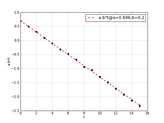
Similary we can analyze and fit the log of C2:
which produces something like:
and the plot of fig. 17 (right)
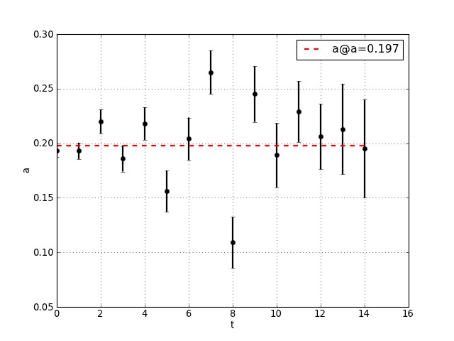
If our goal is obtaining we can also cancel the dependency in the analysis:
and obtain:
The generated plot is shown in fig. 18.
Notice that the variable names a and b are arbitrary and you can choose any name.
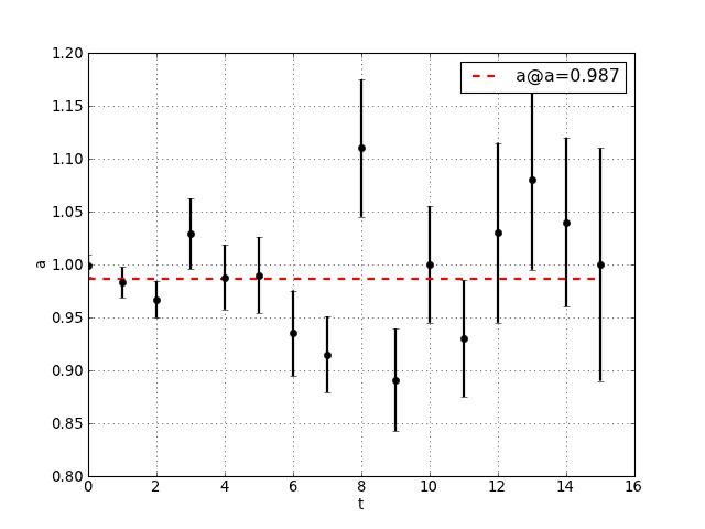
Similarly we can fit 3-point correlation functions:
In this case we have stabilized the plot with a Bayesian prior, indicated by _b. A variable starting with underscore indicates the uncertainty associated with our a priori knowledge about the corresponding variable without underscore. In other words b=0.3,_b=0.2 is equivalent to b=. The result of this fit yields something like:
A call to qcdutils_plot.py generates the plot of fig.19 (left)
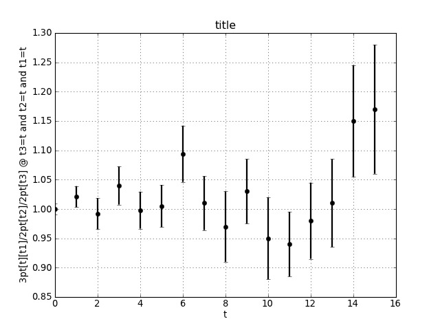
In order to extract a matrix element (for example a 4-quark operator) we fit the ratio between C3 and C2:
It produces output like:
It produces the plot in fig. 19 (right).
 |
 |
You can use qcdutils_fit.py to perform exatrapolations by using the -extrapolate command line option:
The extrapolated point will be added to the generated plot and represented by a square.
6.4 Dimensional analysis and error propagation
In this section we did not discuss error propagation but we have developed a utility called Buckingham which is avalable from:
http://code.google.com/p/buckingham/
It provides dimensional analysis, unit conversion, and aritmetic operation with error propgation. We plan to discuss it in a separate manual but we here provide one example of usage (from inside a Python shell):
(here pm stands for ) Buckingham supports 944 unit types (including eV) and their combinations.
Appendix A Filename conventions
Appendix B Help Pages
B.1 qcdutils_get.py
B.2 qcdutils_run.py
B.3 qcdutils_vis.py
B.4 qcdutils_vtk.py
B.5 qcdutils_boot.py
B.6 qcdutils_plot.py
B.7 qcdutils_fit.py
References
- [1] M. Di Pierro, J. Hetrick, S. Cholia, D. Skinner, PoS LAT2011, 2011
- [2] http://www.usqcd.org/ildg/
- [3] M. DiPierro, Comput.Phys.Commun. 141, 2001, (pp 98-148) [hep-lat/0004007]
- [4] M. Di Pierro, Nucl.Phys.Proc.Suppl.129:832-834, 2004 [http://fermiqcd.net]
- [5] http://www.vtk.org/
- [6] https://wci.llnl.gov/codes/visit/home.html
- [7] http://processingjs.org/
- [8] http://python.org
- [9] http://www.physics.utah.edu/~detar/milc
- [10] M. Creutz, Quarks, gluons and lattices, Cambridge University Press, 1985
- [11] I. Montvay and G. Münster, Quantum fields on a lattice Cambridge University Press, 1997
- [12] T. DeGrand and C. DeTar, Lattice Methods for Quantum Chromodynamics, World Scientific 2006
- [13] K. Wilson, K, Confinement of quark, Physical Review D 10 (8) 1974
- [14] C. Morningstar and M. Peardon, Phys.Rev.D56:4043-4061,1997
- [15] E. Eichten and B. Hill, Phys. Lett. B234 (1990) 51
- [16] B. Efron, The Annals of Statistics 7 (1), 1979
- [17] G. Lepage et al., Nucl.Phys.Proc.Suppl.106:12-20,2002 [arXiv:hep-lat/0110175v1]
- [18] M. Di Pierro, http://arxiv.org/abs/1202.0988v2