Scaling laws for the non-linear coupling constant of a Bose-Einstein condensate at the threshold of delocalization

Abstract

We explore the localization of a quasi-one-, quasi-two-, and three-dimensional ultra-cold gas by a finite-range defect along the corresponding ’free’-direction/s. The time-independent non-linear Schrödinger equation that describes a Bose-Einstein condensate was used to calculate the maximum non-linear coupling constant, $g_{max}$, and thus the maximum number of atoms, $N_{max}$, that the defect potential can localize. An analytical model, based on the Thomas-Fermi approximation, is introduced for the wavefunction. We show that $g_{max}$ becomes a function of $R_{0}\sqrt{V_{0}}$ for various one-, two-, and three-dimensional defect shapes with depths $V_{0}$ and characteristic lengths $R_{0}$. Our explicit calculations show surprising agreement with this crude model over a wide range of $V_{0}$ and $R_{0}$. A scaling rule is also found for the wavefunction for the ground state at the threshold at which the localized states approach delocalization. The implication is that two defects with the same product $R_{0}\sqrt{V_{0}}$ will thus be related to each other with the same $g_{max}$ and will have the same (reduced) density profile in the free-direction/s.

I Introduction

Since the experimental realization of Bose-Einstein condensates (BEC) in 1995 Anderson-MH95-269science198 ; Davis-KB95-75prl3969 , interest in the physics of ultracold atoms has grown and new areas of research have emerged. At the same time, it has renewed the interest in studying the collective dynamics of macroscopic ensembles of atoms occupying the same single-particle quantum state Griffin-A95-BEC ; Parkins-AS98-303pr1 ; Dalfovo-F99-71rmp463 . This, in turn, has created the need for new technology to study ultracold atoms. There are two technologies that motivate our present study; one is the atom chip, the second is sculptured optical field-based atom trapping. Both of which are capable of generating a myriad of trap geometries.

Our fundamental goal in this work is to determine the general scaling law that determines the maximum number of atoms that can be trapped by attractive defects described by 1-D, 2-D, and 3-D potentials when combined with confining harmonic atom traps. This corresponds to determining the limit at which the system transitions from a bound to a scattering state.

Our first motivation are the atom chips which play an important role in atomic physics, enabling the cooling and trapping of a BEC in a waveguide which is created by magnetic fields generated above patterned micro-wire circuits Fortagh-J07-79rmp235 . Atom chips have already enabled the study of matter-wave interference phenomena Cronin-AD09-81rmp1051 , and may improve other atomic measurement devices such as atomic clocks in the future. Ideally, the BEC is loaded/trapped in the transverse ground state, but is allowed free-space propagation along the third dimension. An ultra-cold wave-packet can then be transported through quasi-1-D waveguides due to the strong confinement in the two transverse dimensions Leanhardt-AE02-89prl040401 .

Our second motivation is the experimental realization of potential traps with different shapes that have been achieved using a rapidly moving laser beam that paints a time-averaged optical dipole potential. There, a BEC is created in arbitrary geometries Schnelle-SK08-16oe1405 ; Henderson-K09-11njp043030 . Effectively, the BEC confinement can be strong in one-dimension, reducing the BEC to be quasi-2-D in shape. The BEC can then be manipulated in these two-dimensions using a time-averaged potential. Both the atom chip and sculptured traps motivate us to explore a variety of shapes for a basic trap which includes a defect potential.

In the study of the structure of a gas of ultra-cold atoms, it is necessary to account for the interaction of the $N$ atoms. That is, each atom moves in an average field due to the other $N-1$ atoms that surrounds it. The properties of a BEC at $T=0$ is well-described by a mean-field approximation which results in a non-linear Schrödinger equation (NLSE) for the single-particle orbitals Esry-BD97-55pra1147

$$i\frac{\partial\>}{\partial t}\Psi(\mathbf{r},t)=\left[-\frac{1}{2}\nabla^{2}+V(\mathbf{r})+g_{3}\lvert\Psi(\mathbf{r},t)\rvert^{2}\right]\Psi(\mathbf{r},t).$$ (1)

The nonlinear coupling constant characterizes the short-range pairwise interactions, and is given for $N$ bosons by $g_{3}=4\pi{a_{s}}(N-1)/a_{\perp}$ according to (number conserving) Hartree-Fock theory Esry-BD97-55pra1147 . This constant depends on the s-wave atom-atom scattering length, $a_{s}$, of two interacting bosons. Note that alternative treatments give $g_{3}\propto N$, and then the above NLSE is known as the Gross-Pitaevskii equation (GPE) Dalfovo-F99-71rmp463 . Eq. (1) has been written in oscillator units (o.u.), with lengths $a_{\perp}=\sqrt{\hbar/m\omega_{\perp}}$ for a chosen frequency $\omega_{\perp}$ and $m$ being the mass of the individual atoms that compose the BEC. The energy is thus given in units of the oscillator energy $\hbar\omega_{\perp}$, and time in units of $1/\omega_{\perp}$. Back in S.I. units, $g_{3}^{SI}=4\pi\hbar^{2}a_{s}(N-1)/m=\hbar^{2}g_{3}/(a_{\perp}m)$.

For the present study, we chose time-independent potentials for $V(\mathbf{r})$ with one of three structures:

$$V_{1}(x,y,z) = \frac{1}{2}m\omega_{\perp}(y^{2}+z^{2})+V^{\prime}_{1}(x)\>,$$ (2)

$$V_{2}(x,y,z) = \frac{1}{2}m\omega_{\perp}(z^{2})+V^{\prime}_{2}(x,y)\>,$$ (3)

$$V_{3}(x,y,z) = V^{\prime}_{3}(x,y,z)\>.$$ (4)

That is, we partition the defect potential $V^{\prime}$, which is of interest here, from the transverse harmonic trap potential applied at a frequency $\omega_{\perp}$.

The $V^{\prime}_{1}$ defect potentials, for example, can be generated by a local modification of the transverse waveguide confinement, such as a constriction Jaaskelainen-M02-66pra023608 ; Lahaye-T03-8cnsns315 ; Leboeuf-P03-68pra063608 ; Koehler-M05-72pra023603 or a local curvature Leboeuf-P01-64pra033602 ; Bromley-MWJ03-68pra043609 ; Bromley-MWJ04-69pra053620 . Whether a defect potential acts as an obstacle or a sink, a wave-packet will interfere with, and possibly lose atoms as it goes through the defect due to the non-linearity Ernst-T10-81pra033614 ; Gattobigio-GL10-12njp085013 , changing the interaction for any subsequent atom. In general, propagation through a perturbation in a 1-D waveguide results in unwanted transverse excitations of the BEC Leanhardt-AE02-89prl040401 ; Bromley-MWJ04-70pra013605 .

The presence of a transverse-$\omega_{\perp}$ potential allows for the reduction of the NLSE from 3-D to either a 2-D or 1-D form. In the 1-D, or $V_{1}$, case we assume that the tight-waveguide limit applies where the longitudinal-($x$) size of the BEC is larger than its transverse-($y,z$) cross section. This allows for us to integrate out the transverse dimensions which are energetically frozen in the harmonic ground state. This results in a 1-D NLSE,

$$i\frac{\partial\>}{\partial t}\Psi(x,t)=\left[-\frac{1}{2}\frac{\partial^{2}\>}{\partial x^{2}}+V^{\prime}_{1}(x)+g_{1}|\Psi|^{2}\right]\Psi(x,t)$$ (5)

with an effective 1-D coupling constant, $g_{1}=g_{3}/(2\pi)=2{a_{s}}(N-1)/a_{\perp}$. Back in S.I. units $g_{1}^{SI}=g_{3}^{SI}/(2\pi a_{\perp}^{2})$, and note that the intermediate reduction from 3-D to 2-D gives a similar NLSE with constant $g_{2}=g_{3}/\sqrt{2\pi}$.

By systematically adding more and more atoms with $a_{s}>0$ into the potential, at some $g_{3,max}$ the total 3-D eigenenergy, $\varepsilon_{3}$, of the system becomes null with respect to the transverse trap energy Leboeuf-P01-64pra033602 . For the three geometries in Eq. (2), this corresponds to $\varepsilon_{3}=\hbar\omega_{\perp}$, $\varepsilon_{3}=\frac{1}{2}\hbar\omega_{\perp}$ or $\varepsilon_{3}=0$. Determining the $g_{3,max}$ is non-trivial since at this point the system is no longer bound, the delocalized atoms can reach $|\mathbf{r}|=\infty$, and thus cannot be represented by a square-integrable wavefunction, and needs to be considered as the limit $\varepsilon_{3}\to 0$ from below.

The first analytical approximations for $g_{1,max}$ were simultaneously derived by Carr et al. Carr-LD01-64pra033603 and Leboeuf and Pavloff Leboeuf-P01-64pra033602 . Carr et al. Carr-LD01-64pra033603 solved the 1-D NLSE for a finite square-well finding localized solutions when the 1-D eigenenergy, $\varepsilon_{1}<0$. The transition at $\varepsilon_{1}=0$ was found in terms of an approximate expression for $g_{1,max}$ containing $R_{0}\sqrt{V_{0}}$ terms where the potential well has depth, $V_{0}$, and width, $2R_{0}$. (see Eq. (21) of Ref. Carr-LD01-64pra033603 ) which our results will show agreement with.

Leboeuf and Pavloff Leboeuf-P01-64pra033602 derived approximate expressions in terms of the maximum number of atoms that a 1-D potential could support based on the area enclosed by the potential, $\lambda=|\int_{-\infty}^{\infty}V^{\prime}_{1}(x)dx|$. In the low-density BEC limit, this translates from their $\hbar=m=1$ units to $g_{1,max}=2\lambda$ when in o.u.. They argued that, in general, this was expected ’to be very accurate’ despite using a $V^{\prime}_{1}(x)\to-\lambda\delta(x)$ approximate mapping. They did not explicitly validate their formula against explicit calculations. More recent analytical work by Seaman et al. Seaman-BT05-71pra033609 showed that, for a potential $V^{\prime}_{1}(x)=-\beta\delta(x)$, the $g_{1,max}=4\beta$ exactly. Our results agree with Seaman et al., in that, there is a factor of 2 underestimate in the treatment of Leboeuf and Pavloff in the limit of weak potentials. Our results also agree with Carr et al. Carr-LD01-64pra033603 which show that the Leboeuf and Pavloff expression has a factor of 2 overestimate in the limit of strong potentials.

The final paper of direct relevance to the present study is that of Adhikari Adhikari-SK07-42ejpd279 who solved the 3-D NLSE with a finite spherical-well potential, and computed the maximum nonlinear coupling constant, $g_{3,max}$. There, a 3-D variational ansatz was applied and an almost linear relation was plotted (see their Fig. (3)) in which $g_{3,max}\propto V_{0}$, the depth of the well. Adhikari noted that the variational ansatz underestimates the magnitude of $g_{3,max}$, but gave no calculations to quantify this.

Furthermore, of particular interest is that Adhikari Adhikari-SK07-42ejpd279 also applied a Thomas-Fermi approximation (TFA) to compute, in our notation, $g_{3,max}=4\pi R_{0}^{3}V_{0}/3$. In their paper it is noted the TFA “is inadequate for calculating” $g_{3,max}$, leading to a “much smaller” value than the variational ansatz. It was thus surprising to us when we applied the same TFA in preliminary 1-D calculations LopezMiranda-JA09-XXIXicpigPA1.3 , and found excellent agreement with explicit calculations of $g_{1,max}$. In the present paper we find that the TFA gives $g_{2,max}$ and $g_{3,max}$’s accurately for all of the potential defects that we consider. Our 3-D results show that both the $g_{3,max}$ results and conclusions of Adhikari’s variational ansatz Adhikari-SK07-42ejpd279 are not accurate.

In this work, we present some analytical results in Sec. II using the TFA for $i=$ 1-, 2-, and 3-D defect potentials and deduce universal scaling rule properties for $g_{i,max}$ and the wavefunction (density profiles). The $g_{i,max}$ is seen to follow a scaling law that depends on $R_{0}\sqrt{V_{0}}$, across a wide range of width parameters and potential shapes. In the 1-D case, we present results for a square-well, triangle, truncated harmonic, truncated double harmonic, and truncated half circle defect. We have previously published results of four of these trap shapes solely in 1-D for $g_{1,max}$ LopezMiranda-JA09-XXIXicpigPA1.3 . Here, we expand and extend that work into 2-D and then 3-D for a wider range of potential defects. For the 2-D traps case, we study a rectangle well, truncated harmonic and pyramid defect. For a 3-D trap we use a spherical, rectangular cuboid and a truncated harmonic well defect. Furthermore, we report a scaling rule for the wavefunction in terms of the range of the potential. In Sec. III, we present our numerical approach to solve the NLSE based on a finite-difference method on a numerical lattice and a Gauss-Seidel procedure to obtain the numerical ground state on the lattice for the 1-, 2-, and 3-D NLSE. In Sec. IV, we present and discuss our results. Finally, in Sec. V we present our conclusions.

II Analytic results using the Thomas-Fermi approximation

The TFA considers the limit of strong interactions between atoms that form an ultra-cold BEC and allows for some useful expressions for the single-particle wavefunction to be obtained Edwards-M95-51pra1382 ; Baym-G96-76prl6 . A BEC is said to be in the Thomas-Fermi (TF) regime when the interaction energy dominates over the zero-point energy Edwards-M95-51pra1382 ; Baym-G96-76prl6 . The TF states are strictly localized by a potential, and thus their behavior was not initially expected to be able to mimic the NLSE localized states as they approach delocalization as was previously noted by Adhikari Adhikari-SK07-42ejpd279 . Instead, we will show that this approximation gives us a general ($R_{0}\sqrt{V_{0}}$)-based scaling law that agrees with the numerical NLSE solutions.

The TFA neglects the kinetic energy in the NLSE, and therefore the time-independent NLSE in either $i\in 1,2,3$ dimensions becomes

$$\left[V^{\prime}_{i}(\mathbf{r})+g_{i}^{TF}|\Psi_{TF}(\mathbf{r})|^{2}\right]\Psi_{TF}(\mathbf{r})=\varepsilon_{i}\Psi_{TF}(\mathbf{r}),$$ (6)

where $\varepsilon_{i}$ is the $i$-D single-particle orbital energy. The maximum nonlinear coupling constant due to the defect potential occurs when $\varepsilon_{i}\to 0$, so Eq. (6) reduces to

$$\Psi_{TF}(\mathbf{r})=\lim_{\varepsilon_{i}\to 0}\sqrt{\frac{\varepsilon-V^{\prime}_{i}(\mathbf{r})}{g_{i}^{TF}}}=\sqrt{\frac{-V^{\prime}_{i}(\mathbf{r})}{g^{TF}_{i,max}}}.$$ (7)

Through normalization, $\int_{\Omega}|\Psi(\mathbf{r})|^{2}dr^{i}=1$, one obtains that $g^{TF}_{i,max}$ satisfies the relation

$$g^{TF}_{i,max}=-\int_{\Omega}V^{\prime}_{i}(\mathbf{r})dr^{i}\,,$$ (8)

where $\Omega$ is the contour around the defect where $V^{\prime}_{i}(\mathbf{r})=0$. Thus, the non-linear coupling parameter $g^{TF}_{i,max}$ just depends on the extension $\Omega$ (area or volume for the 2- or 3-D case) of the defect potential in the TFA. Hence, for a given scattering length $a_{s}$, atom mass $m$ and transverse frequency $\omega_{\perp}$, the corresponding maximum number of atoms trapped by a defect, $N_{max}$, can be determined.

II.1 One-dimensional case

We consider here the following five 1-D defect potential shapes. In all of these cases, $V_{0}>0$ is the strength of the potential and $2R_{0}$ is the width of the potential region. A square potential

$$V_{1,s}^{\prime}(x)=\left\{\begin{array}[]{cl}-V_{0}&,|x|<R_{0},\\ 0&,|x|>R_{0},\\ \end{array}\right.$$ (11)

a half circle potential trap

$$V_{1,c}^{\prime}(x)=\left\{\begin{array}[]{cc}-V_{0}\sqrt{1-\left(\frac{x}{R_{0}}\right)^{2}}&,|x|<R_{0},\\ 0&,|x|>R_{0}.\\ \end{array}\right.$$ (14)

a (truncated) harmonic potential trap

$$V_{1,h}^{\prime}(x)=\left\{\begin{array}[]{cc}-V_{0}\left[\left(\frac{x}{R_{0}}\right)^{2}-1\right]&,|x|<R_{0},\\ 0&,|x|>R_{0},\\ \end{array}\right.$$ (17)

a symmetric double harmonic potential trap

$$V_{1,2h}^{\prime}(x)=\left\{\begin{array}[]{cc}4V_{0}\left(\left(\frac{x}{R_{0}}\right)^{2}+\frac{x}{R_{0}}\right)&,-R_{0}<x<0,\\ 4V_{0}\left(\left(\frac{x}{R_{0}}\right)^{2}-\frac{x}{R_{0}}\right)&,0<x<R_{0},\\ 0&,|x|>R_{0},\\ \end{array}\right.$$ (21)

and a triangle potential

$$V_{1,t}^{\prime}(x)=\left\{\begin{array}[]{cc}-V_{0}\left(1+\frac{x}{R_{0}}\right)&,-R_{0}<x<0,\\ -V_{0}\left(1-\frac{x}{R_{0}}\right)&,0<x<R_{0},\\ 0&,|x|>R_{0},\\ \end{array}\right.$$ (25)

From Eq. (8), each potential gives, respectively, a non-linear coupling constant given by

$$g^{TF}_{1,max}=\left\{\begin{array}[]{cl}2(R_{0}\sqrt{V_{0}})^{2}/R_{0},&\mathrm{square-well}\\ \pi(R_{0}\sqrt{V_{0}})^{2}/(2R_{0}),&\mathrm{circle}\\ 4(R_{0}\sqrt{V_{0}})^{2}/(3R_{0}),&\mathrm{harmonic}\\ 4(R_{0}\sqrt{V_{0}})^{2}/(3R_{0}),&\mathrm{double}\\ (R_{0}\sqrt{V_{0}})^{2}/R_{0},&\mathrm{triangle}\,.\end{array}\right.$$ (31)

Thus, it seems that $g_{1,max}^{TF}$ has a universal dependence on $R_{0}\sqrt{V_{0}}$ in the 1-D case, independent of the shape of the defect potential, i.e $g_{i}=f(R_{0}\sqrt{V_{0}})$.

A more general, but still approximate, expression for the nonlinear coupling constant that includes the kinetic energy term in the NLSE has been found by Carr et al. for the one-dimensional square-well, (see Eq. (21) in Ref. Carr-LD01-64pra033603 ), and is given by

$$g_{1,max}(\gamma)\!\approx\!\frac{\gamma}{R_{0}}\!\left[\sqrt{2}\left(\frac{e^{-\sqrt{2}\gamma}}{1+2e^{-\sqrt{2}\gamma}-e^{-2\sqrt{2}\gamma}}\right)\!+\!2\gamma\right],$$ (32)

where $\gamma=R_{0}\sqrt{V_{0}}$. In the limit when $\gamma\gg 1$, the exponentials can be neglected and Eq. (32) reduces to $g_{1,max}(\gamma)=2(R_{0}\sqrt{V_{0}})^{2}/R_{0}$. This agrees with the TFA found for the case of the square-well (first line in Eq. (31)). The other defect potentials considered here appear to have no equivalent analytical expression in the literature.

II.2 Scaling of the 1-D NLSE

Due to the chosen geometries of the defects, one can make an additional change of variables to $\bar{x}=x/R_{0}$ and $\bar{\varepsilon}_{1}=\varepsilon_{1}/V_{0}$ obtaining the following reduced 1-D NLSE,

$$\left[-\frac{1}{2V_{0}R_{0}^{2}}\frac{\partial^{2}\>}{\partial\bar{x}^{2}}+\bar{V}(\bar{x})+\frac{g_{1}R_{0}}{V_{0}R_{0}^{2}}|\Phi|^{2}\right]\Phi(\bar{x})=\bar{\varepsilon}_{1}\Phi(\bar{x}),$$ (33)

where $\Phi(\bar{x})=\sqrt{R_{0}}\Psi(\bar{x})$ such that $\Phi(\bar{x})$ remains normalized in the $\bar{x}$ range. Here, $\bar{V}(\bar{x})=V^{\prime}_{1}(\bar{x})/V_{0}$ is the reduced defect potential with a maximum strength of $-1$ and defined only in the range $|\bar{x}|<1$.

For large values of $(R_{0}\sqrt{V_{0}})^{2}$, one notices that the kinetic energy term in Eq. (33) can be neglected, justifying the TFA when $R_{0}$ and/or $V_{0}$ are large. The non-linear term can not be neglected since $g_{1}=f(R_{0}\sqrt{V_{0}})$, as previously mentioned. The equivalent of Eq. (8) in these reduced units can be thought of as a shape factor, $\alpha$, given by the area under the reduced potential:

$$\alpha_{1D}\equiv\frac{g_{1,max}^{TF}R_{0}}{(R_{0}\sqrt{V_{0}})^{2}}=-\int_{|\bar{x}|<1}\bar{V}(\bar{x})d\bar{x}$$ (34)

This shape factor takes the values of $2,\,\pi/2,\,4/3,\,4/3$, and $1$ for each 1-D potential, respectively.

On the other hand, from Eq. (33), we now note that defects of the same type with the same $R_{0}\sqrt{V_{0}}$ have the same $g_{1,max}$ and the same reduced wavefunction, therefore, there is a fundamental relation between the density profile for different parameters. We will discuss below some further examples where this scaling law holds.

II.3 Two-dimensional case

For the case of a two-dimensional traps, the time-independent NLSE is given by

$$\Big{\{}-\frac{1}{2}\left[\frac{\partial^{2}}{\partial x^{2}}+\frac{\partial^{2}}{\partial y^{2}}\right]+V^{\prime}_{2}(x,y) +$$ (35)

$$g_{2}|\Psi|^{2}\Big{\}}\Psi(x,y) = \varepsilon_{2}\Psi(x,y)\,.$$

Thus, the application of the TFA again gives the following expression for the 2-D coupling constant at delocalization

$$g_{2,max}^{TF}=-\int_{\Omega}V^{\prime}_{2}(x,y)\,dxdy\,.$$ (36)

In this case we have considered the following three 2-D defect potentials: a rectangular well

$$V^{\prime}_{2}(x,y)=\left\{\begin{array}[]{cc}-V_{0}&,\mathrm{if}\;|x|<R_{x}\;\mathrm{and}\;|y|<R_{y}\\ 0&,\mathrm{if}\;|x|>R_{x}\;\mathrm{and}\;|y|>R_{y}\,,\\ \end{array}\right.$$ (37)

a truncated harmonic (parabolic) well with circular base

$$V^{\prime}_{2}(x,y)=\left\{\begin{array}[]{cc}-V_{0}(R_{0}^{2}-x^{2}-y^{2})/R_{0}^{2}&,\mathrm{if}\;\sqrt{x^{2}+y^{2}}<R_{0}\\ 0&,\mathrm{otherwise}\,,\\ \end{array}\right.$$ (38)

thirdly, a pyramid (triangle) potential

$$V^{\prime}_{2}(x,y)=\left\{\begin{array}[]{rr}-V_{0}\frac{(y+R_{y})}{R_{0}}&,y<|x|\,,\,-R_{y}<y<0\\ V_{0}\frac{(y-R_{y})}{R_{0}}&,y>|x|\,,\,R_{y}>y>0\\ -V_{0}\frac{(x+R_{x})}{R_{0}}&,|y|<x\,,\,-R_{x}<x<0\\ V_{0}\frac{(x-R_{x})}{R_{0}}&,|y|>x\,,\,R_{x}>x>0\\ 0&,\mathrm{otherwise}\\ \end{array}\right.$$ (39)

where each line represents the equation on each pyramid wall.

II.4 Scaling of the 2-D NLSE

Following a procedure similar to the 1-D case, the 2-D NLSE can be further rewritten in terms of the reduced variables. Making the change of variables: $\bar{x}=x/\sqrt{R_{x}R_{y}}$, $\bar{y}=y/\sqrt{R_{x}R_{y}}$, $\Phi=\sqrt{R_{x}R_{y}}\Psi$, and $\bar{\varepsilon}_{2}=\varepsilon_{2}/V_{0}$, one obtains

$$\Big{\{}-\frac{1}{2V_{0}R_{x}R_{y}}\left[\frac{\partial^{2}}{\partial\bar{x}^{2}}+\frac{\partial^{2}}{\partial\bar{y}^{2}}\right]+\bar{V}_{2}^{\prime}(\bar{x},\bar{y}) +$$ (40)

$$\frac{g_{2}}{V_{0}R_{x}R_{y}}|\Phi|^{2}\Big{\}}\Phi(\bar{x},\bar{y}) = \bar{\varepsilon}_{2}\Phi(\bar{x},\bar{y})$$

where $\bar{V}_{2}=V_{2}^{\prime}/V_{0}$ is the 2-D reduced potential. For example, for the rectangular well, we have

$$\bar{V}_{2}(\bar{x},\bar{y})=\left\{\begin{array}[]{cc}-1&,\mathrm{if}\;|\bar{x}|<\sqrt{\frac{R_{x}}{R_{y}}}\;\mathrm{and}\;|\bar{y}|<\sqrt{\frac{R_{y}}{R_{x}}}\\ 0&,\mathrm{otherwise}\,.\\ \end{array}\right.$$ (41)

This gives the following scaling law and expressions for the nonlinear 2-D coupling constant in terms of the 2-D shape factor

$$\alpha_{2D}=\frac{g_{2,max}^{TF}}{V_{0}R_{x}R_{y}}=-\int\int\bar{V}_{2}(\bar{x},\bar{y})d\bar{x}d\bar{y}$$ (42)

where the limits on integration are for $|\bar{x}|<\sqrt{R_{x}/R_{y}}$ and $|\bar{y}|<\sqrt{R_{y}/R_{x}}$. For the defects considered here,

$$g_{2,max}^{TF}=\left\{\begin{array}[]{cl}4V_{0}R_{x}R_{y}&,\mathrm{Rectangle}\\ \frac{\pi}{2}V_{0}R_{0}^{2}&,\mathrm{Parabolic}\\ \frac{4}{3}V_{0}R_{x}R_{y}&,\mathrm{Pyramid}\,.\\ \end{array}\right.$$ (43)

such that the three shape factors are $4$, $\pi/2$, and $4/3$ and thus $g_{2}=f(V_{0}R_{x}R_{y})$ which for a symmetric case becomes $g_{2}=f(R_{0}\sqrt{V_{0}})$. Again, large values of $V_{0}R_{x}R_{y}$ can justify the TFA since the kinetic energy term can be neglected in Eq. (40), but not the non-linear term.

II.5 Three-dimensional case

For the case of three-dimensional traps, the time-independent NLSE in oscillator units is given by

$$\Big{\{}-\frac{1}{2}\left[\frac{\partial^{2}}{\partial x^{2}}+\frac{\partial^{2}}{\partial y^{2}}+\frac{\partial^{2}}{\partial z^{2}}\right]+V^{\prime}_{3}(x,y,z)+$$ (44)

$$g_{3}|\Psi|^{2}\Big{\}}\Psi(x,y,z)=\varepsilon_{3}\Psi(x,y,z)\,.$$

In this case we have considered three different 3-dimensional defect potentials. Firstly, a spherical well,

$$V^{\prime}_{3}(x,y,z)=\left\{\begin{array}[]{cc}-V_{0}&,\mathrm{if}\;r<R_{0}\\ 0&,\mathrm{if}\;r>R_{0}\end{array}\right.$$ (45)

where $r=\sqrt{x^{2}+y^{2}+z^{2}}$. Secondly, a rectangular cuboid well,

$$V^{\prime}_{3}(x,y,z)=\left\{\begin{array}[]{cc}-V_{0}&,\mathrm{if}\;|x|<R_{x},\;|y|<R_{y},\\ &\mathrm{and}\;|z|<R_{z}\\ 0&,\mathrm{if}\;|x|>R_{x},\;|y|<R_{y},\\ &\mathrm{and}\;|z|>R_{z}\,,\\ \end{array}\right\}$$ (46)

(which forms a cube when $R_{x}=R_{y}=R_{z}$). Thirdly, a truncated harmonic (parabolic) well,

$$V^{\prime}_{3}(x,y,z)=\left\{\begin{array}[]{cc}-V_{0}(1-r^{2}/R_{0}^{2})&,\mathrm{if}\;r<R_{0}\\ 0&,\mathrm{otherwise}\,,\\ \end{array}\right.$$ (47)

where $r=\sqrt{x^{2}+y^{2}+z^{2}}$.

The application of the TFA again gives the expression for the three-dimensional constant,

$$g_{3,max}^{TF}=-\int_{\Omega}V^{\prime}_{3}(x,y,z)\,dxdydz\,.$$ (48)

II.6 Scaling of the 3-D NLSE

Repeating the procedure used in the 1- and 2-D case, the 3-D NLSE can be rewritten in terms of reduced variables. Making the changes, $\bar{x}=x/(R_{x}R_{y}R_{z})^{1/3}$, $\bar{y}=y/(R_{x}R_{y}R_{z})^{1/3}$, and $\bar{z}=z/(R_{x}R_{y}R_{z})^{1/3}$ for the reduced coordinates and $\Phi=\sqrt{R_{x}R_{y}R_{z}}\Psi$ for the reduced wavefunction and $\bar{\varepsilon}_{3}=\varepsilon_{3}/V_{0}$ for the energy, one obtains

$$\Big{\{}-\frac{1}{2V_{0}(R_{x}R_{y}R_{z})^{2/3}}\left[\frac{\partial^{2}}{\partial\bar{x}^{2}}+\frac{\partial^{2}}{\partial\bar{y}^{2}}+\frac{\partial^{2}}{\partial\bar{z}^{2}}\right]$$ (49)

$$+\bar{V}_{3}(\bar{x},\bar{y},\bar{z})+\frac{g_{3}/(R_{x}R_{y}R_{z})^{1/3}}{V_{0}(R_{x}R_{y}R_{z})^{2/3}}|\Phi|^{2}\Big{\}} \Phi(\bar{x},\bar{y},\bar{z})$$

$$=\bar{\varepsilon}_{3} \Phi(\bar{x},\bar{y},\bar{z})$$

where $\bar{V}_{3}=V^{\prime}_{3}/V_{0}$ is the 3-D reduced defect potential.

For example, for the rectangular cuboid well, we have

$$\bar{V}_{3}(\bar{x},\bar{y},\bar{z})=\left\{\begin{array}[]{cc}-1&,\mathrm{if}\;|\bar{x}|<\left(\frac{R_{x}^{2}}{R_{y}R_{z}}\right)^{1/3},\\ &|\bar{y}|<\left(\frac{R_{y}^{2}}{R_{x}R_{z}}\right)^{1/3},\\ &\mathrm{and}\;|\bar{z}|<\left(\frac{R_{z}^{2}}{R_{x}R_{y}}\right)^{1/3}\\ 0&,\mathrm{otherwise}\,.\\ \end{array}\right.$$ (50)

In this case, the TFA gives the following scaling law and expressions for the nonlinear 3-D coupling constant in terms of the 3-D shape factor

$$\alpha_{3D}=\frac{g_{3,max}^{TF}}{V_{0}R_{x}R_{y}R_{z}}=-\int\int\int\bar{V}_{3}(\bar{x},\bar{y},\bar{z})d\bar{x}d\bar{y}d\bar{y}\,,$$ (51)

where the integration is over the range $|\bar{x}|<(R_{x}^{2}/R_{y}R_{z})^{1/3}$, $|\bar{y}|<(R_{y}^{2}/R_{x}R_{z})^{1/3}$, and $|\bar{z}|<(R_{z}^{2}/R_{x}R_{y})^{1/3}$.

For the case of a spherical well, a rectangular cuboid, and harmonic parabolic well, we have that the TFA gives

$$g_{3,max}^{TF}=\left\{\begin{array}[]{cl}4\pi V_{0}R_{0}^{3}/3&,\mathrm{Spherical}\\ 8V_{0}R_{x}R_{y}R_{z}&,\mathrm{Cuboid}\\ \frac{8\pi}{15}V_{0}R_{0}^{3}&,\mathrm{Parabolic}\,,\\ \end{array}\right.$$ (52)

such that the shape factor is $4\pi/3$, 8 and $8\pi/15$, respectively. Similarly to the 1- and 2-D case, $g_{3}=f(V_{0}R_{x}R_{y}R_{z})$, which for a symmetric case $g_{3,max}/R_{0}=f(R_{0}\sqrt{V_{0}})$, such that when large values of $V_{0}(R_{x}R_{y}R_{z})^{2/3}$ are involved, then the TFA is justified in Eq. (49). Remember, the non-linear term can not be neglected.

Thus, in summary, defining the defect shape factor

$$\alpha_{i}=-\int_{\Omega}\bar{V}_{i}(\mathbf{r})d^{i}\mathbf{r}\>,$$ (53)

where $i$ is the dimension of the space and the integration is on the $\Omega$ space that contains the trap. Then the maximum nonlinear coupling constant that a defect can support is given by

$$g_{i,max}^{TF}=\left\{\begin{array}[]{lc}\alpha_{i}V_{0}R_{x},&i=\rm{1D}\\ \alpha_{i}V_{0}R_{x}R_{y},&i=\rm{2D}\\ \alpha_{i}V_{0}R_{x}R_{y}R_{z},&i=\rm{3D}\,,\\ \end{array}\right.$$ (54)

and, for the particular case of symmetric traps where $R_{x}=R_{y}=R_{z}=R_{0}$, then

$$g_{i,max}^{TF}=\left\{\begin{array}[]{lc}\alpha_{i}(\sqrt{V_{0}}R_{0})^{2}/R_{0},&i=\rm{1D}\\ \alpha_{i}(\sqrt{V_{0}}R_{0})^{2},&i=\rm{2D}\\ \alpha_{i}(\sqrt{V_{0}}R_{0})^{2}R_{0},&i=\rm{3D}\,.\\ \end{array}\right.$$ (55)

That is,

$$g_{i,max}R^{i-2}=f(R_{0}\sqrt{V_{0}})$$ (56)

for the $i$-dimension case and the larger the shape factor, the larger the number of trapped atoms by the well.

In order to verify these expressions outside of the TFA, let us solve Eqs. (33), (40), and (49) for the reduced wavefunction, $\Phi$, by a numerical procedure. In the next section we will outline the numerical method we implemented to solve the NLSE for one, two, and three-dimensions for solutions approaching the point of wavefunction delocalization, that is, when $\varepsilon_{i}\to 0$.

III Numerical approach

In this section we present the two computational methods we used to compute the wavefunction, and the algorithm we used to determine the $g_{max}$.

III.1 Crank-Nicolson method

By using finite-differences and the Crank-Nicolson method (CN) CNmetodo ; NumRecipes ; Goldberg-A67-35ajp177 , the ground state solutions to the time-independent NLSE can be found for a given non-linear coupling constant $g$ without approximation. To do so, the time-dependent NLSE is evolved in negative imaginary time Esry-BD97-55prl3594 . The kinetic and potential energy terms can be efficiently evolved by means of a symmetric split-operator method Bromley-MWJ04-69pra053620

$$\Phi(\bar{\mathbf{r}},t_{0}+\Delta t)\approx e^{-i\Delta t\mathbf{\hat{V}}/2}\>e^{-i\Delta t\mathbf{\hat{T}}}\>e^{-i\Delta t\mathbf{\hat{V}}/2}\>\Phi(\bar{\mathbf{r}},t_{0}).$$ (57)

Here $\mathbf{\hat{T}}$ is the kinetic energy operator and $\mathbf{\hat{V}}$ is the potential energy operator in the NLSE.

This requires that the wavefunction to be discretized in space on a numerical grid, viz. $\Phi(\bar{x}_{i},\bar{y}_{j},\bar{z}_{k},t_{n})\rightarrow\Phi_{ijk}^{n}$. The 1-D NLSE in this approach, for example, becomes

$$\{\xi_{k}-\nu(\xi_{k+1}-2\xi_{k}+\xi_{k-1})\}=$$ (58)

$$\{f_{k}+\nu(f_{k+1}-2f_{k}+f_{k-1})\}\;,$$

where $\nu=i\Delta t/(4\Delta\bar{x}^{2}V_{0}R_{0}^{2})$, and the potentials are in $f_{k}=\exp\{-i\Delta tV_{k}^{n}/2\}\Phi_{k}^{n}$ and $\xi_{k}=\exp\{i\Delta tV_{k}^{n+1}/2\}\Phi_{k}^{n+1}$ with $V_{k}^{n}=\bar{V}_{k}+g_{1}R_{0}/(V_{0}R_{0}^{2})|\Phi_{k}^{n}|^{2}$. Eq. (58) can be written in matrix form as $\mathbf{A^{+}}\overrightarrow{\Phi}^{n+1}=\mathbf{A^{-}}\overrightarrow{f}$. Note that $\textbf{A}^{\pm}$ is a constant matrix for fixed $\Delta t$ and $\Delta\bar{x}$. For the multi-dimensional problem, the unitary operators are applied in sequence, e.g. $e^{-i\Delta t\mathbf{\hat{T}}}=e^{-i\Delta t\mathbf{\hat{T}_{x}}}e^{-i\Delta t\mathbf{\hat{T}_{y}}}e^{-i\Delta t\mathbf{\hat{T}_{z}}}$, thus only requiring (many) tri-diagonal matrix solves at intermediate stages.

III.2 Gauss-Seidel method

We also implemented the Gauss-Seidel (GS) method Kooning in 1-D, 2-D and 3-D to find the ground state solution of the time-independent NLSE. In this case, the energy is evaluated given an improved solution at each point of the numerical grid. The GS is much simpler than the CN method, and serves as a valuable cross-check that our solutions are converged.

For example, in the 1-D case, the wavefunction evaluated in the $k$-th grid point, $\Phi_{k}$, is replaced by $\Phi_{k}^{\prime}$, where

$$\Phi_{k}^{\prime} \approx (1-\beta)\Phi_{k}+$$

$$\frac{\beta\left(\Phi_{k+1}+\Phi_{k-1}\right)}{2[1+(\bar{V}_{k}V_{0}+g_{i}\Phi_{k}^{2}/R_{0}-\varepsilon_{i})(R_{0}\Delta\bar{x})^{2})]}\,,$$

where $\beta$ is the relaxation parameter that ensures convergence to the lowest energy state. In our case we take $\beta=3/4$ as a compromise between convergence time and precision Kooning . Extension of the GS method to 2-D and 3-D is straightforward.

The results of both the GS and CN computational methods are illustrated in Fig. 1. This shows the wavefunction, $\Psi(x)$, for a 1-D NLSE with a strong non-linearity ($g_{1}=25$ and $\varepsilon_{1}=-35.41668$), that is trapped by a strong square-well ($V_{0}=50$ and $R_{0}=1.0$ o.u.). Note that these are all given in oscillator units, and not the reduced units. This is compared with the analytical wavefunction of Carr et al. (see Eq. (12) in Ref. Carr-LD01-64pra033603 ). The excellent agreement validates our numerical results. Also shown is the TFA of Eq. (7), where the wavefunction takes the same shape as the defect and is identically zero outside the well.

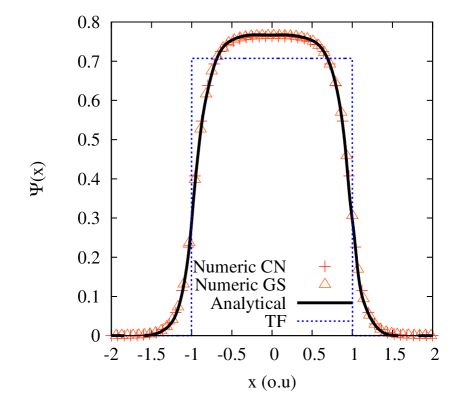
Figure 1: (Color on-line). The computed NLSE ground state wavefunction for a 1-D square-well defect. The ($+$) symbols are the results of the CN method and ($\bigtriangleup$) for the GS method in a square-well with $g_{1}=25$, $V_{0}=50$, and $R_{0}=1.0$ o.u. which gives $\varepsilon_{1}=-35.41668$ o.u.. The analytical wavefunction solution (solid line) of Ref. Carr-LD01-64pra033603 , and the TFA (dashed line) of Eq. (7) are also shown for comparison.

III.3 Determination of $g_{i,max}$

The main computational challenge is to systematically increase $g$ to find $g_{i,max}$ for a given $V_{0}$ and $R_{0}$ for $i=1$-, 2-, and 3-D potentials. Thus, the problem is reduced to a root search for which $\varepsilon_{i}(g_{i,max})=0$ for a given $R_{0}$ and $V_{0}$. As $g_{i}$ is increased, the wavefunction penetrates further into the classically forbidden region, until $g_{i,max}$ is reached, at that point the solution determined is no longer a localized wavefunction Carr-LD01-64pra033603 . To determine $g_{i,max}$ (and hence $N_{max}$) numerically, it is required that the discretized grid be large enough to contain the very slow decay of the wavefunction when $g_{i}$ approaches $g_{i,max}$. Note, however, that we strictly use $\Phi(\pm\bar{x}_{max})=0$, where we effectively have a box $\bar{V}_{1}(\pm\bar{x}_{max})\to\infty$. This means that our $\varepsilon_{i}>0$ scattering states are artificially constrained and are always square integrable.

To ensure that the determined $g_{i,max}$ is accurate to the precision that we demand, the results simply need to be insensitive to the location of the boundary. In our 1-D cases we could simply choose $\bar{x}_{max}=300$ and $\Delta\bar{x}=0.01$. The $g_{i,max}$’s were determined by choosing the defect parameters $V_{0}$ ranging from 0.01, 0.1, 0.5, 1.0, 5.0, 10.0, 20, and 50.0 o.u., while for the width we choose $R_{0}$ from 0.5, 1.0, 2.0, 5.0, 10.0, and 20.0 o.u. commensurate with physical parameters of typical BEC experiments (as discussed later in Sec. IV.5).

For the 2-D cases we chose $\bar{x}_{max}=\bar{y}_{max}=5.0$ in the reduced units space where the potential reaches only unity range and $\Delta\bar{x}=\Delta\bar{y}=0.05$ which gives a 200$\times$200 grid points in the wavefunction. For the 3-D cases, we similarly used $\bar{x}_{max}=\bar{y}_{max}=\bar{z}_{max}=5.0$ and $\Delta\bar{x}=\Delta\bar{y}=\Delta\bar{z}=0.05$ with a wavefunction size of $200\times 200\times 200$. Thus, increasing the dimension in the calculation introduces a large memory footprint, as well as many tri-diagonal matrices to solve in the CN calculations. Compared to the 1-D calculations, we restrict the range of defect parameters explored to ensure accuracy, whilst still spanning the parameter regimes of interest.

In all cases, we assumed convergence for a given $g_{i}$ when $\varepsilon_{i}$ from one iteration to the next changes less than $\Delta\varepsilon_{i}=10^{-8}$. The $g_{i}$ was then incremented until $\varepsilon_{i}=0$ was located to within $10^{-8}$. The amount of increment of $g_{i}$ was 1% of the TFA initial value. When $\varepsilon_{i}>0$ was obtained for a given $g_{i}$, a step back was performed and $\Delta g_{i}$ was reduced in half, until we reached $\varepsilon_{i}=0$ from below.

IV Results and Scaling Laws

IV.1 The 1-D square well case

The numerical and analytical results for the 1-D square well are shown in Table 1 for the smallest and largest value of $R_{0}$ used in this work. The $g_{1,max}$ value was firstly determined for a range of defects spanning large and small values of the product $R_{0}\sqrt{V_{0}}$. We have chosen to translate this into the maximum number of trapped atoms that this corresponds to, specifically for a cloud of ⁸⁷Rb atoms (see caption). These are then compared against the expressions from the TFA, and those obtained by Carr et al. Carr-LD01-64pra033603 and Leboeuf and Pavloff Leboeuf-P01-64pra033602 .

Table 1: The maximum nonlinear coupling constant, $g_{1,max}$, for 1-D square well potentials with various widths ($2R_{0}$) and depths ($V_{0}$) as determined by the 1-D numerical calculations. The corresponding maximum number of atoms trapped by the potentials are given as the $N_{1,max}$ columns assuming that the atomic species is ⁸⁷Rb (with $a_{s}=100a_{0}$, where $a_{0}$ is the Bohr radius) trapped by a transverse frequency of $\omega=2\pi\times 100$ rad/s (thus $a_{\perp}=2.7$ microns). The superscripts denote (a) the numerical calculation, and (b) the present TFA from Eq. (31). The approximations of (c) Carr et al. Carr-LD01-64pra033603 and (d) Leboeuf and Pavloff Leboeuf-P01-64pra033602 are given for comparison.

$R_{0}$	$V_{0}$	$g_{1,max}^{a}$	$N_{1,max}^{a}$	$N_{1,max}^{b}$	$N_{1,max}^{c}$	$N_{1,max}^{d}$
0.5	0.05	0.044346	12.321	13.764	48.597	26.528
0.5	0.1	0.141031	37.003	26.528	73.108	52.056
0.5	0.5	0.852832	218.71	128.64	212.55	256.28
0.5	1	1.635992	418.64	256.28	358.41	511.56
10	0.5	10.679472	2727.3	2553.8	2553.8	5106.6
10	1	21.023785	5368.0	5106.6	5106.6	10212
10	5	102.877445	26264	25529	25529	51057
10	10	204.679689	52252	51057	51057	102113

For large $R_{0}\sqrt{V_{0}}$, the potential is strongly binding and our calculations agree closely with both the TFA and that of Carr et al. Carr-LD01-64pra033603 . In this limit, as we increase the $g_{1}$ towards the $g_{1,max}$ value, the numerical wavefunction resembles the TF wavefunction until we approach extremely close to the $g_{1,max}$ and the wavefunction rapidly delocalizes. Thus, our numerical method for computing $g_{1,max}$ is quite accurate in this regime and not affected by the presence of the boundary conditions. The formula derived by Leboeuf and Pavloff Leboeuf-P01-64pra033602 , with weak binding potentials in mind, has a factor of 2 overestimate in the strong binding limit.

It is also interesting, however, to reconcile the values in Table 1 in the small $R_{0}\sqrt{V_{0}}$ limit. Seaman et al. Seaman-BT05-71pra033609 gives a factor of $g_{1,max}=4\lambda$, the same as the Carr et al. Carr-LD01-64pra033603 in the limit of a small perturbation. That is, the system should approach that of binding to a delta-function of ’strength’ $\lambda=2R_{0}V_{0}$. We expect that our $R_{0}=0.5$, $V_{0}=0.05$ numerical calculation should be close to $g_{1,max}=4\times 2R_{0}V_{0}=0.2$ and not the $g_{1,max}=0.05$ which the TFA estimates. For this weakly bound case we find that, even with our numerical wall located at $\bar{x}_{max}=\pm 300$, our $g_{1,max}$ and thus $N_{1,max}$ are underestimated for the weakest traps. Essentially, the overall energy of the system is artificially raised due to the system being trapped in a finite sized grid, and thus the $g_{1,max}$ needed to reach delocalization is significantly underestimated for small $R_{0}\sqrt{V_{0}}$. Finally, Leboeuf and Pavloff Leboeuf-P01-64pra033602 give a factor of 2 underestimate for small perturbations even though they assumed the limit of a small perturbation in their derivation.

IV.2 The general 1-D trap cases

Figure 2: 1-D scaling law for $g_{1,max}$ weighted by $R_{0}$ for a square (a), circular (b), harmonic (c), double harmonic (d), and triangular well (e) defect, respectively, of various lengths $R_{0}$ and depths $V_{0}$. The numerical results are given as various symbols as indicated in the figure legend, scaled by factors of 10 between each defect shape to avoid nearly overlapping in the figure. The long-dashed lines are a guide for the eye along the numerical results. The TFAs results of Eq. (31) are the solid lines. The square-well results are compared with the analytical expression of Carr et al., Eq. (32), as the short dashed line.

The results for $g_{1,max}$ for all five 1-D defects are shown in Fig. 2 as a function of $R_{0}\sqrt{V_{0}}$. In order to avoid overlapping, the results for the different shape defects have been scaled by a factor of 10 between each other in the ascending order as given by Eq. (31). In the same figure we show the Thomas-Fermi approximations represented by the solid lines, while the long-dashed line is a guide to the eye that follows the numerical results. For the case of the square-well trap, we also show the approximate analytical solution given by Eq. (32) (short-dashed line).

The reason to plot $g_{1,max}R_{0}$ vs. $R_{0}\sqrt{V_{0}}$ in a log-log scale and not $g_{1,max}R_{0}/f(R_{0}\sqrt{V_{0}})$ is to show the range of values that $g_{1,max}$ might take over the range we used in $R_{0}\sqrt{V_{0}}$, and not just to have a constant value defined by the shape factor.

Figure 3: Scaling laws for $g_{1,max}R_{0}/\alpha_{1D}$ as a function of $R_{0}\sqrt{V_{0}}$ for the five different 1-D defect shapes. The solid line is the TFA which becomes identical for all defects. The symbols are the numeric results as obtained from Eq. (33). The short-dashed line is the approximation of Carr et al. Carr-LD01-64pra033603 for the square-well.

As observed in Fig. 2, some symbols are seen to overlap, confirming the basic scaling rule for different widths and depths of the same defect. For large $R_{0}\sqrt{V_{0}}$ the numerical results follow closely the TFA. This is due to large $R_{0}\sqrt{V_{0}}$ which requires a large number of atoms to fill up the defect, i.e., the system is in a strong nonlinearity regime where the TFA is valid. Note though, that this also means that our approximation of holding the wavefunction in a tight transverse state will eventually breakdown. For values of $R_{0}\sqrt{V_{0}}<1$, the kinetic energy term starts to dominate since $g_{1,max}$ gets smaller. It is in this region that the difference between the defect shapes is revealed. However, this is also the region where the 1-D NLSE itself is not valid anymore as mentioned in the introduction.

As the only difference between the 1-D defects is their shape factors [Eq. (34)], we can also plot all of them in a single figure. Figure 3 shows the results by plotting $g_{1,max}R_{0}/\alpha_{1D}$ as a function of $R_{0}\sqrt{V_{0}}$. For $R_{0}\sqrt{V_{0}}>1$ there is barely any difference for all of the trapping defects in the factor $g_{1,max}R_{0}/\alpha_{1D}$, confirming our generalized scaling rule. Thus, under these conditions, the square-well defect holds the most atoms. It is followed by the circular defect, then by the harmonic well defect and the double harmonic well, and finally the triangular defect will hold the least atoms for the same width and depth defects. This is in both the numerical results and the TFA [Eq. (31)].

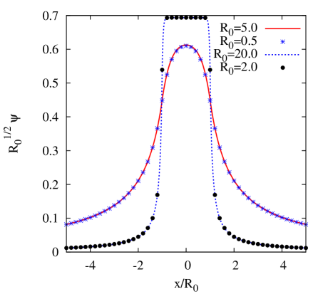
Figure 4: (Color on-line). Scaled 1-D numerical wavefunctions, $\Phi(\bar{x})=\sqrt{R_{0}}\Psi(x/R_{0})$, for various square-well defects. The solid line corresponds to $R_{0}=5.0$ and $V_{0}=0.1$ o.u.; the blue ($*$) symbols correspond to $R_{0}=0.5$ and $V_{0}=10.0$ o.u., such that both of them have the same $R_{0}\sqrt{V_{0}}=1.5811$ and $g_{1,max}R_{0}=6.284$. The dashed line denotes $R_{0}=20.0$ and $V_{0}=0.5$ o.u., while the ($\bullet$) symbol is for $R_{0}=2.0$ and $V_{0}=50.0$ o.u., both of these wavefunctions have $R_{0}\sqrt{V_{0}}=14.1421$ and $g_{1,max}R_{0}=415.770$, thus, showing the same reduced wavefunction.

In Fig. 4, we show the scaled wavefunctions, $\Phi(\bar{x})=\sqrt{R_{0}}\Psi(\bar{x})$, for the square-well defects for two values of $g_{1,max}R_{0}$, and two values of $R_{0}\sqrt{V_{0}}$ as a function of $\bar{x}=x/R_{0}$. The two cases shown give us a small and a large value of $g_{1,max}R_{0}$. For the first case, $R_{0}\sqrt{V_{0}}=1.5811$ and $g_{1,max}R_{0}=6.284$, in particular, the two square-well defect wavefunctions have $R_{0}=5.0$ and $V_{0}=0.1$ o.u. (solid line) for one case, and $R_{0}=0.5$ and $V_{0}=10.0$ o.u. ($*$ symbol) for the other case. That is, a wide and shallow potential trap vs. a tight and deep potential, but both with small $R_{0}\sqrt{V_{0}}$ value.

We note in Fig. 4 that the scaled wavefunction show the same tunneling for both cases of $R_{0}\sqrt{V_{0}}$. However, due to the factor $\sqrt{R_{0}}$ in front of $\Psi$, both cases would have different tunneling in the $x$ oscillator units space. The second case considered in Fig. 4, shows the wavefunction of two square-well defects with $R_{0}\sqrt{V_{0}}=14.1421$ and $g_{1,max}R_{0}=415.770$, in particular, $R_{0}=20.0$ and $V_{0}=0.5$ o.u. (dashed line) and $R_{0}=2.0$ and $V_{0}=50.0$ o.u. ($\bullet$ symbol). Again, we have a wide and shallow potential trap vs. a tight and deep trap, but now with a large values for $R_{0}\sqrt{V_{0}}$. In this case we are in the high $R_{0}\sqrt{V_{0}}$ region where we are closer to the TFA as shown by the shape of the wavefunction which is closer to the potential shape.

The scaling was also verified for the other potentials. In Fig. 5, we show the corresponding scaled wavefunctions for the circular (a), harmonic (b), double harmonic (c) and triangle (d) trap potentials for the same width and depth parameters as those shown in Fig. 4. Note once again how the solutions to the NLSE satisfy the scaling rule, showing the same reduced wavefunction in the reduced units. For the case of the double harmonic trap and the triangle potential trap [Fig. (5c) and (5d)] the wavefunction smooths out for small $g_{1,max}R_{0}$ values in the regions where the potential is non-differentiable in contrast to the strong interaction region where the wavefunction shows the same shape as the trapping potential. Thus, we have confirmed for a given defect that two different shapes with the same $R_{0}\sqrt{V_{0}}$ will have the same $g_{1,max}R_{0}$ and the same reduced wavefunction.

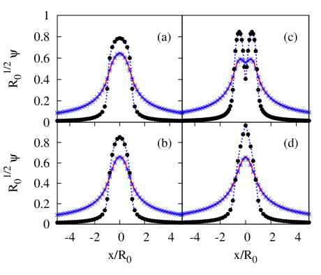
Figure 5: (Color on-line). Scaled 1-D numerical wavefunctions, $\Phi(\bar{x})$, for the (a) circular, (b) harmonic, (c) double harmonic and (d) triangle potential. The labels and parameters are the same as in Fig. 4.

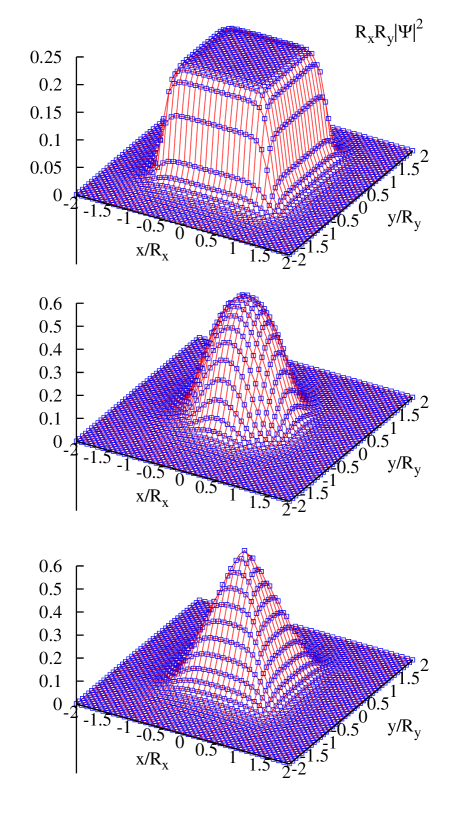
Figure 6: (Color on-line). Numerical scaled density profile solutions, $|\Phi(\bar{x},\bar{y})|^{2}$ for the 2-D NLSE as a function of $\bar{x}$ and $\bar{y}$ for the square, parabolic, and pyramid trap defects for $V_{0}=50.0$ and $R_{x}=R_{y}=R_{0}=1.0$ o.u. for the solid lines (red lines). In the same figure we show the results for $V_{0}=2.0$ and $R_{x}=R_{y}=R_{0}=5.0$ o.u. represented by the squared symbols (blue), thus confirming the scaling density profile rule for the 2-D case.

IV.3 The 2-D trap cases

For the two-dimensional cases we show in Fig. 6 the probability density for the three potential cases (square, harmonic, and pyramid well potentials). In these cases we show the results for $R_{x}=R_{y}=R_{0}=1.0$ o.u. and $V_{0}=50.0$ o.u. for the results in red lines (solid lines). Interestingly, the wavefunction takes a shape similar to the potential the particles are being held, in the same way as the 1-D case. In the same figure, we show the results for $R_{x}=R_{y}=R_{0}=5.0$ o.u. and $V_{0}=2.0$ o.u. for the results shown by the symbols (blue squares). Both cases have $R_{0}\sqrt{V_{0}}=7.071$, therefore both of them have the same scaled wavefunction, $\Phi=\sqrt{R_{x}R_{y}}\Psi=R_{0}\Psi$, confirming our scaling rule, i.e. the same reduced density profile.

In Fig. 7, we show the ratio of the nonlinear coupling term $g_{2,max}$ to the shape form factor $\alpha_{2D}$ for the 2-D results as a function of $R_{0}\sqrt{V_{0}}$. The solid lines are the Thomas-Fermi results and the symbols are the data obtained by our numerical procedure. Again, for $R_{0}\sqrt{V_{0}}>10$ the Thomas-Fermi results follow closely the numerical data for $g_{2,max}/\alpha_{2D}$ showing a universal behavior for the non-linear coupling term. Discrepancies start to appear in the results for small values of $R_{0}\sqrt{V_{0}}$, dependent of the defect shape. This is a consequence of the neglect of the kinetic energy term in the TFA, and thus the neglect of tunneling for these weakly bound particles.

Figure 7: Scaling law for the 2-D defects, $g_{2,max}/\alpha_{2D}$ of the nonlinear coupling constant as a function of $R_{0}\sqrt{V_{0}}$ for the square, parabolic, and pyramid trapping potential for the 2-D NLSE. The solid line is the Thomas-Fermi result. Symbols are our numerical results at the threshold of delocalization. The upper/middle/lower symbols are, respectively, for square, parabolic and pyramid shaped defects.

IV.4 The 3-D trap cases

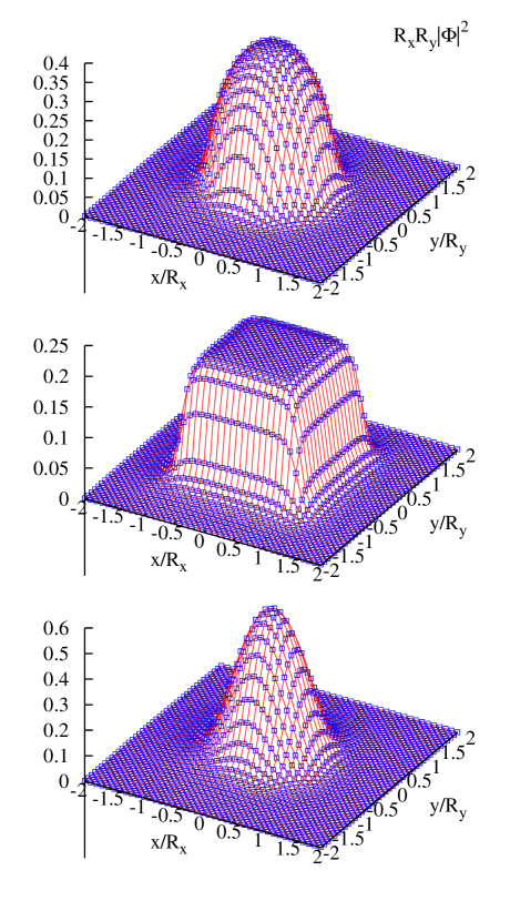
Figure 8: (Color on-line). Numerical projected scaled density profile solutions, $|\Phi(\bar{x},\bar{y})|^{2}$ to the 3-D NLSE as a function of $x$ and $y$ for the spherical, rectangular cuboid, and parabolic well trap potentials for $R_{x}=R_{y}=R_{z}=1.0$ o.u. and $V_{0}=50.0$ for the solid lines (red lines). In the same figure we show the results for $R_{x}=R_{y}=R_{z}=2.0$ o.u. and $V_{0}=5.0$ by the squared symbols (blue), thus confirming the scaling density profile rule for the 3-D case.

In order to visualize the density profile of a 3-D wavefunction, we project the reduced wavefunction onto the $z$-axis such that

$$|\Phi(\bar{x},\bar{y})|^{2}=\int|\Phi(\bar{x},\bar{y},\bar{z})|^{2}d\bar{z}\,.$$ (60)

Thus, for the three-dimensional case, we show in Fig. 8 the projected scaled density profiles, $|\Phi(\bar{x},\bar{y})|^{2}$, for the spherical, rectangular cuboid and harmonic well potentials. For these two cases we show the results for $R_{x}=R_{y}=R_{0}=1.0$ o.u. and $V_{0}=50.0$ o.u.. The wavefunction takes a shape similar to the defect that the particles are being held, as the 1- and 2-D wavefunctions also tended to do. In the same figure, we show the results for $R_{x}=R_{y}=R_{0}=5.0$ o.u. and $V_{0}=2.0$ o.u.. Both cases have $R_{0}\sqrt{V_{0}}=7.071$, and therefore have the same scaled wavefunction $\Phi=\sqrt{R_{x}R_{y}R_{z}}\Psi=R_{0}^{3/2}\Psi$, as well as the same $g_{3,max}/R_{0}$ confirming that our scaling rule further holds in 3-D.

In Fig. 9, we show the ratio of the nonlinear coupling term $g_{3,max}$ to the shape form factor $\alpha_{3D}$ for the three dimensional results as a function of $R_{0}\sqrt{V_{0}}$. The solid straight line is the Thomas-Fermi results and together with the symbols are the data obtained by our numerical procedure. Again, for $R_{0}\sqrt{V_{0}}>10$ the Thomas-Fermi results follow closely the numerical data for $g_{3,max}/\alpha_{3D}R_{0}$ showing an universal behavior for the non-linear coupling constant. For small values of $R_{0}\sqrt{V_{0}}$, discrepancies, dependent of the potential trap shape, start to appear in the results consequence of the kinetic energy term. In the same figure, we show the variational results for Adhikari Adhikari-SK07-42ejpd279 . As mentioned in the introduction, his results overestimates the TFA or our numerical results.

Figure 9: Scaling law of the 3-D nonlinear coupling constant divided by the potential shape factor $\alpha_{3D}$ as a function of $R_{0}\sqrt{V_{0}}$ for the spherical, rectangular cuboid, and parabolic trapping potential for the 3-D NLSE. The solid line is the Thomas-Fermi result. The symbols are our numerical results near delocalization. The upper/middle/lower symbols are, respectively, for spherical, rectangular cuboid, and parabolic shaped defects. The dashed line represents the variational results from Adhikari Adhikari-SK07-42ejpd279 for the spherical well.

IV.5 Application: A 3-D cube trap

The application and implications of this work follows directly from the scaling law for the non-linear coupling constant and the reduced density profile for the 1-, 2-, and 3-D cases considered. The NLSE in physical units is Dalfovo-F99-71rmp463

$$\left\{-\frac{\hbar^{2}}{2m}\nabla^{2}+V_{trap}(\mathbf{r})\right. +$$ (61)

$$\left.\frac{4\pi\hbar^{2}a_{s}(N-1)}{m}|\Psi_{0}(\mathbf{r})|^{2}\right\}\Psi_{0}(\mathbf{r}) = \varepsilon_{0}\Psi_{0}(\mathbf{r}).$$

For a trap with characteristic harmonic oscillator lengths $l_{x}$, $l_{y}$, and $l_{z}$ for each Cartesian coordinate, such that a transformation to oscillator units requires $\mathbf{r}=(l_{x}l_{y}l_{z})^{1/3}\bar{\mathbf{r}}$, and the NLSE in o.u. becomes

$$\left\{-\frac{1}{2}\bar{\nabla}^{2}+\bar{V}_{trap}(\bar{\mathbf{r}})+g_{3}|\Psi(\bar{\mathbf{r}})|^{2}\right\}\Psi(\bar{\mathbf{r}})=\varepsilon\Psi(\bar{\mathbf{r}})$$ (62)

where

$$g_{3} = \frac{4\pi a_{s}(N-1)}{(l_{x}l_{y}l_{z})^{1/3}}$$ (63)

$$V = \frac{m(l_{x}l_{y}l_{z})^{2/3}}{\hbar^{2}}V_{3}^{\prime}$$ (64)

$$\varepsilon = \frac{m(l_{x}l_{y}l_{z})^{2/3}}{\hbar^{2}}\varepsilon_{0}$$ (65)

As an example we again choose ⁸⁷Rb atoms with $a_{s}=100\,a_{0}$ as in the experiment of Ref. Anderson-MH95-269science198 . We consider the trap as a 3-D cube with length scale $l_{x}=l_{y}=l_{z}=1.222\times 10^{-4}$ cm $=23000a_{0}$ and thus a volume of $8\times l_{x}^{3}$. The TFA then gives us $g_{3}=0.05464(N-1)$ and $V=2.68\times 10^{8}$ $V_{trap}$(o.u/$K$), where the potential trap depth is given in units of absolute temperature (Kelvin). Thus, for $R_{0}$ covering the range from $1$ to $10$ o.u., as used in Sec. IV.4 with physical values that correspond to a BEC with extension between $1.22$ and $12.2$ $\mu$m. Similarly, for $V=V_{0}$ covering the range from $1$ to $50$ o.u. this is equivalent to traps depths of $3$ to $150$ nK, which are values well within the range of the experiment. The values reported in Fig 9 thus correspond to a range from $200$ to $2\times 10^{6}$ atoms, which are typically found in experiments.

V Conclusions

In conclusion, by means of the Thomas-Fermi approximation at the delocalization threshold, $\varepsilon_{i}=0$, one can easily determine an approximation to the maximum non-linear interaction strength $g_{i,max}$ of the Gross-Pitaevskii equation and therefore, the maximum number of atoms, $N_{max}$, that can be trapped by $i=$1-, 2-, and 3-D potentials that contain a defect.

The scaling laws of Eqs. (31), (43), and (52) are dependent on both the depth and length of the potential, and remain valid over a surprisingly wide-range of parameters. The TFA relies on a wavefunction that is constrained by the shape of the potential, never diffusing into the classically forbidden region. At the $g_{i,max}$ point the TF wavefunction becomes unbound, and that this mimics the actual solution to the NLSE which diffuses towards infinity as $g_{i}$ approaches $g_{i,max}$ is remarkable. It would, however, be worthwhile to extend this work through a more sophisticated variational treatment Carretero-Gonzalez-R08-21nljR139 .

The existence of these scaling laws is useful because it captures in a simple expression the number of atoms of a BEC that can be trapped by a potential defect on waveguide or in free-space. It would be interesting to further examine the dynamic scattering/trapping of a BEC as it propagates through such defects Ernst-T10-81pra033614 ; Gattobigio-GL10-12njp085013 . Essentially, the non-linear term enables a continuum of non-linear bound states, as opposed to the quantized single-particle eigenstates. For example, if $N_{max}=200$ atoms, then any number lower than that will also be able to be trapped. How easy is it for a BEC with $N>N_{max}$ to fill up the defect as it goes past remains to be demonstrated, and our initial calculations within the NLSE show very little, if any, filling up of the defect. It will also be interesting to consider that the presence of any localized atoms will tend to smooth out the defect potential that a consequent BEC interacting with the defect will experience. This may have an impact, e.g. on Anderson-type localization.

References

- (1) M. H. Anderson, J. R. Ensher, M. R. Matthews, C. E. Wieman, and E. A. Cornell, Science 269, 198 (July 1995)
- (2) K. B. Davis, M. O. Mewes, M. R. Andrews, N. J. van Druten, D. S. Durfee, D. M. Kurn, and W. Ketterle, Phys. Rev. Lett. 75, 3969 (Nov 1995)
- (3) Bose-Einstein Condensation, edited by A. Griffin, D. Snoke, and S. Stringaro (Cambridge University Press, New York, 1995)
- (4) A. S. Parkins and D. F. Walls, Physics Reports 303, 1 (1998), ISSN 0370-1573, http://www.sciencedirect.com/science/article/pii/S0370157398000143
- (5) F. Dalfovo, S. Giorgini, L. P. Pitaevskii, and S. Stringari, Rev. Mod. Phys. 71, 463 (Apr 1999)
- (6) J. Fortágh and C. Zimmermann, Rev. Mod. Phys. 79, 235 (Feb 2007)
- (7) A. D. Cronin, J. Schmiedmayer, and D. E. Pritchard, Rev. Mod. Phys. 81, 1051 (Jul 2009)
- (8) A. E. Leanhardt, A. P. Chikkatur, D. Kielpinski, Y. Shin, T. L. Gustavson, W. Ketterle, and D. E. Pritchard, Phys. Rev. Lett. 89, 040401 (Jul 2002)
- (9) S. K. Schnelle, E. D. van Ooijen, M. J. Davis, N. R. Heckenberg, and H. Rubinsztein-Dunlop, Opt. Express 16, 1405 (Feb 2008)
- (10) K. Henderson, C. Ryu, C. MacCormick, and M. G. Boshier, New Journal of Physics 11, 043030 (2009), http://stacks.iop.org/1367-2630/11/i=4/a=043030
- (11) B. D. Esry, Phys. Rev. A 55, 1147 (1997)
- (12) M. Jääskeläinen and S. Stenholm, Phys. Rev. A 66, 023608 (Aug 2002)
- (13) T. Lahaye, P. Cren, C. Roos, and D. Guéry-Odelin, Communications in Nonlinear Science and Numerical Simulation 8, 315 (2003), ISSN 1007-5704, chaotic transport and compexity in classical and quantum dynamics, http://www.sciencedirect.com/science/article/pii/S1007570403000327
- (14) P. Leboeuf, N. Pavloff, and S. Sinha, Phys. Rev. A 68, 063608 (Dec 2003)
- (15) M. Koehler, M. W. J. Bromley, and B. D. Esry, Phys. Rev. A 72, 023603 (Aug 2005)
- (16) P. Leboeuf and N. Pavloff, Phys. Rev. A 64, 033602 (Aug 2001)
- (17) M. W. J. Bromley and B. D. Esry, Phys. Rev. A 68, 043609 (2003)
- (18) M. W. J. Bromley and B. D. Esry, Phys. Rev. A 69, 053620 (May 2004)
- (19) T. Ernst and J. Brand, Phys. Rev. A 81, 033614 (Mar 2010)
- (20) G. L. Gattobigio, A. Couvert, B. Georgeot, and D. Guéry-Odelin, New Journal of Physics 12, 085013 (2010), http://stacks.iop.org/1367-2630/12/i=8/a=085013
- (21) M. W. J. Bromley and B. D. Esry, Phys. Rev. A 70, 013605 (2004)
- (22) L. D. Carr, K. W. Mahmud, and W. P. Reinhardt, Phys. Rev. A 64, 033603 (Aug 2001)
- (23) B. T. Seaman, L. D. Carr, and M. J. Holland, Phys. Rev. A 71, 033609 (Mar 2005)
- (24) S. K. Adhikari, The European Physical Journal D - Atomic, Molecular, Optical and Plasma Physics 42, 279 (2007), ISSN 1434-6060, 10.1140/epjd/e2007-00006-0, http://dx.doi.org/10.1140/epjd/e2007-00006-0
- (25) J. A. López-Miranda, R. Cabrera-Trujillo, M. W. J. Bromley, and B. D. Esry, ICPIG conference proceedings XXIX, PA1.3 (2009)
- (26) M. Edwards and K. Burnett, Phys. Rev. A 51, 1382 (Feb 1995)
- (27) G. Baym and C. J. Pethick, Phys. Rev. Lett. 76, 6 (Jan 1996)
- (28) J. Crank and P. Nicolson, Proc. Cambridge Phil. Soc. 43, 50 (1947)
- (29) W. H. Press, S. A. Teukolsky, W. T.Vetterling, and B. P. Flannery, Numerical recipes, 2nd ed. (Cambridge University Press, New York, USA, 1992) ISBN 052143064X
- (30) A. Goldberg, H. M. Schey, and J. L. Schwartz, Am. J. Phy. 35, 177 (1967), http://dx.doi.org/10.1119/1.1973991
- (31) B. D. Esry, C. H. Greene, J. P. Burke Jr., and J. L. Bohn, Phys. Rev. Lett. 78, 3594 (1997)
- (32) S. E. Kooning and D. C. Meredith, Computational Physics, FORTRAN version (Perseus Books, Reading, MA, USA, 1990)
- (33) R. Carretero-González, D. J. Frantzeskakis, and P. G. Kevrekidis, Nonlinearity 21, R139 (2008), http://stacks.iop.org/0951-7715/21/i=7/a=R01