Freezing Transition, Characteristic Polynomials of Random Matrices,                                            and the Riemann Zeta-Function

Abstract

We argue that the freezing transition scenario, previously explored in the statistical mechanics of $1/f-$noise random energy models, also determines the value distribution of the maximum of the modulus of the characteristic polynomials of large $N\times N$ random unitary (CUE) matrices. We postulate that our results extend to the extreme values taken by the Riemann zeta-function $\zeta(s)$ over sections of the critical line $s=1/2+it$ of constant length and present the results of numerical computations in support. Our main purpose is to draw attention to possible connections between the statistical mechanics of random energy landscapes, random matrix theory, and the theory of the Riemann zeta function.

The Riemann zeta-function

$$\zeta(s)=\sum_{n=1}^{\infty}\frac{1}{n^{s}}=\prod_{p}\left(1-\frac{1}{p^{s}}\right)^{-1}$$ (1)

encodes the distribution of the primes $p$ in the positions of its non-trivial zeros Titchmarsh . The Riemann Hypothesis, which is of central importance in mathematics, places these zeros on the critical line $s=1/2+it,\,t\in\mathbb{R}$. There has in recent years been considerable interest, stemming from speculations about a spectral interpretation of the Riemann zeros, in possible connections between the theory of the zeta-function and quantum mechanics (see, e.g. qm ). Our focus here is on suggesting a new link with physics via the statistical mechanics of disordered landscapes.

Some of the most significant questions in the theory of the zeta function concern the distribution of values it takes on the critical line, where it behaves like a quasi-random function of $t$ (essentially because the phases of the terms in the product in (1) contribute as if they were random) . It was proved by Selberg, for example, that, as $t\rightarrow\infty$, $\log|\zeta(1/2+it)|$ behaves like a Gaussian random variable with mean zero and variance $\frac{1}{2}\log\log\frac{t}{2\pi}$, see e.g. Lau . In other words, the typical size of $\log|\zeta(1/2+it)|$ is of the order of $\sqrt{\log\log t}$. As regards the extreme values taken by the zeta function over long ranges, the Lindelöf Hypothesis asserts that $|\zeta(1/2+it)|$ grows more slowly than any power of $t$ as $t\rightarrow\infty$, the Riemann Hypothesis implies that it is $O(\exp({\rm const.}f(t)))$, where $f(t)=\log t/\log\log t$, while it is known that $|\zeta(1/2+it)|$ takes values at least as large as $\exp(\sqrt{f(t)})$ infinitely often (Titchmarsh, , pp. 354, 209). The extreme values thus lie in the range between these upper and lower bounds (and are significantly larger than the typical values). The problem of determining where precisely within this range they lie has attracted considerable attention, but remains unresolved. The extreme values in question are so rare that numerical computations have failed to settle the matter so far.

One model, proposed by Montgomery, that leads to predictions for the extreme values is based on the assumption that the local maxima of $\log|\zeta(1/2+it)|$ are statistically independent and that they obey the normal distribution proved for general values. Under such assumptions one finds that the typical size of the maximum value of $|\zeta(1/2+it)|$ should be of the order of $\exp\left(c_{M}\sqrt{\log(t)\log\log(t)}\right)$ FGH , where $c_{M}$ is a constant. This is closer to the lower bound than the upper bound, implying that the extreme values are not much larger than the largest value known to be reached infinitely often.

However, the values of $\log|\zeta(1/2+it)|$ are, in fact, strongly correlated in a way that is significant from the point of view we shall explore here. Specifically, define, for a fixed $t\in\mathbb{R}$,

$$V_{t}^{(\zeta)}(x)=-2\log{|\zeta\left(\frac{1}{2}+i(t+x)\right)|}$$ (2)

Selberg’s theorem implies that $V_{t}^{(\zeta)}(x)$ behaves like a Gaussian random function of $x$ when $t\to\infty$. Such a random process is characterized by the two-point correlation function $C(x_{1},x_{2})=\overline{V^{(\zeta)}_{t}(x_{1})V^{(\zeta)}_{t}(x_{2})}$, with the bar denoting the average over intervals $[t-h/2,t+h/2]$, with $h\ll t$ chosen so that the intervals contain, asymptotically (as $t\to\infty$), an increasing number of zeros. A straightforward calculation, sketched in FyoKeat , see also Bourg , leads to

$$C(x_{1},x_{2})=\left\{\begin{array}[]{c}-2\log{|x_{1}-x_{2}|},\,\,\mbox{for}\quad\frac{1}{\log{t}}\ll|x_{1}-x_{2}|\ll 1\\ 2\log{\log{t}},\,\,\mbox{for}\quad|x_{1}-x_{2}|\ll\frac{1}{\log{t}}\end{array}\right.$$ (3)

The significance of the logarithmic form of the correlations will become apparent when we come to make comparisons with corresponding problems in random matrix theory and statistical mechanics.

Over the past 40 years, inspired by the pioneering work of Montgomery Montpair and Odlyzko Odl , considerable evidence has accumulated for connections between the statistical properties of the Riemann zeta-function and those of large random matrices. For example, correlations between the nontrivial zeros of the zeta function are believed to coincide asymptotically with those between the eigenvalues of large random unitary or hermitian matrices Montpair ; Odl , and the value distribution of $\zeta(1/2+it)$ is believed to be related to that of the characteristic polynomials of these matrices KeatSna00 ; HKO ; CFKMS ; GHK . Our purpose here is to connect these two areas of research to a third, the statistical mechanics of disordered logarithmically-correlated energy landscapes, see CLD ; FB ; FLDR and references therein. The analogy we develop suggests that the spin-glass-like freezing transition that dominates the low-temperature behaviour in the statistical mechanical problems also governs the extreme values taken by the characteristic polynomials of random matrices and the zeta function. This sheds new light on the longstanding problem of determining the maximum size of $\zeta(1/2+it)$.

To establish such a connection we consider the ensemble of $N\times N$ unitary matrices, chosen uniformly at random from the unitary group ${\cal U}(N)$ (i.e. from the Circular Unitary Ensemble, or CUE). We denote the eigenvalues of a given matrix $U_{N}$ by $\exp{(i\phi_{1})},\ldots,\exp{(i\phi_{N})}$ and the corresponding characteristic polynomial by

$$p_{N}(\theta)=\det{\left(1-U_{N}\,e^{-i\theta}\right)}=\prod_{n=1}^{N}\left(1-e^{-i(\phi_{n}-\theta)}\right).$$ (4)

It is instructive to compare $V_{t}^{(\zeta)}(x)$ from (2) with $V^{(U)}_{N}(\theta)=-2\log{|p_{N}(\theta)|}$. It was proved in KeatSna00 that $V^{(U)}_{N}(\theta)$ satisfies a central limit theorem: the distribution of the values of $\log|p_{N}(\theta)|$ tends to a normal with mean zero and variance $2\log{N}$ as $N\rightarrow\infty$. Identifying the mean density of the eigenvalues, $N/2\pi$, with the mean density of the Riemann zeros near to height $t$, $\frac{1}{2\pi}\log\frac{t}{2\pi}$, renders the agreement with Selberg’s theorem for $\log|\zeta(1/2+it)|$ complete. Importantly for us here, $V^{(U)}_{N}$ has the following representation HKO :

$$V^{(U)}_{N}(\theta)=\sum_{n=1}^{\infty}\frac{1}{\sqrt{n}}\left[e^{-in\theta}v^{(N)}_{n}+\mbox{comp. conj.}\right]$$ (5)

with $\sqrt{n}v^{(N)}_{n}=\mbox{Tr}\left(U_{N}^{-n}\right))$. According to DiaSha , as $U_{N}$ varies in the CUE the coefficients $v^{(N)}_{n}$ for any fixed $n$ tend in the limit $N\to\infty$ to independent, identically distributed complex gaussian variables with zero mean and unit variance. Denoting averages over the unitary group ${\cal U}(N)$ with the angular brackets, a simple calculation shows that $\left\langle V^{(U)}_{N}(\theta_{1})V^{(U)}_{N}(\theta_{2})\right\rangle$ tends in the limit $N\to\infty$ to $-2\log\left(2|\sin\frac{1}{2}(\theta_{1}-\theta_{2})|\right)$, and so exhibits precisely the same logarithmic behaviour at small distances as in (3). For large but finite $N$, the logarithmic divergence can be shown to saturate at $|\theta_{1}-\theta_{2}|\sim N^{-1}$, so after associating $N\sim\log\frac{t}{2\pi}$ the correspondence between the small-scale behaviour of $V^{(U)}_{N}(\theta)$ and $V_{t}^{(\zeta)}(x)$ becomes complete. This is significant from the point of view we seek to develop.

Our primary goal is to determine the distribution of the maximum value of $|p_{N}(\theta)|$ over $0\leq\theta\leq 2\pi$ when the matrix $U_{N}$ ranges over ${\cal U}(N)$. Our second goal is then to use the random-matrix results to motivate predictions for the extreme values of the Riemann zeta function. The first steps in this direction were taken in FGH , where the tail of the distribution of the maximum values of $|p_{N}(\theta)|$ in $0\leq\theta\leq 2\pi$ was found. This tail determines the typical size of the maximum values expected when $U_{N}$ is sampled independently a large (exponentially in $N$) number of times from within ${\cal U}(N)$. The results are consistent with the Montgomery model and lead to a prediction for the value of the constant $c_{M}$ there.

The focus here will differ from that of FGH in the following ways. We shall be concerned with the distribution of maximum values of the characteristic polynomials of single matrices, rather than with large numbers of matrices, and will obtain the full value distribution of the maxima in the limit as $N\rightarrow\infty$, rather than concentrating on the tail that is relevant when maximizing over many matrices. This leads to a model for the distribution of maximum values of $|\zeta(1/2+it)|$ over the intervals $T\leq t\leq T+2\pi$, rather than $0\leq t\leq T$ as $T\rightarrow\infty$. Furthermore, it makes the problem of numerical computation of the distribution in question significantly easier, because one is finding the maximum of $\sim\log T$ rather than $\sim T\log T$ numbers (the values of the local maxima).

We start by noting that the maximum value of $p_{N}(\theta)$ can be characterized in terms of

$${\cal Z}_{N}(\beta)=\frac{N}{2\pi}\int_{0}^{2\pi}|p_{N}(\theta)|^{2\beta}d\theta\equiv\frac{N}{2\pi}\int_{0}^{2\pi}e^{-\beta V_{N}(\theta)}\,d\theta,$$ (6)

where $V_{N}(\theta)=-2\log{|p_{N}(\theta)|}$ and $\beta>0$. Specifically, if ${\cal F}(\beta)=-\beta^{-1}\log{{\cal Z}_{N}(\beta)}$, then

$$\lim_{\beta\to\infty}{\cal F}(\beta)=\min_{\theta\in(0,2\pi)}V_{N}(\theta)=-2\max_{\theta\in(0,2\pi)}\log{|p_{N}(\theta)|}.$$ (7)

The key observation is that (6) takes the form of the partition function for a system with energy $V_{N}(\theta)$ and inverse temperature $\beta$. ${\cal F}(\beta)$ may then be associated with the corresponding free energy. Recalling that the values of $V_{N}(\theta)$ are asymptotically gaussian distributed and logarithmically correlated, it is natural to draw comparisons with a class of problems that has attracted a good deal of attention recently in the area of disordered systems, namely the statistical mechanics of a particle equilibrated in a random landscape with logarithmic correlations. Two-dimensional systems of that sort appear in many contexts, for example in the problem of Dirac fermions in a random magnetic field CMW , and one-dimensional analogues were considered recently in FB ; FLDR . Importantly for us, in the one-dimensional case the energy landscape is given by a regularization of the random Fourier series featuring in (5). In the statistical mechanical problem there has been a particular focus on the so-called freezing transition CMW ; CLD which dominates the low temperature limit and determines the extreme value statistics. The latter appears to be manifestly different from the case of uncorrelated variables. We shall argue that a similar freezing transition determines the extreme value statistics of the characteristic polynomials and hence, conjecturally, of $|\zeta(1/2+it)|$, and that therefore the logarithmic correlations exhibited by $V^{(U)}_{N}(\theta)$ and $V_{t}^{(\zeta)}(x)$ play an important role.

The first step is to consider the positive integer moments $\left\langle{\cal Z}_{N}^{k}(\beta)\right\rangle,\quad k=1,2,\ldots$. Using standard methods of random matrix theory (RMT) it is easy to show that

$$\left\langle{\cal Z}_{N}^{k}(\beta)\right\rangle=N^{k}\int_{0}^{2\pi}\ldots\int_{0}^{2\pi} \frac{D_{N}^{(k)}(\beta)}{D_{N}^{(k)}(0)}\prod_{j=1}^{k}\frac{d\theta_{j}}{2\pi},\,$$ (8)

where $D_{N}^{(k)}(\beta)=\det{\left(M_{i-j}^{(\beta)}\right)_{i,j=0}^{N-1}}$ is the determinant of a Toeplitz matrix

$$M_{i-j}^{(\beta)}=\int_{0}^{2\pi}e^{i\phi(i-j)}\prod_{p=1}^{k}\left[2-2\cos{(\phi-\theta_{p})}\right]^{\beta}\frac{d\phi}{2\pi}\,.$$ (9)

When $N\to\infty$ the asymptotics of such Toeplitz determinants is well known Wid to be given by

$$D_{N}^{(k)}\approx\left[N^{\beta^{2}}\frac{G^{2}(1+\beta)}{G(1+2\beta)}\right]^{k}\prod_{r<s}^{k}|e^{i\theta_{r}}-e^{i\theta_{s}}|^{-2\beta^{2}}\,,$$ (10)

where $G(x)$ is the so-called Barnes function. Substituting (10) back to (8) we see that the resulting expression is the standard Dyson-Morris version of the Selberg integral FWSel , convergent for $k<\frac{1}{\beta^{2}}$, and divergent for larger $k$. As we have $k\geq 1$ the procedure makes sense only for $\beta^{2}~{}<~{}1$. Introducing ${\cal Z}_{e}=N^{1+\beta^{2}}\frac{G^{2}(1+\beta)}{G(1+2\beta)\Gamma(1-\beta^{2})}$, we find

$$\left\langle{\cal Z}_{N}^{k}(\beta)\right\rangle={\cal Z}_{e}^{k}\Gamma(1-k\beta^{2}),\quad k<\beta^{-2}\,.$$ (11)

The expression (11) for the moments has exactly the same form as that for the partition function of the landscape of the circular-logarithmic model (a periodic version of $1/f$ noise) FB , but with a different value for the characteristic scale ${\cal Z}_{e}$. This means we can simply translate, mutatis mutandis, the results of FB to the values of characteristic polynomial sampled along the full circle $\theta\in(0,2\pi]$. In particular, we conclude that the maximum value of the modulus of a CUE characteristic polynomial $p_{N}(\theta)$ in an interval $\theta\in[0,2\pi]$ can be written in the limit $N\rightarrow\infty$ as

$$-2\max_{\theta\in[0,2\pi)}{\log{|p_{N}(\theta)|}}\sim a_{N}+b_{N}\,x,$$ (12)

where $a_{N}=-2\log{N}+c\log{\log{N}}+o(1)$, with, conjecturally, $c=\frac{3}{2}$, $b_{N}=1+O(1/\log{N})$, and $x$ is a random variable taking values distributed with probability density

$$p(x)=2e^{x}K_{0}(2e^{x/2}),$$ (13)

where $K_{\nu}(z)$ denotes the modified Bessel function. Two consequences are particularly noteworthy: (i) the tail of the probability density of the random variable $x$ is given asymptotically when $x\to-\infty$ by $p(x)\sim|x|e^{x}$, (ii) the value of the constant $c=3/2$. These two features are believed to be universal characteristics of the extreme value statistics of the class of logarithmically correlated random variables CLD , and distinguish those from short-range correlated random variables, for which $c=1/2$ and $p(x)\sim e^{x}$ (Gumbel distribution) LLR . This new class is believed to include, in particular, the $2D$ Gaussian free field BZ , branching random walks ABK , polymers on disordered trees DS , $1/f$ noise FB ; FLDR and models appearing in turbulence and financial mathematics turbfin .

In order to illustrate the extreme value predictions in the context of the Riemann zeta function we now summarize the results of preliminary numerical computations. These involved numerically evaluating $\zeta(1/2+it)$ over ranges of length $2\pi$, at various heights $T$, and finding the maximum value $\zeta_{\rm max}(2\pi;T)$ in each range. We used the amortized-complexity algorithm Hia , which is suitable for computing $\zeta(1/2+it)$ at many points.

The first test concerns the value of the constant $c$ in (12). We expect the logarithmic correlations to lead to $c=\frac{3}{2}$, rather than $c=\frac{1}{2}$, as would be the case if the zeta correlations were short-range. The mean of $\zeta_{\rm max}(2\pi;T)$ suggested by the model in (12) is $\delta=e^{\gamma}N/(\log N)^{\frac{c}{2}}$, with $c=1/2\textrm{ or }3/2\,,$ and $\gamma=0.57721\ldots\,,$ where we set $N$ to be the nearest integer to $\log T$. At each height a sample that spans $\approx 10^{7}$ zeros is used yielding $\approx 10^{7}/N$ sample points (since there are roughly $N$ zeros in each range of length $2\pi$). In view of the table below, one may conclude that $c=3/2$ fits the data considerably better than $c=1/2$, thus supporting the logarithmic correlations model.

Table 1: Ratio of data mean $\tilde{\delta}$ to model mean $\delta$ with $c=3/2$ and $c=1/2$.

$T$	$\qquad N\qquad$	$\left(\tilde{\delta}/\delta\right)_{c=3/2}$	$\left(\tilde{\delta}/\delta\right)_{c=1/2}$
$10^{22}$	51	1.001343	0.504993
$10^{19}$	44	0.992672	0.510293
$10^{15}$	35	0.976830	0.518057
$3.6\times 10^{7}$	17	0.930533	0.552856

Testing the distribution $p(x)$ is more difficult, because the data converge extremely slowly at that scale. The results of our initial experiments are summarized in Figure 1. Specifically, we consider $-2\log|\zeta_{\rm max}(2\pi;T)|+2\log N-\frac{3}{2}\log\log N$ based on a set of approximately $2.5\times 10^{8}$ zeros near $T=10^{28}$. The data are normalized so that $-2\log|\zeta_{\rm max}(2\pi;T)|+2\log N-\frac{3}{2}\log\log N$ has empirical variance $=\int x^{2}p(x)\,dx=3.28986813\ldots$. The overall agreement is supportive of (13), especially in the important tail when $x\to-\infty$ and in view of the fact that lower order arithmetical terms KeatSna00 ; CFKMS have not been incorporated, but cannot be said to be a conclusive verification at this stage. The behaviour in the tail is significant because if it were to persist into the large deviation regime it would suggest that the Montgomery heuristic significantly underestimates the maximum values achieved by $|\zeta(1/2+it)|$, although this seems unlikely.

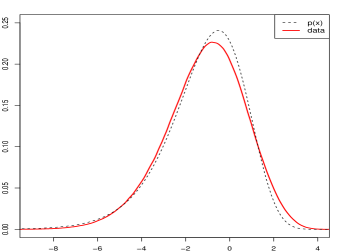
Figure 1: Numerical computation (solid red line) compared to theoretical prediction (13) (dashed black line) for $p(x)$.

Finally, we put the specific idea of the freezing to a numerical test by considering the analogue of the partition function ${\cal Z}_{N}(\beta)$ defined by (6) which is clearly

$$z_{\beta}(T)=\frac{N_{T}}{2\pi}\int_{T}^{T+2\pi}|\zeta(1/2+iy)|^{2\beta}dy,$$ (14)

where $N_{T}=\log\frac{T}{2\pi}$, and calculating the ensuing free energy $f(\beta)=-(\beta\log{(N_{T})})^{-1}\overline{\log{z_{\beta}}}$ by averaging over $10^{6}$ values of $T$ near $T=10^{28}$. If freezing is operative, -$f(\beta)$ is expected to be equal to $\beta+1/\beta$ for $\beta<\beta_{c}=1$ and remain frozen to $-f(\beta)=2$ for all $\beta>1$ CLD ; FB ; FLDR . The results shown in Figure 2 (which are renormalized by the subtraction of lower order arithmetic terms FyoKeat ) again are consistent with this prediction.

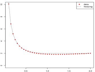
Figure 2: Numerical computation (red dots) compared to the theoretical prediction (dashed black line) for $-f(\beta)$, suggesting freezing beyond $\beta=1$

To conclude, we have put forward speculations on the existence and implications of the freezing phenomena seen in the statistical mechanics of random energy landscape models in the context of the extreme value distribution of the characteristic polynomials of large random matrices and, further, of the Riemann zeta-function on the critical line. We believe this sheds interesting new light on these problems. In a forthcoming paper FyoKeat we present the details of our calculations and discuss further the broader picture of freezing phenomena and their manifestation in the present context.

Support by the EPSRC grant EP/J002763/1 (YVF), the Leverhulme Trust and the AFOSR (GAH and JPK) is gratefully acknowledged.

References

- (1) E.C. Titchmarsh The Theory of the Riemann Zeta-function. Second Edition, OUP, 1986.
- (2) M.V. Berry and J.P. Keating SIAM Review 41, 236 (1999); G. Sierra and P.K. Townsend Phys. Rev. Lett. 101, 110201 (2008); G. Sierra and J. Rodriguez-Laguna Phys. Rev. Lett. 106, 200201 (2011); M. Srednicki Phys. Rev. Lett. 107, 100201 (2011); M.V. Berry and J.P. Keating J. Phys. A 44, 285203 (2011)
- (3) A. Laurincicas Limit Theorems for the Riemann Zeta-Function. Dodrecht: Kluwer Academic Publishers, 1996
- (4) D.W. Farmer, S.M. Gonek, and C.P. Hughes J. Reine Angew. Math (Crelle’s Journal), 609 215 (2007)
- (5) Y.V. Fyodorov and J.P. Keating Freezing Transitions and Extreme Values: Random Matrix Theory, , and Disordered Landscapes, in preparation
- (6) P. Bourgade, Prob. Theor. Rel. Fields 148, 479 (2010)
- (7) H. Montgomery in: Proc. Sympos. Pure Math. vol. XXIV, St. Lois. Mo. 1972 Amer. Math. Soc., Providence, R.I. (1973)
- (8) A.M. Odlyzko, The zero of the Riemann zeta function and 70 million of its neighbours, Preprint 1989, unpublished
- (9) J.P Keating and N.C. Snaith Comm. Math. Phys. 214 (2000) 57
- (10) C.P. Hughes, J.P. Keating, and N. O’Connell Commun. Math. Phys. 220, 429 (2001)
- (11) J.B. Conrey et al. Commun. Math. Phys. 237, 365 (2003); Proc. London. Math. Soc. 91, 33 (2005); J. Number Theory 128, 1516 (2008)
- (12) S.M. Gonek, C.P. Hughes, and J.P. Keating Duke Math. J. 136, 507 (2007)
- (13) D. Carpentier and P. Le Doussal Phys. Rev. E 63, 026110 (2001); L.-P. Arguin and O. Zindy, ArXiv: 1203.4216
- (14) Y.V. Fyodorov and J.P. Bouchaud J. Phys. A: Math. Theor. 41 372001 (2008)
- (15) Y.V. Fyodorov, P. Le Doussal, and A Rosso J. Stat. Mech., P10005 (2009)
- (16) P. Diaconis and M. Shahshahani J. Appl. Probab. A31 , 49 (1994)
- (17) C.C. Chamon, C. Mudry, and X.-G. Wen Phys. Rev. Lett. 77, 4194 (1996)
- (18) H. Widom Amer. J. Math. 95 333 (1973)
- (19) P.-J. Forrester and S.O. Warnaar Bull. Amer. Math. Soc. (N.S.) 45, 489 (2008)
- (20) M.R. Leadbetter, G. Lindgren, H. Rootzen. Extremes and related properties of random sequences and processes. (Springer-Verlag. New York, 1982)
- (21) M. Bramson and O. Zeitouni Comm. Pure Appl. Math. 65 1 (2012); E. Bolthausen et al. Elec. Comm. Prob. 16 114 (2011)
- (22) L.-P. Arguin, A. Bovier, N. Kistler Comm. Pure Appl. Math. 64 1647 ( 2011) and ArXiv: 1201.1701
- (23) B. Derrida and H. Spohn J. Stat. Phys. 51, 817 (1988); C. Webb J. Stat. Phys. 145, 1595 (2011)
- (24) R. Baile and J.-F. Muzy Phys. Rev. Lett. 105, 254501 (2010); D. Ostrovsky Rev. Math. Phys. 23 127 (2011); D. B. Saakian et al. EPL 95 28007 (2011)
- (25) G.A. Hiary Math. Comp. 80, 1785 (2011)