Playing Games with Quantum Mechanics

Abstract

We present a perspective on quantum games that focuses on the physical aspects of the quantities that are used to implement a game. If a game is to be played, it has to be played with objects and actions that have some physical existence. We call such games playable. By focusing on the notion of playability for games we can more clearly see the distinction between classical and quantum games and tackle the thorny issue of what it means to quantize a game. The approach we take can more properly be thought of as gaming the quantum rather than quantizing a game and we find that in this perspective we can think of a complete quantum game, for a given set of preferences, as representing a single family of quantum games with many different playable versions. The versions of Quantum Prisoners Dilemma presented in the literature can therefore be thought of specific instances of the single family of Quantum Prisoner’s Dilemma with respect to a particular measurement. The conditions for equilibrium are given for playable quantum games both in terms of expected outcomes and a geometric approach. We discuss how any quantum game can be simulated with a classical game played with classical coins as far as the strategy selections and expected outcomes are concerned.

1 Playable Games

Multiplayer non-cooperative game theory is a mathematical formulation of competition in which players compete against one another to obtain some resource or reward [1]. At its most abstract level a game is simply a mapping, via some function, of the elements of one set to another. Although the mathematics of game theory can be phrased in terms of such abstract symbols, those symbols are given an interpretation in terms of the actions, or strategies, of the players and the eventual rewards they receive. Implicit in this interpretation is the notion that, should it be so desired, the players could actually play such a game. In other words, there exists a real physical implementation of a game in terms of physically realizable actions and tangible rewards. We call any game that can be implemented in a physical reality a playable game.

In a world described by classical physics the correspondence between the mathematical abstractions and the real physical objects that might be used to play a game is straightforward. Thus we might implement a game using counters and the strategies would correspond to moves made with those counters. The resultant state of the counters after the players’ strategies have been implemented determines the outcome of the game and we could imagine the players receiving some tangible reward such as cash or cupcakes. Informally, in such a scenario it is assumed that rational players will choose a strategy that will maximise this quantity, given that the other players are choosing their strategies to achieve the same maximisation of their reward.

The world as we know it, however, is governed by the laws of quantum mechanics and classical properties emerge as a macroscopic limit to this more fundamental description. In a quantum description it is not so straightforward to assign elements of physical reality to the various components we might choose for the implementation of a game [2]. Thus in a game played with quantum objects obeying the laws of quantum mechanics it is not immediately obvious how to draw the correspondence between the mathematical abstractions of game theory and the various physical elements needed to implement a game. By focusing carefully on the notion of playability for games we believe that these difficulties can be resolved. The perspective we develop shows how the standard notions from game theory can be applied to games played with quantum mechanical objects.

It is fair to say that there has been a mixed reaction to the merger of game theory and quantum mechanics, first formally introduced over ten years ago [3,4]. These original seminal papers of Meyer, and Eisert, Wilkens and Lewenstein, however, have created an exciting and intriguing new area of research. Possibly motivated by the recognition that the model of computation based on Turing machines depends fundamentally on the nature of physical reality [5], and the subsequent development of quantum algorithms [6], there has perhaps been the hope that quantum mechanics will, somehow, lead to a similar revolution in game theory. Such a revolution has not yet occurred, but there have been indications of some tantalizing results. It is not uncommon to hear the opinion that quantum mechanics has nothing to offer game theory and vice versa. This pessimism may be due, in some part, to the various approaches to terminology in which terms such as quantum games, quantized games, quantum strategies and sometimes even quantized strategies, can be used in slightly different ways. A major step forward in the clarification of the terminology was taken by Bleiler [7] who introduced the term proper quantization to refer to quantum games that are correct extensions of some underlying classical game. Much work has focused on specific examples of games played with entangled quantum systems (see, for example, [3,4, 8-18]) in which at first sight it appears that in some circumstances quantum mechanics allows the players to reach a more advantageous equilibrium, when compared to the classical games upon which these quantum versions are based. Such comparisons are, however, not straightforward and it is not always clear to what extent the quantum extension can be said to be the correct quantum version of the classical game that inspired it. By focusing here on playable games we adopt the approach that games are physical processes that are played with objects and actions that have a physical existence.

In what follows we shall concentrate on 2-player games for convenience. It is not difficult to extend the description to multiplayer non-cooperative games with a greater number of players than 2.

1.1 Classical Non-Cooperative Games

In typical expositions of multiplayer non-cooperative game theory it is assumed that the players each choose a strategy from some set of strategies available to them. In a 2-player game with players A and B we might denote the set of strategies available to player A by $S^{A}=\left\{S_{1}^{A},S_{2}^{A},S_{3}^{A},S_{4}^{A},...\right\}$ and similarly for player B. The strategies are thus no more than elements of a set. The sets $S^{A}$ and $S^{B}$ do not need to be equal, nor do they need to intersect. The choices the players make become the input to some function that calculates their reward based on the individual choices they have made. The rewards, or outcomes, for each player are expressed as a tuple $(O_{j},O_{k})$ drawn from a set of outcome tuples $O$, the individual tuple that is calculated being determined by the input strategy tuple. Thus, if the players choice of strategy is described by $(S_{1}^{A},S_{2}^{B})$ and the outcome tuple that is generated by this input is $(O_{3},O_{1})$ we say that player A receives the outcome $O_{3}$ and player B the outcome $O_{1}$. If we assume that both players select their respective strategies from the same set of possibilities then the function that takes the input strategies to the outcomes can be described by the mapping $f:S\times S\longrightarrow O$.

We still do not quite have a structure that can be described as a game. The purpose of the game is to compete, or in crude terms, to win. There must be some outcomes from the set $O$ that A prefers above the others, and similarly for player B. Thus we need to describe a preference relation over the outcomes for each player that describes their desired outcomes in some order of preference. Player A, knowing the values of the function $f(S_{i},S_{j})$ will try to ensure that his most desired outcome will occur, given that player B is doing exactly the same thing. It is clear that, depending on the preference relations, both players may have to compromise and accept an outcome that is not their most desired in order not to obtain an outcome that is less preferable. If both players can select a strategy such that they would not change it, irrespective of the choice of the other player, then this is an equilibrium position known as a Nash equilibrium [19].

A Nash equilibrium is often not the most optimal for the players in the sense that there can be a pair of strategy choices for A and B which will increase their respective payoffs or rewards. A Pareto optimal outcome is one in which there is no other outcome that gives at least the same payoff for every player and gives at least one player a better outcome. Pareto optimization can be thought of as the outcome such that it cannot be improved upon without reducing the payoff of at least one player.

Any 2-player game that can be described in the fashion we have just outlined is a playable game, provided that the function $f(S_{i},S_{j})$ is computable.  By computable we mean that there is some algorithmic procedure for determining the output for a given input. An excellent discussion of this can be found in [20]. The strategy choices can be thought of as no more than symbols from some alphabet. These symbols can be coded in binary and transmitted to some Turing machine which takes the inputs and computes the output which is the outcome tuple for the players. Thus we can think of a 2-player game as a Turing machine in which there are two tape inputs, one for player A and one for player B, in which each player writes their selection of symbol, in binary, on the tape. The Turing machine reads the inputs and computes the appropriate output in the form of an outcome for each player. There are, however, two very important subtleties that are easy to overlook in this classical description.

1.1.1 The role of measurement in a playable classical game

Implicit in the description of a playable classical game is the understanding that the choices of the players can be determined, that is, measured. These become the inputs to the computable function that determines the outcome, but in order to perform that computation, we require that the choices can be distinguished. If we implement the game using some Turing machine then that machine is implicitly assumed to be capable of reading the state of the tape. In other words, the state of the tape is measured. This becomes more transparent if we consider an implementation of our playable game in terms of coins. Each player will prepare his coins in some state, specified by a binary string that represents the chosen strategies. This state must be read, or ‘decoded’ in order to compute the outcomes. So, for example, if the players are each given three coins then player A may choose to transmit the coins in the state HTH which represents one of the 8 possible choices available to him. In order for the outcome to be correctly computed, the state of these coins, and the state of the coins of player B, must be correctly measured.

1.1.2 State preparation in a playable classical game

Also implicit in the description of a playable classical game is the understanding that the players perform some action, or set of actions, on an initial state in order to convey their choice. So if player A is given three coins in the state HHH in the example above then in order to achieve his desired output state he must perform the actions $\overline{F}F\overline{F}$ where $F$ is ‘flip’ and $\overline{F}$ is ‘don’t flip’. It is tempting to describe the 8 possible output choices of each player in the 3-coin example as their possible choices of strategy. Equally, we could describe the strategy choice as a combination of initial state + sequence of operations, because in this case there is a one-to-one correspondence. The operations, in this case to flip or not flip, are the available actions of the players, that is, the things that the players do to achieve their desired output state. It is more natural to think of what actions the players take, given an initial state, as a strategy because this corresponds more closely with the physical situation. In other words a strategy is a means of answering the question “given a start point, what must I do to achieve my desired end point?”.

In order to illustrate the potential difficulty with the identification of an output state as a strategy we shall consider the following playable classical game. Each player is given 3 coins prepared in the state HHH. These are placed in some device which performs the flip operation, if so desired. Furthermore, each player is given the capability of performing a flip on one of the other player’s coins. It is now no longer possible to identify the output state of player A’s coins as his choice of strategy. It is certainly possible to construct a physical device that would implement such a game, and thus the game is certainly playable. The strategy set of player A in this case is given by the list of the options open to him, which includes his possible actions on the coins of player B. In this game each player has 32 possible choices of action, that is, their strategy sets have 32 elements, giving 32² possible combinations of both players’ strategies. The number of distinct output states of the 6 coins is 64.

The example above shows that the detailed physical description of how we actually implement a game, that is how we actually play the game, is critical, because it determines the elements of our ‘strategy’ set. The output state is determined by the choice of what the players do, given an initial state, and it is this ouput state that is measured. The measurement result becomes the input to the computable function that determines the outcomes for the players. It is this detailed description of the physical implementation of a game that is essential when we consider what it means to play a game using quantum mechanical objects that obey the laws of quantum mechanics. It is this detailed description that allows us to consider what it means to ‘quantize’ a game.

1.1.3 Modelling a playable classical game

The careful examination of the elements, implicit and explicit, that are required to implement a game in a physical reality leads us to a general model of a playable game. This is shown in figure 1 in which these essential elements are abstracted.

The initial state is simply the starting configuration of whatever physical element is acted upon by the players in order to produce the output. In the case of an implementation of the game using a Turing machine, for example, the initial state might be just be a number of blank squares upon which the players can act to produce their desired output. The players have a set of actions they can perform upon this initial state in order to change its configuration. In the case of the coins this is whether to flip or not. Thus this step in the implementation of a playable game can be thought of as state preparation. The combination of the initial state and the actions performed by the players results in some output state. This is the state the players have configured by their actions. The configuration of the output state must be measured to produce a measurement result that captures the configuration of the output state in some way. These results become the input to some function, which can be thought of as a look-up table, that produces the outcomes or payoffs for the players.

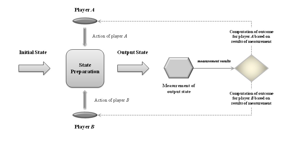
Figure 1: Depiction of the essential elements of a playable classical game.

The essential elements of a playable classical game, as described above, suggest how we may approach the notion of quantizing a game. Strictly speaking we quantize the physical system that is used to implement a classical game. The question of what it means to ‘quantize’ a game is somewhat problematical, as we shall see. With this caveat in mind we now allow the physical elements of our game to be quantum mechanical in nature with the operations of the players being taken from the set of those permitted by quantum mechanics. The measurement of the state becomes a quantum measurement. The results of the measurement become the inputs to the computable function that determines the outcomes for the players. It is important to note that the central ‘philosophy’ of the playable game has not altered by this extension to the quantum domain; just as in the classical case, each player must consider what operations he needs to perform on the initial state in order to produce an output state the measurement of which will yield an optimal result for him, given that the other player is making the same deliberation. Of course the only real difference between games in the classical and quantum domains is that in the latter the physical elements that implement the game are quantum mechanical. The mathematical formalism of game theory applies in both domains.

1.2 Quantum Games

The description of a playable game implemented using classical objects implies a certain underlying physical reality. According to the Copenhagen interpretation, a quantum mechanical description of nature does not assign elements of physical reality until a measurement is made. In classical game theory it is tacitly assumed that that the choice of strategy corresponds to some element of physical reality. In a Turing machine implementation of a classical playable game, once a symbol to describe the strategy choice has been written on the tape it is communicated to the Turing machine, and those bits exist as elements of physical reality on the tape. In quantum mechanics, however, these symbols, now have to be considered as qubits on a quantum mechanical tape, and they do not have any corresponding element of physical reality until they are measured. Furthermore, if we imagine two separate inputs to our quantum Turing machine then not only does quantum mechanics mean that we have to inscribe qubits on our quantum tape, but also that the two quantum tape inputs can be entangled.

Whilst the Turing machine model of a playable game is instructive in highlighting the potential differences between playing games in the classical and quantum domains, it is not the best model for allowing us to draw correspondences between games played in the different domains. The general model of a playable game given in Figure 1 is more suitable. The physical elements of a playable game described in this figure remain unchanged when we consider games in the quantum domain, the only difference being that the input and output states are now quantum states and the actions the players perform to transform the intial state to a desired output state are quantum operations.

In classical playable games, the players have some preference relation over the measurement outcomes and it is these preference relations that determine the choice of operation for the players. In the quantum domain the measurement results are the eigenstates of the measurement operator and the players have some preference relation over these eigenstates. (We only consider von Neumann measurements in this paper. Extending to more generalized quantum measurements adds unnecessary technical detail at present, and essentially introduces no significant new conceptual elements to the game-theoretic description).

In order to be a little more specific we shall consider 2 player games in the quantum domain. The extension to games with more than 2 players is relatively straightforward.

1.2.1 2-Player Quantum Games

We imagine a playable game with players A and B in which some physical system, prepared in an initial quantum state $\left|\psi_{0}\right\rangle$, is fed into a device. The players each perform some unitary transformation on the state to produce an output state $\left|\psi\right\rangle$. This output state is measured, or rather the physical property $\hat{M}$ is measured, the result being one of the eigenstates, $\left|\varphi_{j}\right\rangle$, of the operator $\hat{M}$.

Each player has some preference relation over these eigenstates which we label $P_{A(B)}$. Before enacting their operation on the initial state, each player performs some computation which determines which operation is in their best interests, given that the other player is going to choose an operation which is in his best interests. The preference relations, of course, determine what each player considers to be in their best interests given the constraints. The choice of action is thus some computable function for each player which takes as input the initial state, the possible measurement outcomes, the preference relations and the available operations. Let us make this more explicit.

We let the set of possible states of our quantum system be denoted by $\Psi$. The set of all possible unitary operations on this state will be denoted by $\hat{\Omega}$ where we have used the caret to remind ourselves that this is a set of operators. The ouput state from our device is thus described by some mapping $g:\Psi\times\hat{\Omega}\times\hat{\Omega}\longrightarrow\Psi$. The choice of the element from the set $\hat{\Omega}$ for each player is determined by their knowledge of the initial state, the operations that can be performed on that state, the results of the measurement on the output state and the preference relations over those results. It is important to note that if both players have full knowledge of the parameters of the physical system, including knowledge of each other’s preference relations and available operations, then each player can determine the element of $\hat{\Omega}$ that the other player will pick, assuming rational players, and assuming that the game admits the calculation of such a preferred choice.

We are now in a position to examine some general properties of playable quantum games. These general considerations will be made more concrete when we consider a simple, but highly non-trivial, example of a quantum game in section 3.

2 Playable Quantum Games : General Considerations

It is clear that there is no fundamental difference between playing a game with quantum mechanical objects and state preparation. Indeed, playing a quantum game is state preparation, with the prepared state being determined by the preference relations over the measurement outcomes (along with knowledge of the other important parameters, as discussed above). One important question, from the perspective of game theory, is whether the game parameters lead to the preparation of an equilibrium output state by rational players.

Before we look at the general structure of a quantum game we have proposed it is worth noting here that we are considering here only those quantum games in which the players are allowed to perform some unitary operation on the input state. Measurements are, of course, perfectly allowable quantum operations. A more general treatment of quantum games would allow the players to perform some measurement on the quantum state, possibly followed (or preceded) by some unitary operation. We shall touch upon this briefly when we consider uncertainty in quantum games shortly, but the main details of this more general treatment will be published elsewhere.

The various parameters that characterise a game played using quantum mechanical objects and operations are described below.

$\Psi$ : the set of all possible states of the physical system used to implement the game

$\left|\psi_{0}\right\rangle$ : the initial state of the physical system $(\left|\psi_{0}\right\rangle\in\Psi)\vskip 6.0pt plus 2.0pt minus 2.0pt$

$\Psi_{out}$ : the set of possible output states $(\Psi_{out}\subseteq\Psi)\vskip 6.0pt plus 2.0pt minus 2.0pt$

$\left|\psi\right\rangle$ : the output state, that is, the state produced by the operations of the players on the initial state. $\ (\left|\psi\right\rangle\in\Psi_{out})\vskip 6.0pt plus 2.0pt minus 2.0pt$

$\hat{\Omega}$ : the set of all possible unitary transformations on an element of $\Psi\vskip 6.0pt plus 2.0pt minus 2.0pt$

$\hat{\Omega}_{A(B)}$ : the set of all unitary operations available to player A(B). $\hat{\Omega}_{A(B)}\subseteq\hat{\Omega}$ and $\hat{\Omega}_{A}$ is not necessarily equal to $\hat{\Omega}_{B}$. Note that these sets may contain the indentity operator which simply means that one option that the players can choose is to do nothing to the initial state.

$\hat{\alpha}_{i}$ : an element of the set $\hat{\Omega}_{A}$. $(\hat{\alpha}_{i}\in\hat{\Omega}_{A})\vskip 6.0pt plus 2.0pt minus 2.0pt$

$\hat{\beta}_{j}$ : an element of the set $\hat{\Omega}_{B}$. $(\hat{\beta}_{j}\in\hat{\Omega}_{B})\vskip 6.0pt plus 2.0pt minus 2.0pt$

$\hat{M}$ : the Hermitian operator describing the measurement on the output state $\left|\psi\right\rangle$. The measurement produces the eigenstate $\left|\varphi_{k}\right\rangle$ with probability $\left|\left\langle\varphi_{k}|\psi\right\rangle\right|^{2}\vskip 6.0pt plus 2.0pt minus 2.0pt$

$\left|\varphi_{k}\right\rangle$ : the eigenstates of $\hat{M}$.$\ (\left|\varphi_{k}\right\rangle\in\Psi)\vskip 6.0pt plus 2.0pt minus 2.0pt$

$P_{A(B)}$ : an ordered list of the eigenstates $\left|\varphi_{k}\right\rangle$ such that the 1^st element is A(B)’s most preferred measurement result, the 2^nd element is the 2^nd most preferred result and so on. This is the preference relation for A(B)

The basic sets are depicted in figure 2. If the players do not have access to the full set of operations permitted by quantum mechanics on the initial state then the output state will be a subset of the set of possible states of the quantum system.

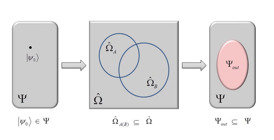
Figure 2: The basic sets of a playable quantum game. An initial state is transformed by the choice of the players’ operation to produce an output state. The players’ choice is determined by their calculation of their expected outcome, given the constraints of the other player’s choice of operation.

Despite the apparent increase in formalism introduced by the quantum description the fundamental questions of game theory remain unaltered. What actions must a player take to ensure that his most advantageous outcome occurs, given that his opponent is making precisely the same deliberation? The determination of what a particular player considers to be advantageous is, of course, encapsulated in the preference relations. Another important game-theoretic question that remains unaltered for a quantum game is whether some equilibrium state is reached as a result of the players’ deliberations.

Some immediate differences do, however, present themselves. The most obvious of these is the difference between classical and quantum measurements. It is not possible, in general, in quantum mechanics to determine the complete configuration of a state. Indeed, it isn’t even correct to ascribe elements of reality to the elements of that configuration. In a classical game the configuration of the output state can, in principle, be measured. In the quantum case we can select a property of the state to measure, but this will not give us complete information about the resultant output state.

This apparent limitation is partly overcome by relating the preference relations of the players to the measurement outcomes. However, the consequence of the quantum description is that some element of stochasticity is introduced by measurement. In other words there will, in general, be a probability distribution over the outcomes in any game played using quantum objects.

2.1 State Preparation

As we have discussed, a game played with quantum mechanical objects is nothing more than state preparation followed by measurement in which the state that is prepared depends upon the players’ consideration of the possible measurement outcomes, the input state and their available operations on that input state. This leads to a certain fluidity in the description of a quantum game similar to that when using the Heisenberg or Schrödinger pictures.

Let us consider a quantum system that is used to play a game in which the input state is $\left|\psi_{0}\right\rangle$, the sets of operations available to the players are given by

$$\hat{\Omega}_{A} =\{\hat{\alpha}_{1},\hat{\alpha}_{2},...,\hat{\alpha}_{p}\}$$

$$\hat{\Omega}_{B} =\{\hat{\beta}_{1},\hat{\beta}_{2},...,\hat{\beta}_{q}\}$$

where we assume, for the moment that $\left[\hat{\alpha}_{k},\hat{\beta}_{j}\right]=0~{}~{}\forall j,k$. The output state is $\left|\psi\right\rangle$, the measurement is characterized by the Hermitian operator $\hat{M}$ which has eigenstates given by $(\left|\varphi\right\rangle_{1},\left|\varphi\right\rangle_{2},...,\left|\varphi\right\rangle_{k})$. Now let us suppose that we change the input state, keeping all other parameters fixed. If the new input state is described by some transformation of the initial state so that $\left|\psi_{0}^{\prime}\right\rangle=T\left|\psi_{0}\right\rangle$ then, in general, a new output state $\left|\psi^{\prime}\right\rangle$ will be produced. If we denote the original game as game 1 and the game with the transformed input as game 2 then the output states in the games are given by

game 1 $$\text{: }\left|\psi\right\rangle=\hat{\beta}_{j}\hat{\alpha}_{k}\left|\psi_{0}\right\rangle$$

game 2 $$\text{: }\left|\psi^{\prime}\right\rangle=\hat{\beta}_{j^{\prime}}\hat{\alpha}_{k^{\prime}}T\left|\psi_{0}\right\rangle$$

where $\mathit{j,j}^{\prime},k$ and$\ k^{\prime}$ describe the operator selections of the players. We can see that game 2 can be thought of as being played with the input state $\left|\psi_{0}\right\rangle$ where player A has a different set of operators to select from given by

$$\hat{\Omega}_{A}^{\prime}=\{\hat{\alpha}_{1}T,\hat{\alpha}_{2}T,...,\hat{\alpha}_{p}T\}$$

We shall call this equivalent game, game 3. Alternatively we could view this as a game played with an input $\left|\psi_{0}\right\rangle$ and the operator sets

$$\hat{\Omega}_{A}^{\prime\prime} =\{T^{-1}\hat{\alpha}_{1}T,T^{-1}\hat{\alpha}_{2}T,...,T^{-1}\hat{\alpha}_{p}T\}$$

$$\hat{\Omega}_{B}^{\prime\prime} =\{T^{-1}\hat{\beta}_{1}T,T^{-1}\hat{\beta}_{2}T,...,T^{-1}\hat{\beta}_{q}T\}$$

in which the state output by the players is then transformed by application of $T$. If we call this new game, game 4, then we can see that games 2, 3 and 4 are all equivalent and they all result in a measurement of $\hat{M}$ on the state $\left|\psi^{\prime}\right\rangle$. We shall call a game for which the output state is written in the form $\left|\psi\right\rangle=\hat{\beta}\hat{\alpha}T\left|\psi_{0}\right\rangle$ an MW-type game. A game for which the output state can be written in the form $\left|\psi\right\rangle=T^{-1}\hat{\beta}\hat{\alpha}T\left|\psi_{0}\right\rangle$ we shall call an EWL-type game. These are the forms of game considered in the previous important work on quantum games [4,8] where $T$ is an entanglement operator producing Bell basis states from the computational basis. Because the calculations the players do are based on the expected outcomes, the MW-type game can be thought of, somewhat informally, as an EWL-type game in which the measurement operator is transformed (and vice versa). In order to make a direct comparison between the two forms of games, however, we should consider the same input state and the same measurement, with the same preference relations over the eigenstates of the measurement operator.

2.1.1 Relation between MW- and EWL-Type Games

An MW-type game produces an output state of the form $\left|\psi\right\rangle_{MW}=\hat{\beta}\hat{\alpha}T\left|\psi_{0}\right\rangle$ and an EWL-type game produces an output state of the form $\left|\psi\right\rangle_{EWL}=T^{-1}\hat{\beta}\hat{\alpha}T\left|\psi_{0}\right\rangle$. If we write $\left|\xi_{0}\right\rangle=T\left|\psi_{0}\right\rangle$ then the MW-type game is nothing more than the general form of quantum game we have introduced. The EWL-type is, in a sense, more ‘artificial’ because a subsequent rotation is imposed upon the output state. If we use a fairly obvious notation for the operator sets so that, for example, $\left(\hat{\Omega}_{A}T\right)=\{\hat{\alpha}_{1}T,\hat{\alpha}_{2}T,...,\hat{\alpha}_{p}T\}$ then the relation between the forms of the MW- and EWL-type games can be seen in the following table for the operator sets of the players where the games in each column are equivalent. We have written the EWL-type game in this table from two perspectives that each ‘eliminate’ the rotation of the final state.

	MW-Type	EWL-Type
Input state : $\left|\xi_{0}\right\rangle\vskip 6.0pt plus 2.0pt minus 2.0pt$	$\hat{\Omega}_{A},\hat{\Omega}_{B}$	$\hat{\Omega}_{A},\left(T^{-1}\hat{\Omega}_{B}\right)$
Input state : $\left|\psi_{0}\right\rangle$	$\ \ \ \left(\hat{\Omega}_{A}T\right),\hat{\Omega}_{B}$	$\ \ \ \ \ \ \ \ \ \ \left(T^{-1}\hat{\Omega}_{A}T\right),\left(T^{-1}\hat{\Omega}_{B}T\right)$

Whether we view the operator sets as fixed or the input states as fixed it is clear that the MW- and EWL-type games will in general lead to different output states. The two EWL-type games in the table are equivalent to an EWL-type game with input state $\left|\xi_{0}\right\rangle$, and operator sets $\hat{\Omega}_{A}$ and $\hat{\Omega}_{B}$ in which a rotation is performed on the resultant state. The rotation clearly alters the distribution of the eigenstates of the measurement operator in the superposition. Of course both players select their operation from their available set in the knowledge that this final rotation will be performed. Alternatively we may view the EWL-type game, as in the table, as one in which no rotation is performed but the players have a transformed set of operators to select from.

As we shall see, it is an interesting question whether rational players would prefer to play a game of the form $\left|\psi\right\rangle=\hat{\beta}\hat{\alpha}\left|\psi_{0}\right\rangle,~{}$ $\left|\psi\right\rangle_{MW}=\hat{\beta}\hat{\alpha}T\left|\psi_{0}\right\rangle,$ or $\left|\psi\right\rangle_{EWL}=T^{-1}\hat{\beta}\hat{\alpha}T\left|\psi_{0}\right\rangle$ for a given $T$.

2.2 Non-Commuting Games

The next important element that a quantum mechanical description introduces is the notion that operations on the input state do not necessarily commute. Thus, in general, it matters whether player A or player B performs their operation first. If, as above, we let the set of operations available to player A(B) be denoted by $\hat{\Omega}_{A(B)}$ where $\hat{\Omega}_{A(B)}\subseteq\hat{\Omega}$ and $\hat{\Omega}_{A}$ is not necessarily equal to $\hat{\Omega}_{B}$ then a quantum game is non-commuting if there is at least one element $\hat{\alpha}_{i}\in\hat{\Omega}_{A}$ such that $\left[\hat{\alpha}_{i},\hat{\beta}_{j}\right]\neq 0$ for at least one $j$ where $\hat{\beta}_{j}\in\hat{\Omega}_{B}$.

Let us suppose that the players have access to a discrete set of operations such that the cardinality of $\hat{\Omega}_{A}$ is p and the cardinality of $\hat{\Omega}_{B}$ is q. If player A makes the first move then the possible output states are described by a $p\times q$ matrix with elements given by $\left|\psi_{ij}^{BA}\right\rangle=\hat{\beta}_{j}\hat{\alpha}_{i}\left|\psi_{0}\right\rangle$. If player B makes the first move then the possible output states are described by a $q\times p$ matrix with elements given by $\left|\psi_{ij}^{AB}\right\rangle=\hat{\alpha}_{j}\hat{\beta}_{i}\left|\psi_{0}\right\rangle$. Thus if $\hat{\Omega}_{A}\neq\hat{\Omega}_{B}$ we have that, in general, $\Psi_{out}^{BA}\neq\Psi_{out}^{AB}$.

Thus, in a non-commuting game a player’s choice of operation may be determined by whether he operates on the input state before or after the other player. Of course, depending on the elements of the sets $\hat{\Omega}_{A(B)}$, it is possible that a different equilibrium state is reached in the two situations. Indeed, the choice of operation for each rational player will in general be different depending on which player makes the first move. This immediately raises the intriguing question of what happens if the players don’t know which of their operations is performed by the physical device first.

2.2.1 Commutativity in Equivalent MW-Type Games

As we have seen, there are different equivalent perspectives for an MW-type game. We shall label these as MW_i so that we have

• MW₀ : input state $\left|\xi_{0}\right\rangle=T\left|\psi_{0}\right\rangle$, operator sets $\hat{\Omega}_{A},\hat{\Omega}_{B}$, no final state rotation

• MW₁ : input state $\left|\psi_{0}\right\rangle$, operator sets $\left(\hat{\Omega}_{A}T\right),\hat{\Omega}_{B}$, no final state rotation

• MW₂ : input state $\left|\psi_{0}\right\rangle$, operator sets $\left(T^{-1}\hat{\Omega}_{A}T\right),\left(T^{-1}\hat{\Omega}_{B}T\right)$, final state rotation by $T$

Each of these perspectives leads to the production of the same output state and therefore the expected outcomes for the players are unchanged in each of these perspectives. We shall suppose that MW₀ is a commuting game so that $\left[\hat{\alpha}_{k},\hat{\beta}_{j}\right]=0~{}~{}\forall j,k$.

Clearly MW₁ is a non-commuting game, in general, and it is only equivalent if player A plays first. The MW-type game with input $\left|\psi_{0}\right\rangle$, operator sets $\hat{\Omega}_{A},\left(\hat{\Omega}_{B}T\right)$ in which player B plays first, is also equivalent to MW₀ when MW₀ is a commuting game. Accordingly we denote these equivalent games as MW_1A and MW_1B where the additional subscript denotes which player plays first.

If we denote the elements of the operator sets in MW₂ as $\hat{\alpha}_{k}^{\prime}$ and $\hat{\beta}_{j}^{\prime}$ then the commutation relation between them is given by

$$\left[\hat{\alpha}_{k}^{\prime},\hat{\beta}_{j}^{\prime}\right]=T^{-1}\left[\hat{\alpha}_{k},\hat{\beta}_{j}\right]T$$

so that if MW₀ is a commuting game MW₂ is also a commuting game.

2.2.2 Commutativity in Equivalent EWL-Type Games

The different equivalent perspectives in EWL-type games are given by

• EWL_0A : input state $\left|\xi_{0}\right\rangle=T\left|\psi_{0}\right\rangle$, operator sets $\hat{\Omega}_{A},\left(T^{-1}\hat{\Omega}_{B}\right)$, no final state rotation, player A plays first

• EWL_0B : input state $\left|\xi_{0}\right\rangle=T\left|\psi_{0}\right\rangle$, operator sets $\left(T^{-1}\hat{\Omega}_{A}\right),\hat{\Omega}_{B}$, no final state rotation, player B plays first

• EWL₁ : input state $\left|\psi_{0}\right\rangle$, operator sets $\left(T^{-1}\hat{\Omega}_{A}T\right),\left(T^{-1}\hat{\Omega}_{B}T\right)$, no final state rotation, commuting game if $\left[\hat{\alpha}_{k},\hat{\beta}_{j}\right]=0~{}~{}\forall j,k$.

• EWL_2A : input state $\left|\psi_{0}\right\rangle$, operator sets $\left(\hat{\Omega}_{A}T\right),\left(T^{-1}\hat{\Omega}_{B}\right)$, no final state rotation, player A plays first

• EWL_2B : input state $\left|\psi_{0}\right\rangle$, operator sets $\left(T^{-1}\hat{\Omega}_{A}\right),\left(\hat{\Omega}_{B}T\right)$, no final state rotation, player B plays first

• EWL_3A : input state $\left|\psi_{0}\right\rangle$, operator sets $\left(\hat{\Omega}_{A}T\right),\hat{\Omega}_{B}$, final state rotation by $T^{-1}$, player A plays first

• EWL_3B : input state $\left|\psi_{0}\right\rangle$, operator sets $\hat{\Omega}_{A},\left(\hat{\Omega}_{B}T\right)$, final state rotation by $T^{-1}$, player B plays first

All these are different but equivalent perspectives leading to the production of the same state upon which a measurement of $\hat{M}$ is performed, provided that we have $\left[\hat{\alpha}_{k},\hat{\beta}_{j}\right]=0~{}~{}\forall j,k$. As an example of the drastic difference that the order of play can make for a non-commuting game consider the perspectives EWL_2A and EWL_2B. If we now swap the order of play in each of these perspectives we obtain the commuting game with input $\left|\psi_{0}\right\rangle$ and operator sets $\hat{\Omega}_{A}$ and $\hat{\Omega}_{B}$.

2.3 Equilibrium in Quantum Games

In game theory an equilibrium state is reached when the two players select a strategy they would not change irrespective of the other player’s choice. Such a state is a Nash equilibrium. We can see from the general model of a playable game that if such an equilibrium exists then it leads to a particular output state. In quantum games, therefore, the existence of an equilibrium implies that a particular output state is also produced (or possibly one of a family of physically equivalent output states that yield the same distribution over the measurement outcomes).

If we label the eigenstates of the measurement operator as $\left|\varphi_{k}\right\rangle$ then the output state can be expanded in terms of these eigenstates

$$\left|\psi\right\rangle={\displaystyle\sum\limits_{k=1}^{n}}\left|\varphi_{k}\right\rangle\left\langle\varphi_{k}|\psi\right\rangle$$

and the result of the measurement is the eigenstate $\left|\varphi_{j}\right\rangle$ with probability $\left|\left\langle\varphi_{j}|\psi\right\rangle\right|^{2}$. Intuitively, we might suppose that each player will choose an operation that maximises the probability of their most desired eigenstate according to their preference relations, given that the other player is choosing his operation to achieve the same end according to his preference relations. Thus we can imagine that there are two competing ‘forces’ trying to rotate the initial state to some preferred direction. This geometric approach, briefly outlined below, has been explored elsewhere [21,22].

In general the measurement of the output state will lead to a distribution of outcomes and consequently the players must seek to optimise their expected outcomes. Let us suppose that player A performs his operation first. Player A will choose an $\hat{\alpha}_{i}$ so that his expected outcome is optimised whatever B subsequently does. Likewise, B will choose a $\hat{\beta}_{j}$ so that his expected outcome is optimised whatever A has chosen.

Let us consider a measurement $\hat{M}$ with n eigenstates given by the list $(\left|\varphi_{1}\right\rangle,\left|\varphi_{2}\right\rangle,...,\left|\varphi_{n}\right\rangle)$ which for convenience we can write as the list of numbers $\varphi=(1,2,..,n)$. The preference relation of player A is simply a permutation of this list such that the first state in the list is his most preferred, the second state his second most preferred, and so on, and similarly for player B. If we let $\pi^{A(B)}(k)$ be functions that take the integers from 1 to n as input and output the number from $\varphi$ that represents the k^th most preferred state of player A(B) then we can write the preference relations for the players as an ordered n-tuple of the integers from 1 to n.

$$P_{A} =(\pi^{A}(1),\pi^{A}(2),...,\pi^{A}(n))$$

$$P_{B} =(\pi^{B}(1),\pi^{B}(2),...,\pi^{B}(n))$$

In order to calculate an expected outcome we must assign some numerical value, or weight, to each of the eigenstates that encapsulates the notion of preference. In crude terms this numerical value can be thought of as the payoff for each state. For simplicity we attach the numerical weight n to the most preferred state, and the weight 1 to the least preferred state, for each player. Thus if the measurement result yields A’s most preferred state then player A would receive n cupcakes, for example. The expected payoffs for the players, denoted by $E_{ij}^{A(B)}$, if the operations $\hat{\alpha}_{i}$ and $\hat{\beta}_{j}$ are chosen, are then given by

$$E_{ij}^{A} =\sum_{k=1}^{n}(n-k+1)\left|\left\langle\varphi_{\pi^{A}(k)}|\hat{\beta}_{j}\hat{\alpha}_{i}|\psi_{0}\right\rangle\right|^{2}$$

$$E_{ij}^{B} =\sum_{k=1}^{n}(n-k+1)\left|\left\langle\varphi_{\pi^{B}(k)}|\hat{\beta}_{j}\hat{\alpha}_{i}|\psi_{0}\right\rangle\right|^{2}$$

These quantities define a matrix of expected outcomes for each player, the elements denoting each choice of operation $(\hat{\alpha}_{i},\hat{\beta}_{j})$. We have assumed that player A plays first and the knowledge of the order of the moves can make a difference to the strategy selection. In a non-commuting game the order of play must be specified. For a commuting game in which there is no specification of the order of play then if A and B can find operators $(\hat{\alpha}_{i},\hat{\beta}_{j})$ such that

$$\sum_{j}E_{ij}^{A} >\sum_{j}E_{pj}^{A}~{}~{}~{}~{}(\forall p\neq i)$$

$$\sum_{i}E_{ij}^{B} >\sum_{i}E_{iq}^{B}~{}~{}~{}~{}(\forall q\neq j)$$

then an equilibrium output state is obtained given by $\left|\psi\right\rangle=\hat{\beta}_{j}\hat{\alpha}_{i}\left|\psi_{0}\right\rangle=\hat{\alpha}_{i}\hat{\beta}_{j}\left|\psi_{0}\right\rangle$. The players thus each maximise their expected outcomes over the choices of the other player.

For a non-commuting game in which player A plays first, the strategy selection is influenced by the order of play. Player A must select his strategy knowing that B has the advantage of playing second. Player A examines the matrix of expected outcomes for player B and looks at the choices of B that maximise B’s expected outcome for every choice of player A’s operator. This gives A a list of operator pairs. From these A now selects the one that maximises his expected outcome.

2.3.1 The geometric approach to equilibrium

When playing a game with quantum objects the players have some preference over the measurement outcomes which are the eigenstates of the measurement operator. We have written these above simply as an ordered list of the labels for the eigenstates. More explicitly we can write these preferences as

Player A $$\text{:}|\varphi_{\pi^{A}(1)}>~{}\succ~{}|\varphi_{\pi^{A}(2)}>~{}\succ...\succ~{}|\varphi_{\pi^{A}(n)}>$$

Player B $$\text{:}|\varphi_{\pi^{B}(1)}>~{}\succ~{}|\varphi_{\pi^{B}(2)}>~{}\succ...\succ~{}|\varphi_{\pi^{B}(n)}>$$

Any output state from the game, before measurement, can be described by

$$\left|\psi\right\rangle=\sum_{k=1}^{n}\left|\varphi_{\pi^{A}(k)}\right\rangle\left\langle\varphi_{\pi^{A}(k)}|\psi\right\rangle=\sum_{k=1}^{n}\left|\varphi_{\pi^{B}(k)}\right\rangle\left\langle\varphi_{\pi^{B}(k)}|\psi\right\rangle$$

Let us consider the subsets $\Psi_{\pi^{A(B)}}$ of $\Psi$ given by the states

$$\left|\psi(\pi^{A(B)})\right\rangle=\left\langle\varphi_{\pi^{A(B)}(1)}|\psi\right\rangle\left|\varphi_{\pi^{A(B)}(1)}\right\rangle+\left\langle\varphi_{\pi^{A(B)}(2)}|\psi\right\rangle\left|\varphi_{\pi^{A(B)}(2)}\right\rangle+...+\left\langle\varphi_{\pi^{A(B)}(n)}|\psi\right\rangle\left|\varphi_{\pi^{A(B)}(n)}\right\rangle$$

where the probability amplitudes respect the preferences so that

$$\left|<\varphi_{\pi^{A(B)}(1)}|\psi>\right|^{2}~{}>~{}\left|<\varphi_{\pi^{A(B)}(2)}|\psi>\right|^{2}~{}>...>~{}\left|<\varphi_{\pi^{A(B)}(n)}|\psi>\right|^{2}$$

The subsets $\Psi_{\pi^{A(B)}}$ define regions of the full Hilbert space of the outputs. These subsets are not subspaces and the elements of $\Psi_{\pi^{A}}$ are not, in general, orthogonal to those of $\Psi_{\pi^{B}}$. Each player would act in such a way as to try to direct the output state into their respective regions of Hilbert space. The final output state will, therefore, be some state that would be ‘as equidistant’ from their respective regions that the players can achieve with their given operator sets. The resultant state, if this can be achieved, will be the Nash equilibrium position for the quantum game. Some ramifactions of this approach are discussed in [21,22].

2.4 The Preference Relations

Let us suppose, as above, that the players have access to a discrete set of operations such that the cardinality of $\hat{\Omega}_{A}$ is p and the cardinality of $\hat{\Omega}_{B}$ is q. If player A makes the first move then the possible output states are described by an $p\times q$ matrix with elements given by $\left|\psi_{ij}^{BA}\right\rangle=\hat{\beta}_{j}\hat{\alpha}_{i}\left|\psi_{0}\right\rangle$. The players each have a preference relation over the eigenstates $\left|\varphi_{k}\right\rangle$ of the measurement operator $\hat{M}$. If n is the cardinality of the set of eigenstates then, in general, $n\neq pq$. There will often be a greater number of possible output states that can be produced by the players than the number of possible measurement outcomes. Indeed, as we shall see, the possible ouput states can form a continuum whereas the measurement outcomes consist of a small discrete set of possibilities.

As we have discussed in the previous section, each player can determine a matrix of expected outcomes where the elements $E_{ij}^{A(B)}$ give the expected outcome for player $A(B)$ for the possible output state $\left|\psi_{ij}\right\rangle=\hat{\beta}_{j}\hat{\alpha}_{i}\left|\psi_{0}\right\rangle$. Clearly, this leads to an ordered list of expected outcomes in which each player ranks each possible output state according to its expected outcome for him. Thus the preference relation over the eigenstates of the measurement operator for player $A(B)$ induces a preference relation over the possible output states.

Let us suppose that the measurement operator for some 2-player quantum game is rotated by the action of an operator $T$ such that the new meaurement operator is $\hat{M}^{\prime}=T^{-1}\hat{M}T$. The eigenstates of $\hat{M}^{\prime}$ are $\left|\varphi_{k}^{\prime}\right\rangle=T\left|\varphi_{k}\right\rangle$. If the players maintain the same preference relation over the new eigenstates so that $\left(\pi^{A}(k)\right)^{\prime}=\pi^{A}(k)$ and $\left(\pi^{B}(k)\right)^{\prime}=\pi^{B}(k)$ then, in order for the players to be playing the same game with respect to the new measurement basis the various components have to be transformed according to

$$\left|\psi_{0}^{\prime}\right\rangle =T\left|\psi_{0}\right\rangle$$

$$\hat{\alpha}_{i}^{\prime} =T\hat{\alpha}_{i}T^{-1}$$

$$\hat{\beta}_{j}^{\prime} =T\hat{\beta}_{j}T^{-1}$$

With these transformations the expected outcomes for player A with respect to the new measurement basis are given by

$$\left(E_{ij}^{A}\right)^{\prime}=\sum_{k=1}^{n}(n-k+1)\left|\left\langle\varphi_{\pi^{A}(k)}^{\prime}|\hat{\beta}_{j}^{\prime}\hat{\alpha}_{i}^{\prime}|\psi_{0}^{\prime}\right\rangle\right|^{2}=\sum_{k=1}^{n}(n-k+1)\left|\left\langle\varphi_{\pi^{A}(k)}|\hat{\beta}_{j}\hat{\alpha}_{i}|\psi_{0}\right\rangle\right|^{2}=E_{ij}^{A}$$

and similarly for player B. Thus the expected outcomes remain unaltered, provided that both the initial state and the operator choices of the players are transformed.

2.5 Invertible Games

We define an invertible game as one in which one, or both, players can invert the operations performed by the other player. For example, let us suppose that the set of operations available to A is given by $\{\hat{\alpha}_{1},\hat{\alpha}_{2},...,\hat{\alpha}_{p}\}$ then the game is invertible if B has a set of available operations that includes the inverses of these elements, that is, the set of operations available to B is given by $\{\hat{\beta}_{1},\hat{\beta}_{2},...,\hat{\beta}_{q},\hat{\alpha}_{1}^{-1},\hat{\alpha}_{2}^{-1},...,\hat{\alpha}_{p}^{-1}\}$. There is nothing intrinsically quantum mechanical about such games for we could construct a playable classical game in which the operations of one, or both, players could be inverted by the other.

It is clear that an equilibrium state, in the sense that an equilibrium state is the optimal choice for both players, does not exist for an invertible game. In order to see this we shall consider a game in which A moves first. If we assume rational players then A’s preferred choice of move given the constraints, if it exists, is computable by both A and B. Therefore B simply needs to follow A’s move with $\hat{\beta}_{k}\hat{\alpha}^{-1}$ where $\hat{\beta}_{k}$ operating on $\left|\psi_{0}\right\rangle$ maximises B’s expected outcome. Of course, this implies that there is no such rational choice for A. In fact, A’s best strategy in this situation is to select his move with some distribution.

One immediate consequence of this is that if we allow players to access every possible operation on the input state allowed by quantum mechanics then there cannot be an equilibrium output state. In order to reach some kind of equilibrium we must restrict the available strategies in some way. This, of course, restricts the possible output states. This consideration becomes crucial when we consider our simple, but important, example of a quantum game.

If we suppose that $\hat{\Omega}_{A}=\hat{\Omega}_{B}$ and that the elements of these sets form a group then the resulting game will be invertible. For games which satisfy this condition there can be no equilibrium state.

2.6 Factorable Quantum Games

We define a factorable game as one in which there is no element of entanglement. In other words, the input states are tensor product states and the available operations only lead to output states that are also tensor product states. Factorable games can still be non-commuting and invertible.

2.7 Sequential Quantum Games

A sequential game is one in which the players make a sequence of moves. So, for example, player A goes first, followed by player B. Player A then makes his second move, followed by player B, and so on. If we let $\hat{\alpha}(i)$ be the i^th operation of player B and $\hat{\beta}(i)$ be the i^th operation of player B then the output state after m moves is given by

$$\left|\psi\right\rangle=\hat{\beta}(m)\hat{\alpha}(m)...\hat{\beta}(2)\hat{\alpha}(2)\hat{\beta}(1)\hat{\alpha}(1)\left|\psi_{0}\right\rangle$$

After each move we can think of the resultant state as being equivalent to some new input state, thus a sequential game is a sequence of single-move games in which the output state from the previous game becomes the input state to the next. If we let $\left|\psi_{0}^{k}\right\rangle$ be the state after the k^th move of the players then any sequential game of m moves can be thought of as a single-move game in which the input state is given by $\left|\psi_{0}^{m-1}\right\rangle$ with

$$\left|\psi_{0}^{m-1}\right\rangle=\hat{\beta}(m-1)\hat{\alpha}(m-1)...\hat{\beta}(2)\hat{\alpha}(2)\hat{\beta}(1)\hat{\alpha}(1)\left|\psi_{0}\right\rangle$$

Alternatively we can factor the sequence of operations into two new operators $\hat{\alpha}^{\prime}$ and $\hat{\beta}^{\prime}$ where, for example,

$$\hat{\alpha}^{\prime} =\hat{\beta}(k)\hat{\alpha}(k)...\hat{\beta}(2)\hat{\alpha}(2)\hat{\beta}(1)\hat{\alpha}(1)$$

$$\hat{\beta}^{\prime} =\hat{\beta}(m)\hat{\alpha}(m)...\hat{\beta}(k+2)\hat{\alpha}(k+2)\hat{\beta}(k+1)\hat{\alpha}(k+1)$$

Thus the sequential game of m moves is equivalent to a single-move game in which the operators $\hat{\alpha}^{\prime}$ and $\hat{\beta}^{\prime}$ are included in A and B’s set of available operators, respectively. Note that there is no unique way to perform this factorization.

These considerations also show us that any single-move game can be represented by some equivalent sequential game of m moves. Of course there is no unique m-move representation. In fact there are an infinite number of m-move representations of any single-move game. By equivalent we mean that the same output states are produced and the players receive the same expected outcomes. In game theory terms the players are in effect playing a different game. Constructing the equivalent representations of a single-move game or an m-move game is not, in general, a trivial exercise.

If a single-move game has an equilibrium then all equivalent sequential m-move games also reach an equilibrium. Alternatively if we construct an equivalent sequential m-move game that reaches equilibrium then the single-move game also reaches equilibrium. Indeed, if it can be shown that one member of the class of equivalent m-move games reaches equilibrium then all games in the class also reach equilibrium, as does the equivalent single-move game.

2.8 Equilibrium as a Limit of a Sequential Game

Another way to think of the production of an equilibrium state is as the limit of a sequential game. Let us suppose that two players play a sequential game with a no limit on the number of moves they can make. If they both reach a point such that they do not wish to make another move after a finite number of moves then the resultant output state is an equilibrium state. Conversely, if no such limit exists then there cannot be an equilibrium.

If we consider an invertible sequential game with no fixed number of moves then we can see that the players would never reach a point where they would wish to stop. If we extend a single-move game to a sequential game with no fixed number of moves then the resultant game may not have an equilibrium state even if the single-move game reaches equilibrium. This is because the subsequent moves potentially give the players access to a larger set of operations than those for the single-move game. In order to see this let us consider a sequential game with just 2 moves allowed. The output state is given by

$$\left|\psi\right\rangle=\hat{\beta}(2)\hat{\alpha}(2)\hat{\beta}(1)\hat{\alpha}(1)\left|\psi_{0}\right\rangle$$

Thus, in effect, A chooses the operator $\hat{\alpha}^{\prime}=\hat{\alpha}(2)\hat{\beta}(1)\hat{\alpha}(1)$ which may not be included in his set of available operations for his first move. We could also view this as a single-move game in which A plays $\hat{\alpha}(1)$ and B plays $\hat{\beta}^{\prime}=\hat{\beta}(2)\hat{\alpha}(2)\hat{\beta}(1)$ Thus if the original single-move game has initial state $\left|\psi_{0}\right\rangle$ and sets $\hat{\Omega}_{A}=\{\hat{\alpha}_{1},\hat{\alpha}_{2},...,\hat{\alpha}_{p}\}$ and $\hat{\Omega}_{B}=\{\hat{\beta}_{1},\hat{\beta}_{2},...,\hat{\beta}_{q}\}$ then the sequential game with 2 moves is equivalent to the single-move game with initial state $\left|\psi_{0}\right\rangle$ and sets $\hat{\Omega}_{A}^{\prime}=\{\hat{\alpha}_{1},\hat{\alpha}_{2},...,\hat{\alpha}_{p},\hat{\alpha}^{\prime}\}$ and $\hat{\Omega}_{B}=\{\hat{\beta}_{1},\hat{\beta}_{2},...,\hat{\beta}_{q}\}$. It is also equivalent to the single-move game with initial state $\left|\psi_{0}\right\rangle$ and sets $\hat{\Omega}_{A}=\{\hat{\alpha}_{1},\hat{\alpha}_{2},...,\hat{\alpha}_{p}\}$ and $\hat{\Omega}_{B}^{\prime}=\{\hat{\beta}_{1},\hat{\beta}_{2},...,\hat{\beta}_{q},\hat{\beta}^{\prime}\}$.

The 2-move sequential game also gives us a way of characterizing equilibrium for a single-move game. If the players in a 2-move game would choose the identity operation from their set of available operators for their second move, this implies that their first move was the best they could make and they cannot improve upon it by playing another. Thus equilibrium is reached for the single-move game if the second move of a 2-move sequential game is the identity operation, for both players. Equilibrium for an m-move game can also be defined in a similar fashion; if the $(m+1)^{th}$ move is the identity element for both players, then the game has reached equilibrium.

2.9 Quantum Games and Uncertainty

We have seen one way in which considerations of non-commutativity impact upon quantum games. Let us now look at another way in which this can arise within the context of a quantum game. Consider the situation shown in figure 3 where we have 2 quantum games. In both games the same input state $\left|\psi_{0}\right\rangle$ is used and the players have access to the same operations $\hat{\Omega}_{A}=\{\hat{\alpha}_{1},\hat{\alpha}_{2},...,\hat{\alpha}_{p}\}$ and $\hat{\Omega}_{B}=\{\hat{\beta}_{1},\hat{\beta}_{2},...,\hat{\beta}_{q}\}$. The games differ, therefore, only in the measurement of the output state. In game 1 the measurement performed is $\hat{M}$ and in game 2 the measurement is $\hat{N}$.

Adopting a slightly different notation to that used previously, the eigenvalues and eigenstates of these operators are given by

$$\hat{M}\left|\mu_{k}\right\rangle =\mu_{k}\left|\mu_{k}\right\rangle$$

$$\hat{N}\left|\nu_{k}\right\rangle =\nu_{k}\left|\nu_{k}\right\rangle$$

and we assume that $\left[\hat{M},\hat{N}\right]\neq 0$. The set of possible output states in both games is the same. The preference relations in game 1 are given by

$$P_{A}^{1} =\left(\left|\mu_{\pi^{A}(1)}\right\rangle,\left|\mu_{\pi^{A}(2)}\right\rangle,...,\left|\mu_{\pi^{A}(n)}\right\rangle\right)\equiv(\pi^{A}(1),\pi^{A}(2),...,\pi^{A}(n))$$

$$P_{B}^{1} =\left(\left|\mu_{\pi^{B}(1)}\right\rangle,\left|\mu_{\pi^{B}(2)}\right\rangle,...,\left|\mu_{\pi^{B}(n)}\right\rangle\right)\equiv(\pi^{B}(1),\pi^{B}(2),...,\pi^{B}(n))$$

Let us consider the unitary transformation $T$ which takes the state $\left|\mu_{k}\right\rangle$ into the state $\left|\nu_{k}\right\rangle$. This can be written in the form

$$T=\sum_{j=1}^{n}\left|\nu_{j}\right\rangle\left\langle\mu_{j}\right|$$

and we suppose that the preference relations for game 2 are given by this transformation applied to the preferences of game 1 so that

$$P_{A}^{2} =\left(T\left|\mu_{\pi^{A}(1)}\right\rangle,T\left|\mu_{\pi^{A}(2)}\right\rangle,...,T\left|\mu_{\pi^{A}(n)}\right\rangle\right)\equiv(\pi^{A}(1),\pi^{A}(2),...,\pi^{A}(n))$$

$$P_{B}^{2} =\left(T\left|\mu_{\pi^{B}(1)}\right\rangle,T\left|\mu_{\pi^{B}(2)}\right\rangle,...,T\left|\mu_{\pi^{B}(n)}\right\rangle\right)\equiv(\pi^{B}(1),\pi^{B}(2),...,\pi^{B}(n))$$

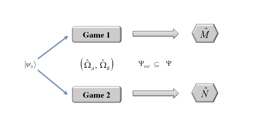
Figure 3: Two quantum games characterized by the same input state and operations but different measurements on the output state.

It is clear that the players need to choose different strategies for each game, in general. This can be most clearly seen if we assume that $\hat{M}$ and $\hat{N}$ are maximally conjugate. Let us further assume that the operator sets for the players are such that they produce eigenstates of $\hat{M}$ in game 1. In game 2, these same operations lead to states that have equal probability amplitudes, up to a phase factor, in the eigenstates of $\hat{N}$. Thus in game 2 with these sets of operators there is no preferred strategy since all strategies lead to the same expected outcome (this outcome is $(n+1)/2$ if we adopt the weighting convention for the outcomes of the previous sections).

It is an interesting question as to whether the uncertainty principle itself can be cast in the form of a game. In this viewpoint we would treat the different measurements as competing in some sense. Of course we would have to consider the more general form of a quantum game in which the players were allowed to perform a measurement. As we have seen in the above example, localizing the output state to a particular eigenstate in game 1 produces a corresponding uncertainty in the measurement of game 2 for that output state. This will lead to a corresponding spread in the outcomes for game 2 when the output state is localized on an eigenstate of game 1. Intuitively we would expect that as we reduced the variance in the outcomes for game 1 we would increase those of game 2 and vice versa.

Let us suppose that the output state for game 1 is the state $\left|\psi\right\rangle$ the expected outcomes for player A in games 1 and 2 with this output state are

$$E_{1}^{A}\left(\left|\psi\right\rangle\right) =\sum_{k=1}^{p}\varpi_{\pi^{A}(k)}\left|\left\langle\mu_{k}|\psi\right\rangle\right|^{2}$$

$$E_{2}^{A}\left(\left|\psi\right\rangle\right) =\sum_{k=1}^{p}\varpi_{\pi^{A}(k)}\left|\left\langle\nu_{k}|\psi\right\rangle\right|^{2}$$

and we have labelled the numerical weights attached to the outcomes as $\varpi_{j}$ with $\varpi_{1}>\varpi_{2}>...>\varpi_{p}$. If we define the Hermitian operators $\hat{E}_{1}$ and $\hat{E}_{2}$ by

$$\hat{E}_{1} =f\left(\hat{M}\right)=\sum_{j=1}^{p}\varpi_{\pi^{A}(j)}\left|\mu_{j}\right\rangle\left\langle\mu_{j}\right|$$

$$\hat{E}_{2} =f\left(\hat{N}\right)=\sum_{j=1}^{p}\varpi_{\pi^{A}(j)}\left|\nu_{j}\right\rangle\left\langle\nu_{j}\right|$$

then the product of the variances of the outcomes in the two games satisfies the uncertainty relation

$$\left(\Delta\hat{E}_{1}\right)^{2}\left(\Delta\hat{E}_{2}\right)^{2}\geq\frac{1}{4}\left|\left\langle\psi\right|\left[f\left(\hat{M}\right),f\left(\hat{N}\right)\right]\left|\psi\right\rangle\right|^{2}$$

Of course the function $f$ is defined by a look-up table being a function that has eigenvalues that are the weights arranged according to the preference relations.

2.10 Quantum Dynamics as a Game

The solution to the time-independent Schrödinger equation can be expressed by

$$\left|\psi(t)\right\rangle=e^{-i\hat{H}t}\left|\psi(0)\right\rangle$$

where we have set $\hbar=1$. The time-evolution operator $\hat{T}=e^{-i\hat{H}t}$ is unitary. It is clear that this operator can be factored into the product of two unitary operators $\hat{\alpha}$ and $\hat{\beta}$ so that $\hat{T}=\hat{\beta}\hat{\alpha}$. There is obviously no unique way to perform this factorisation. The evolution of the initial state $\left|\psi(0)\right\rangle$ is fixed by the Hamiltonian and yields the output state $\left|\psi(t)\right\rangle$. This output state can be thought of as the equilibrium state of some quantum game in which $\hat{\alpha}$ and $\hat{\beta}$ represent the optimum strategy choices for the two players. Thus we can think of the time evolution of a quantum system as being the result of some game between two players. Constructing such a game and the associated preference relations and sets $\hat{\Omega}_{A}$ and $\hat{\Omega}_{B}$ is not, however, a trivial task. There are, in general, an infinite number of such games for any quantum evolution that takes $\left|\psi(0)\right\rangle$ to $\left|\psi(t)\right\rangle$.

It is clear from our previous discussion that if either of the players has access to the full set of quantum mechanically allowed operations on a given physical system used in a playable game then an equilibrium state cannot be reached. If we are to associate a playable game with the evolution of some state, then the operations available to the players are restricted by the form of the Hamiltonian. In other words the Hamiltonian restricts the set of output states. Note that whilst we can always associate some game with the time evolution of a physical system, it may not always be possible to construct a physically meaningful Hamiltonian that will yield the equilibrium state of a given two-player game. However, if we can do this, then the solution of the time-independent Schrödinger equation yields the equilibrium state for that game.

3 2-Player 2-Qubit Games

In what follows we shall consider a simple quantum system which can be used to play a variety of playable quantum games. In this system we imagine that two spin-1/2 particles are prepared in some state and input into some device which allows the players to each perform a unitary operation on these particles (or a sequence of such operations). The spin-1/2 particles are then transmitted to some measurement device. The result of this measurement determines the outcomes for the players.

We shall label the particles with A and B although this is not to be understood that particle A is only operated upon by player A necessarily, and similarly for particle B. In the spin-z basis where the spin-up and spin-down states are labelled with 1 and 0, respectively, the general state of the two particles can be written as

$$\left|\psi\right\rangle=\alpha\left|0,0\right\rangle+\beta\left|0,1\right\rangle+\gamma\left|1,0\right\rangle+\delta\left|1,1\right\rangle$$

where we have written, for example, $\left|0,0\right\rangle=\left|0\right\rangle_{z,A}\otimes\left|0\right\rangle_{z,B}$. We shall drop the labels z, A and B for convenience, except where ambiguity might arise. The particular quantum game that is played with this physical system is determined by the input state of the two spin-1/2 particles, $\left|\psi_{0}\right\rangle$, the set of operations $\hat{\Omega}_{A(B)}$ available to player A(B), the Hermitian operator characterizing the measurement, $\hat{M}$, and the preference relations of player A(B), $P_{A(B)}$, over the eigenstates of the measurement operator $\hat{M}$.

3.1 Playing a Classical Game with Quantum Coins

Let us suppose that the initial state of our particles is given by $\left|\psi_{0}\right\rangle=\left|0,0\right\rangle$ and that the measurement is simply the independent determination of the spin in the z-direction of both particles so that  $\hat{M}=\hat{\sigma}_{z}^{A}\otimes\hat{\sigma}_{z}^{B}$. The possible results of the measurement are thus given by the eigenstates of $\hat{M}$ which are given by

$$\left|\varphi_{1}\right\rangle =\left|0,0\right\rangle$$

$$\left|\varphi_{2}\right\rangle =\left|0,1\right\rangle$$

$$\left|\varphi_{3}\right\rangle =\left|1,0\right\rangle$$

$$\left|\varphi_{4}\right\rangle =\left|1,1\right\rangle$$

Each player will have some (different) preference relation over these states. We now suppose that the device that implements the game will only allow the players to flip the spin of one particle and we further suppose that player A(B) is restricted to operations only on particle A(B). One possible representation of the sets of operations available to the players is therefore given by

$$\hat{\Omega}_{A} =\{\hat{I},\exp\left(i\frac{\pi}{2}\hat{\sigma}_{x}^{A}\right)\}$$

$$\hat{\Omega}_{B} =\{\hat{I},\exp\left(i\frac{\pi}{2}\hat{\sigma}_{x}^{B}\right)\}$$

where $\hat{I}$ is the identity operator and $\hat{\sigma}_{x}^{A(B)}$ is the spin operator in the x-direction for particle A(B).

The preference relations for the players can be written as an ordered list of the numbers 1,2,3, and 4 in an obvious shorthand notation. For example, the preference relations

$$P_{A} =(2,1,4,3)$$

$$P_{B} =(3,1,4,2)$$

are those for the iconic game of Prisoner’s Dilemma. The preference relations alone do not completely specify a game, however, and the strategy set for the players must also be taken into account. In classical games where there are two choices in the strategy sets $S^{A(B)}$ so that there are 4 possible outcomes, there are 432 possible pairs of preference relations in which the first members of the lists differs. The quantum system we have described, with the strategy set limited to a spin flip or identity operation, can implement all 432 of these classical games as there is a direct one-to-one correspondence between the various elements of the classical and quantum games, that is

$$\text{the result }\left|0,0\right\rangle \longleftrightarrow\text{ outcome }(0,0)\text{ {etc}}$$

$$\hat{I} \longleftrightarrow\text{ the choice 0}$$

$$\exp\left(i\frac{\pi}{2}\hat{\sigma}_{x}^{A(B)}\right) \longleftrightarrow\text{the choice 1}$$

The classical games can be implemented by giving each player a coin prepared in a known state. The quantum version, with its restricted set of operators for the players, uses ‘quantum coins’ and can be thought of as simply an ‘expensive’ implementation of the corresponding game played with classical coins. Even though there is a direct correspondence, and in fact the players would just be playing the same game albeit with more complicated objects, it is still correct to describe the quantum implementation as a quantum game because it utilises quantum mechanical objects, operations and measurements. In other words the physical implementation is the primary determinant of whether a game is described as classical or quantum. Of course in this case where we have restricted the available operations to flip or don’t flip, the results obtained by playing the quantum game are identical with those obtained by playing the classical implementation. It should be obvious that the games played with just two classical coins form a subset of the possible games that can be played with the quantum implementation when we ease the restriction on the set of available operations.

It is tempting to describe this procedure as ‘quantizing a game’ but this terminology is fraught with difficulties. It would certainly be correct to say we have quantized the physical system that is used to implement a game in going from classical to quantum coins. However, a game is also characterized by a set of available strategies and by enlarging the strategy set in a quantum mechanical description, for example, we are, in effect, playing a different game in classical terms. That being said, it would be legitimate to describe a game played with quantum coins with the preference relations of Prisoner’s Dilemma over the 4 outcomes described by the chosen measurement operator as a single quantum game with many different playable versions according to how the available operations and input states are restricted. We shall examine in what sense it is possible to talk of ‘quantizing a game’ after we have looked at some more games that can be played with our quantum implementation.

3.2 Quantum Games and Mixed Strategies

In the previous quantum game we only allowed the players operations that resulted in the production of eigenstates of the measurement operator. In general this will not be the case and the resultant output state from the device that implements the players choices will not be an eigenstate of the measurement operator. The action of measurement will therefore, in general, lead to some distribution over the eigenstates resulting in a distribution over the outcomes for the players.

Of course, distributions over the parameters of a classical game are an integral part of game theory. In terms of our playable classical game there are at least 3 ways that a distribution over the outcomes can emerge. We could arrange our classical system such that there is some distribution over the initial state of the game. If the game were to be implemented using coins, for example, then there would be some distribution over the initial state of the coins and the players would select their subsequent strategy accordingly. Alternatively, the initial state of the system could be determined, but the players could select their strategies according to some distribution. This kind of game is usually termed a mixed game, or one in which the players adopt a mixed strategy. A game in which the players select their strategies deterministically is usually termed a pure game, or one in which the players adopt pure strategies. The third possibility is that the outcomes for the players are determined according to some distribution. Each of these possibilities will lead to a distribution over the outcomes for the players and they must consider their expected outcome from the game when determining their choice of strategy or distribution over those strategies.

In a playable quantum game each of these elements could also be present. However, quantum mechanics, through measurement, forces a distribution over the outcomes, in general, even when there is no other element of stochasticity introduced in the game. A distribution over the outcomes will occur in a quantum game whenever the output state from the players is not an eigenstate of the measurement operator. In general the output state of the players will be of the form $\left|\psi\right\rangle=\alpha\left|0,0\right\rangle+\beta\left|0,1\right\rangle+\gamma\left|1,0\right\rangle+\delta\left|1,1\right\rangle$, as above, where the probability of obtaining a particular result upon measurement is given by the square modulus of the amplitudes. Thus, in general, each possible output state from the players will lead to a different distribution of outcomes in a quantum game. There is an expected outcome for each possible output state. This is quite different from the situation in a classical mixed game in which the players select their strategies with some distribution. We could model the quantum game with a classical game if, in the classical game, the outcomes were computed by taking the measurement as input to some function that generates a different distribution of outcomes for each possible output of the players. In the quantum case the distribution over the outcomes for each possible state arises from the physical properties of quantum measurement. In the classical case these distributions arise as the result of a computation. So, provided that the function that generates the different distributions in the classical case is computable, we can always model a quantum game with some appropriate classical game. We shall consider a simple example of this shortly.

There are at least 3 ways in which we can extend the simple quantum game of the previous section so that the resultant output state is not an eigenstate of the measurement operator. Let us briefly examine each of these possibilities.

3.2.1 Rotation of the input state

As in the previous section we consider a quantum game in which the measurement is simply the independent determination of the spin in the z-direction of both particles so that  $\hat{M}=\hat{\sigma}_{z}^{A}\otimes\hat{\sigma}_{z}^{B}$. The device that implements the game will only allow the players to flip the spin of one particle in the z-direction and we further suppose that player A(B) is restricted to operations only on particle A(B). Now, however, we consider the input states to have undergone some rotation before they are acted upon by the players. The input state is now of the form $\left|\psi_{0}\right\rangle=\left|0,0\right\rangle_{\theta,\theta^{\prime},\varphi,\varphi^{\prime}}=\left|0\right\rangle_{\theta,\varphi,A}\otimes\left|0\right\rangle_{\theta^{\prime},\varphi^{\prime},B}$ where the rotated state of particle A is given by

$$\left|0\right\rangle_{\theta,\varphi,A}=\cos\left(\theta/2\right)e^{i\varphi/2}\left|0\right\rangle_{z}-\sin\left(\theta/2\right)e^{-i\varphi/2}\left|1\right\rangle_{z}$$

with a similar expression for particle B. The input state is an eigenstate of the spin operator

$$\hat{\sigma}\left(\theta,\varphi\right)=\cos\theta~{}\hat{\sigma}_{z}+\sin\theta~{}e^{-i\varphi}\hat{\sigma}_{+}+\sin\theta~{}e^{i\varphi}\hat{\sigma}_{-}$$

where we have written the spin raising and lowering operators in the z-direction as $\hat{\sigma}_{\pm}$. If we write $c=\cos\left(\theta/2\right)e^{i\varphi/2}$ and $s=\sin\left(\theta/2\right)e^{-i\varphi/2}$, then, in terms of the eigenstates $\left|\varphi_{k}\right\rangle$ of $\hat{M}$, the four possible output states are given by

$$\left|\psi_{11}\right\rangle =cc^{\prime}\left|\varphi_{1}\right\rangle-cs^{\prime}\left|\varphi_{2}\right\rangle-sc^{\prime}\left|\varphi_{3}\right\rangle+ss^{\prime}\left|\varphi_{4}\right\rangle$$

$$\left|\psi_{12}\right\rangle =-cs^{\prime}\left|\varphi_{1}\right\rangle+cc^{\prime}\left|\varphi_{2}\right\rangle+ss^{\prime}\left|\varphi_{3}\right\rangle-sc^{\prime}\left|\varphi_{4}\right\rangle$$

$$\left|\psi_{21}\right\rangle =-sc^{\prime}\left|\varphi_{1}\right\rangle+ss^{\prime}\left|\varphi_{2}\right\rangle+cc^{\prime}\left|\varphi_{3}\right\rangle-cs^{\prime}\left|\varphi_{4}\right\rangle$$

$$\left|\psi_{22}\right\rangle =ss^{\prime}\left|\varphi_{1}\right\rangle-sc^{\prime}\left|\varphi_{2}\right\rangle-cs^{\prime}\left|\varphi_{3}\right\rangle+cc^{\prime}\left|\varphi_{4}\right\rangle$$

and we have taken the indices for the output state such that 1 is the identity and 2 is the spin-flip operation so that $\left|\psi_{21}\right\rangle$ is the output state when player A chooses to flip and player B does not, for example. Note that because of the special structure of this game in which the operations available to the players merely transform between eigenstates of the measurement operator, there are only 4 distinct amplitudes that occur in these output states.

Let us label the probabilities $p_{i}$ as follows : $p_{1}=\left|cc^{\prime}\right|^{2},p_{2}=\left|cs^{\prime}\right|^{2},p_{3}=\left|sc^{\prime}\right|^{2}$, and $p_{4}=\left|ss^{\prime}\right|^{2}$. The expected outcomes for player A with the preference relations of Prisoner’s Dilemma, $P_{A}=(2,1,4,3)$, are given by

$$E_{11}^{A} =4\left|cs^{\prime}\right|^{2}+3\left|cc^{\prime}\right|^{2}+2\left|ss^{\prime}\right|^{2}+\left|sc^{\prime}\right|^{2}=4p_{2}+3p_{1}+2p_{4}+p_{3}$$

$$E_{12}^{A} =4\left|cc^{\prime}\right|^{2}+3\left|cs^{\prime}\right|^{2}+2\left|sc^{\prime}\right|^{2}+\left|ss^{\prime}\right|^{2}=4p_{1}+3p_{2}+2p_{3}+p_{4}$$

$$E_{21}^{A} =4\left|ss^{\prime}\right|^{2}+3\left|sc^{\prime}\right|^{2}+2\left|cs^{\prime}\right|^{2}+\left|cc^{\prime}\right|^{2}=4p_{4}+3p_{3}+2p_{2}+p_{1}$$

$$E_{22}^{A} =4\left|sc^{\prime}\right|^{2}+3\left|ss^{\prime}\right|^{2}+2\left|cc^{\prime}\right|^{2}+\left|cs^{\prime}\right|^{2}=4p_{3}+3p_{4}+2p_{1}+p_{2}$$

Player B has the preference relation $P_{B}=(3,1,4,2)$ for Prisoner’s dilemma. The expected outcomes for player B for each of the possible ouput states are therefore given by

$$E_{11}^{B} =4\left|sc^{\prime}\right|^{2}+3\left|cc^{\prime}\right|^{2}+2\left|ss^{\prime}\right|^{2}+\left|cs^{\prime}\right|^{2}=4p_{3}+3p_{1}+2p_{4}+p_{2}$$

$$E_{12}^{B} =4\left|ss^{\prime}\right|^{2}+3\left|cs^{\prime}\right|^{2}+2\left|sc^{\prime}\right|^{2}+\left|cc^{\prime}\right|^{2}=4p_{4}+3p_{2}+2p_{3}+p_{1}$$

$$E_{21}^{B} =4\left|cc^{\prime}\right|^{2}+3\left|sc^{\prime}\right|^{2}+2\left|cs^{\prime}\right|^{2}+\left|ss^{\prime}\right|^{2}=4p_{1}+3p_{3}+2p_{2}+p_{4}$$

$$E_{22}^{B} =4\left|cs^{\prime}\right|^{2}+3\left|ss^{\prime}\right|^{2}+2\left|cc^{\prime}\right|^{2}+\left|sc^{\prime}\right|^{2}=4p_{2}+3p_{4}+2p_{1}+p_{3}$$

This game can be implemented entirely classically as follows. We give each of the players a coin prepared in the state T. The players are allowed to not flip, F̄, or flip, F, their respective coins. When the measurement device receives the two coins in the state (H,T), for example, it will compute an outcome for player A of 4 with probability $p_{4}$, an outcome of 3 with probability $p_{3}$, an outcome of 2 with probability $p_{2}$ and an outcome of 1 with probability $p_{1}$. The outcomes for player B are computed to be 4 with probability $p_{1}$, an outcome of 3 with probability $p_{3}$, an outcome of 2 with probability $p_{2}$ and an outcome of 1 with probability $p_{4}$. In the classical version, therefore, the probabilities induced by measurement in the quantum game are replaced by a computation. If the probabilities induced by the measurement in the quantum game are computable then any quantum game in which the players have a finite set of strategies can be replaced by an equivalent appropriate classical game played with coins in which the outcomes are determined by assignment of the computed probabilities.

3.2.2 Rotation of the operators

We now consider that the input state remains unchanged, being the product of the spin-down states of the two particles in the z-direction as in section 3.1. The measurement operator remains unchanged and is $\hat{M}=\hat{\sigma}_{z}^{A}\otimes\hat{\sigma}_{z}^{B}$ as before. However, we now rotate the available operations of the players so that their spin flip is performed along a different axis. This spin flip operation will have the effect of rotating the input state of the particles so that the output state will no longer be an eigenstate of the measurement. The flip operation for player A is along the direction defined by the spin operator $\hat{\sigma}\left(\theta,\varphi\right)$, and that of player B along the direction defined by $\hat{\sigma}\left(\theta^{\prime},\varphi^{\prime}\right)$.

It is easy to see that this generates different probabilities than when we rotate the input state. Consider the choice where both players do not flip. The resultant output state $\left|\psi_{11}\right\rangle$ is simply the original input state and this is an eigenstate of the measurement operator leading to a particular outcome with probability 1. The other possible output states are superpositions dependent upon the angle of rotation. In general, the probabilities occuring in the determination of the outcomes are functions of the angles $\theta,\theta^{\prime},\varphi,\varphi^{\prime}$. The overall quantum game with this set of operators for the players can, again, be modelled by an entirely classical game played with just two coins for the players.

3.2.3 Rotation of the measurement

In this case the input state remains as before being $\left|\psi_{0}\right\rangle=\left|0\right\rangle_{z,A}\otimes\left|0\right\rangle_{z,B}$, the spin-flip allowed to the players is in the z-direction, but the measurement is rotated so that it becomes $\hat{M}_{\theta,\theta^{\prime},\varphi,\varphi^{\prime}}=\hat{\sigma}^{A}\left(\theta,\varphi\right)\otimes\hat{\sigma}^{B}\left(\theta^{\prime},\varphi^{\prime}\right)$. It is clear that this is entirely physically equivalent to the game played with an input state rotated through the angles $\theta,\theta^{\prime},\varphi,\varphi^{\prime}$ considered in section 3.2.1. The same probabilities for the outcomes will be obtained.

3.2.4 An entangled input state

A potentially more interesting case occurs when the input state is entangled. Such states cannot be represented by any collection of classical objects, such as coins. Let us look at the question of whether, nevertheless, the resulting quantum game can still be simulated with classical coins. The most ‘non-classical’ states of 2 spin-1/2 particles are the maximally entangled states. These states give maximal violations of Bell’s inequality. Let us consider an input state of the form $\left|\psi_{0}\right\rangle=\frac{1}{\sqrt{2}}\left(\left|0\right\rangle_{z,A}\otimes\left|1\right\rangle_{z,B}+\left|1\right\rangle_{z,A}\otimes\left|0\right\rangle_{z,B}\right)$ with the players allowed to spin-flip in the z-direction and the measurement given by $\hat{M}=\hat{\sigma}_{z}^{A}\otimes\hat{\sigma}_{z}^{B}$. The 4 maximally-entangled Bell states that form a basis for the particles are, of course, eigenstates of $\hat{M}$. The 4 possible output states the players can produce are given by

$$\left|\psi_{11}\right\rangle =\frac{1}{\sqrt{2}}\left(\left|0,1\right\rangle+\left|1,0\right\rangle\right)=\frac{1}{\sqrt{2}}\left(\left|\varphi_{2}\right\rangle+\left|\varphi_{3}\right\rangle\right)$$

$$\left|\psi_{12}\right\rangle =\frac{1}{\sqrt{2}}\left(\left|0,0\right\rangle+\left|1,1\right\rangle\right)=\frac{1}{\sqrt{2}}\left(\left|\varphi_{1}\right\rangle+\left|\varphi_{4}\right\rangle\right)$$

$$\left|\psi_{21}\right\rangle =\frac{1}{\sqrt{2}}\left(\left|1,1\right\rangle+\left|0,0\right\rangle\right)=\frac{1}{\sqrt{2}}\left(\left|\varphi_{1}\right\rangle+\left|\varphi_{4}\right\rangle\right)$$

$$\left|\psi_{22}\right\rangle =\frac{1}{\sqrt{2}}\left(\left|1,0\right\rangle+\left|0,1\right\rangle\right)=\frac{1}{\sqrt{2}}\left(\left|\varphi_{2}\right\rangle+\left|\varphi_{3}\right\rangle\right)$$

We see that there are only 2 distinct output states that can be produced. In other words, the measurement $\hat{M}=\hat{\sigma}_{z}^{A}\otimes\hat{\sigma}_{z}^{B}$ is not sufficient to properly distinguish between the moves of the players. This is because the measurement cannot distinguish between the 4 Bell states, which give a degeneracy. If we only allow the players to act on their ‘own’ particle with a unitary transformation the output states will always be maximally entangled. This is because independent unitary operations on the particles cannot reduce the degree of entanglement. In order to properly distinguish between the output states we need to perform a Bell-type measurement in which joint properties of the output states are measured.

Let us, once more, consider the preference relations of Prisoner’s dilemma so that $P_{A}=(2,1,4,3)$ and $P_{B}=(3,1,4,2)$. We let the actual outcomes, that is, the numerical value of the rewards be the numbers a, b, c and d where $a>b>c>d$. In terms of these numbers the rewards for the players are given by

$$\text{measurement result }\left|\varphi_{1}\right\rangle \longrightarrow(b,b)$$

$$\text{measurement result }\left|\varphi_{2}\right\rangle \longrightarrow(a,d)$$

$$\text{measurement result }\left|\varphi_{3}\right\rangle \longrightarrow(d,a)$$

$$\text{measurement result }\left|\varphi_{4}\right\rangle \longrightarrow(c,c)$$

The expected outcomes for the players are therefore given by

$$E_{11}^{A} =\frac{1}{2}(a+d)=E_{11}^{B}$$

$$E_{12}^{A} =\frac{1}{2}(b+c)=E_{12}^{B}$$

$$E_{21}^{A} =\frac{1}{2}(b+c)=E_{21}^{B}$$

$$E_{22}^{A} =\frac{1}{2}(a+d)=E_{22}^{B}$$

In some sense the game of Prisoner’s Dilemma is a pathological example because of the symmetries involved. If the rewards are such that $a+d=c+b$ (as is the case with the assignment of numerical rewards we have previously used) then the expected outcomes are all equal and thus there is no rational reason for the players to select one move above another. If, on the other hand, the rewards are such that $a+d>c+b$ then rational players would clearly prefer either of the output states $\left|\psi_{11}\right\rangle$ or $\left|\psi_{22}\right\rangle$. There is no way of ensuring this in the absence of communication between the players. Similar remarks apply if we have the condition $a+d<c+b$ but now the players would prefer either of the output states $\left|\psi_{12}\right\rangle$ or $\left|\psi_{21}\right\rangle$. We see exactly the same inability to select an advantageous strategy if we play the game of quantum chicken with the same entangled input state and the same strategy sets for the players.

The closest classical input to the entangled quantum state would be to arrange the game so that player A would receive a coin in the state H or T uniformly at random but with the coin for player B being prepared in the opposite state. This does not reproduce the same expected outcomes, but does lead to a situation in which the selection of a strategy cannot improve the results for either player, just as in the quantum case. The expected outcomes cannot be reproduced in a mixed classical game either. It is only by adapting the function that determines the outcomes according to the probabilities from the quantum version that we can simulate this game with classical coins. The function for simulating QPD${}_{\hat{\sigma}_{z}^{A}\otimes\hat{\sigma}_{z}^{B}}$ with the above strategy sets and entangled input can be represented by the following rules

output state (T,T) $$\text{:}p_{A}(a)=p_{A}(d)=\frac{1}{2}=p_{B}(a)=p_{B}(d)$$

output state (T,H) $$\text{:}p_{A}(b)=p_{A}(c)=\frac{1}{2}=p_{B}(b)=p_{B}(c)$$

output state (H,T) $$\text{:}p_{A}(b)=p_{A}(c)=\frac{1}{2}=p_{B}(b)=p_{B}(c)$$

output state (H,H) $$\text{:}p_{A}(a)=p_{A}(d)=\frac{1}{2}=p_{B}(a)=p_{B}(d)$$

where the input state to the game is (T,T) and $p_{A}(a)$ is the probability that player A receives the reward $a$, and so on.

3.3 Quantizing a Game?

As we have seen, a 2-player game is described by a set of objects, commonly called strategies, from which a tuple is chosen. These tuples become the input to some function that determines the ‘rewards’ for the players. Armed with knowledge of this function the players select their element of the strategy tuple in such a way as to attempt to optimise their reward, taking into account the fact that the other player is making exactly the same deliberation. Physics deals with objects that can be measured and manipulated in the ‘real’ world. Accordingly, if physics has anything at all to say about game theory, and vice versa, we must consider what it actually means to play a game in terms of actions and measurements on real physical objects. In other words we require our games to be physically realizable, that is, playable, if we are to elucidate any potential impact that the underlying physics might have on game theory. Alternatively we might also look for new insights into a physical theory by application of the techniques of game theory. Again, however, we must look to games that are physically realizable if we are to determine whether game theory can shed any new light on a physical theory.

In the quantum theory of light it is an important consideration to determine whether any predicted effects are truly quantum in nature. That is, we try to determine whether the predicted behaviour occurs only as a result of the quantization of the electromagnetic field, or whether treating the field classically is sufficient to explain any prediction. It would be a natural question, therefore, to ask whether there are any ‘non-classical’ effects that can be obtained by playing a game with quantum objects. If the properties of a quantum game can be described by some game implemented entirely with classical objects then in what sense could the quantum version be said to be truly dependent on quantum effects? We would argue that the answer to this question is “not at all”. The classical version may not look much like the quantum game, but if some equivalent classical implementation can be found then it seems clear to us that there are no genuinely quantum-mechanical effects occurring in the quantum game [16].

Let us consider a general 2-player quantum game in which the input state is $\left|\psi_{0}\right\rangle$ and the players select an operation from finite sets $\hat{\Omega}_{A}$ and $\hat{\Omega}_{B}$ with $\left|\hat{\Omega}_{A}\right|=n_{A}$ and $\left|\hat{\Omega}_{B}\right|=n_{B}$. There are $n_{A}n_{B}$ possible output states given by

$$\left|\psi_{ij}\right\rangle=\hat{\beta}_{j}\hat{\alpha}_{i}\left|\psi_{0}\right\rangle=\sum_{k=1}^{p}\left\langle\varphi_{k}\left|\hat{\beta}_{j}\hat{\alpha}_{i}\right|\psi_{0}\right\rangle\left|\varphi_{k}\right\rangle$$

where we have assumed that player A moves first and that the eigenstates of the measurement operator are given by $\left|\varphi_{k}\right\rangle$. The expected outcomes for the players are given, as before, as

$$E_{ij}^{A} =\sum_{k=1}^{p}(n-k+1)\left|\left\langle\varphi_{\pi^{A}(k)}|\hat{\beta}_{j}\hat{\alpha}_{i}|\psi_{0}\right\rangle\right|^{2}$$

$$E_{ij}^{B} =\sum_{k=1}^{p}(n-k+1)\left|\left\langle\varphi_{\pi^{B}(k)}|\hat{\beta}_{j}\hat{\alpha}_{i}|\psi_{0}\right\rangle\right|^{2}$$

The players use their calculation of the expected outcomes to determine their selection of appropriate operation. The probabilities $P_{ij}^{A(B)}=\left|\left\langle\varphi_{\pi^{A(B)}(k)}|\hat{\beta}_{j}\hat{\alpha}_{i}|\psi_{0}\right\rangle\right|^{2}$ can be calculated by the players if they have full knowledge of the game parameters.

Now let us consider a classical game implemented entirely by classical coins. Player A(B) is given $\kappa_{A(B)}$ coins where for convenience we shall take $n_{A(B)}=2^{\kappa_{A(B)}}$.The players can flip any number of coins or choose not to flip. In effect the players are selecting a codeword that represents the choice of an element from a set of cardinality $n_{A(B)}$. Recall that the outcomes for the players in a classical game are determined by the computation of some function that assigns rewards according to the input tuple that represents the selection of the players’ strategies. Thus if this function is chosen so that the rewards are assigned probabilities according to those determined by the calculated probabilities of a quantum game we can use the classical game to simulate the quantum version.

It is clear that, provided the probabilities of a given quantum game can be calculated, we can simulate that quantum game by some classical game played entirely with classical coins. Thus, in the sense we have argued for above, there are no results obtainable by playing a game using quantum-mechanical objects that cannot be simulated by playing some game with classical coins. In this sense, therefore, we do not expect to see any genuine non-classical results emerging from the process of considering games played with quantum objects, as far as the calculation of the strategies and the determination of the expected outcomes considered here. It should be noted, however, that if the measurement is more sophisticated and the outcomes the players receive are calculated by considering the correlations in an ensemble of games then we would not expect to always be able to simulate this with classical coins when the quantum systems used to play the games violate a Bell inequality [9-11].

There is an assumption here that the computation performed after the measurement can be achieved classically. In order to see quantum effects, that computation would have to depend intrinsically on quantum processes. In other words, the computation that determined the output would itself have to be quantum-mechanical in nature, and not reproducible by any classical computing device, in order for us to see any genuine non-classical effect in a quantum game in the sense we have described above.

With these remarks in mind we return to the question of what it means to ‘quantize’ a game. From the perspective of physics quantization really only makes sense when we consider objects and entities that have some physical existence and that existence is characterised by physical parameters. The classical variables are replaced by operators and the state of the system is described by a wavefunction, or more abstractly a vector in Hilbert space. Thus it really only makes physical sense to talk of quantizing a game when that game is described by physical objects. It is legitimate to talk of quantizing the physical system that is used to implement a game, but is this strictly equivalent to quantizing a game?

In mathematical terms a game can be abstractly described as a mapping of some tuple onto a tuple of outcomes (one for each player). The domain of the function that performs this mapping is the product of the strategy sets. Game theory is all about what the players would choose from these strategy sets given their knowledge of the potential outcomes and the potential actions of the other player. If we extend the domain by allowing an enlarged set of moves for the players (and, of course, extend the function to accomodate the enlarged domain) then we are not really playing the same game in classical terms, even if we we keep the same range for the mapping. The original, smaller, game may be in some sense contained within this larger game, or we might consider the enlarged game to be an extension of the original game, but in neither case could we consider that we are playing the same game. So, if we ‘quantize’ a game and allow an extended set of operations from those of the classical implementation we have quantized we are not really comparing like with like.

One way to approach the quantization of a game is to consider a classical game and to extend this into the quantum domain. In this way we guarantee that, if the extension is correctly performed, the classical game sits within the quantum game and can be obtained in the appropriate classical limit. The advantage of this is that it maintains the link to the classical game in a clear and compelling way [7]. This aproach is particularly useful if we are interested in the question of how quantum mechanics may change the properties of a particular classical game, if at all.  However, we must be careful in our comparison. As discussed above, if, in performing the extension, we allow the players a greater range of ‘moves’, we are not really playing an equivalent game even if the classical game is properly contained within the extension in the appropriate limit.

An alternative viewpoint, and the one we believe to be more fruitful, is to consider the properties of playing a game with quantum objects, whether or not any classical game of interest is properly contained within it in the appropriate limit. We could describe this viewpoint as ‘gaming the quantum’. A quantum game can be considered to be complete, with respect to a particular measurement, if we consider the domain of the function that performs the mapping to our output states to be the set of all possible states of the physical system, together with the set of all possible unitary operations allowed by quantum mechanics on those states. The range of this function is clearly the set of all possible states of the physical system. A particular game, with respect to a measurement, is then specified by the preference relations on the eigenstates of the measurement operator.

It is important to note that a quantum game is specified with respect to a measurement on a particular physical system. If we consider a 4-state quantum system, for example, then there is a critical difference in whether these 4 states arise from a single quantum system, or whether they arise from the product space of two 2-state systems. In the latter case we need to consider entanglement between the two physical systems, whereas in the former there is no issue of entanglement.

If we consider a 4-state quantum system which arises from the joint space of two 2-state systems, and we suppose the preference relations of Prisoner’s Dilemma then the complete quantum game with respect to some measurement contains all possible quantum variants of Prisoner’s Dilemma that can be played with that system. Accordingly, we would describe such a game as Quantum Prisoner’s Dilemma (QPD${}_{\hat{M}}$) with respect to the measurement $\hat{M}$. If we restrict the domain of the system by restricting the available operations of the players then we can play an infinite number of variants of QPD${}_{\hat{M}}$.

Not all of these variants will contain the classical game of Prisoner’s Dilemma in the appropriate limit. All of these variants, however, are contained within the single quantum game of QPD${}_{\hat{M}}$. The single complete quantum game QPD${}_{\hat{M}}$, therefore, describes a family of games characterized by the measurement and the preferences over the outcomes of the measurement. The different members of this family can be generated by suitable restrictions of the available operations of the players. In the next section we examine some of the features of playing the quantum game QPD${}_{\hat{M}}$.

4 Playing Quantum Prisoner’s Dilemma

The game of Quantum Prisoner’s Dilemma with respect to a measurement $\hat{M}$ is played with two 2-state particles, conveniently represented as spin-1/2 particles. In the complete game we allow the players any unitary operation consistent with the laws of quantum mechanics. Thus, the players are allowed to perform any operation in the joint state space $H_{A}\otimes H_{B}$ of the two particles. As we have noted, the complete game with pure strategies cannot produce an equilibrium state if the players have perfect information. If we assume that there exists a preferred pure strategy for player A then this is determined by some computation of player A. If player A can perform this computation then so can player B and, accordingly, player B can simply apply the inverse operation which contradicts our assumption of the existence of a preferred strategy.

In order for QPD${}_{\hat{M}}$ to produce some output state that is of interest in game-theoretic terms, therefore, the possible output states must be restricted. This means that the operator sets available to the players are such that $\hat{\Omega}_{A(B)}\subset\hat{\Omega}$. The set of possible output states can be partitioned into 3 disjoint sets as follows

$\Psi^{i}$ : the set of all output states that can be written as a tensor product state of the two particles $\left|\psi_{A}\right\rangle\otimes\left|\psi_{B}\right\rangle$

$\Psi_{\max}^{e}$ : the set of all output states that are maximally entangled

$\Psi_{p}^{e}$ : the set of all output states that have a partial degree of entanglement

The set of all possible output states is simply the union of these 3 disjoint sets $\Psi=\Psi^{i}\cup\Psi_{p}^{e}\cup\Psi_{\max}^{e}$. A necessary, but not sufficient, condition for the quantum game to ‘contain’ the classical game in the appropriate limit is that the available operations must be capable of producing output states $\left|\psi\right\rangle$ such that $\left|\psi\right\rangle\in\Psi^{i}$. If we suppose that our players could choose to play 4 different versions $G_{i}$ of our game such that

$G_{1}$ : produces output states $\left|\psi\right\rangle\in\Psi^{i}$

$G_{2}$ : produces output states $\left|\psi\right\rangle\in\Psi^{i}\cup\Psi_{p}^{e}$

$G_{3}$ : produces output states $\left|\psi\right\rangle\in\Psi_{p}^{e}$

$G_{4}$ : produces output states $\left|\psi\right\rangle\in\Psi_{\max}^{e}\vskip 6.0pt plus 2.0pt minus 2.0pt$

then it is an interesting question as to whether rational players would choose to play game 1,2,3, or 4. The games $G_{i}$ are produced by different restrictions on the operator sets of the players but they are all instances of the complete quantum game of QPD${}_{\hat{M}}$. Of course, the partitioning of the output space is not unique and there are other partitions we could envisage. The one we have adopted, however, does allow us to place the previous work on QPD${}_{\hat{M}}$ within the framework of playable quantum games that we have developed so that we can see the connection between them and how they arise naturally from the single quantum game of QPD${}_{\hat{M}}$ with the appropriate restrictions.

4.1 Playing QPD${}_{\hat{M}}$ with Maximally Entangled States

We have already touched upon a version of QPD${}_{\hat{M}}$ when we input two maximally entangled particles in section 3.2.4. In that case we only allowed the players the two unitary operations of flip or don’t flip in the z-direction.on one spin each. In the game envisioned by MW [8] the players are allowed to rotate the state of their respective particles in an arbitrary direction. As we have already noted, independent unitary transformations cannot change the degree of entanglement and the ouput state in this game is always maximally entangled. Thus the MW game is an instance of a game of type $G_{4}$. Furthermore, the ability to generate any arbitrary rotation ensures that the set of output states from this game is just $\Psi_{\max}^{e}$, that is, $\Psi_{out}=\Psi_{\max}^{e}$.

In order to compare the various games we can play with QPD${}_{\hat{M}}$ we shall keep the input state fixed as $\left|\psi_{0}\right\rangle=\left|0\right\rangle_{z,A}\otimes\left|0\right\rangle_{z,B}$ and the measurement as $\hat{M}=\hat{\sigma}_{z}^{A}\otimes\hat{\sigma}_{z}^{B}$. By varying the operator sets available to the players we can restrict the possible output states. Let us assume that player A moves first. The game with a maximally entangled state as input is therefore described by the preference relations on the eigenstates of the measurement together with the operator sets

$$\left(\hat{\Omega}_{A}T\right) =\{\hat{\alpha}_{1}T,\hat{\alpha}_{2}T,...,\hat{\alpha}_{p}T\}$$

$$\hat{\Omega}_{B} =\{\hat{\beta}_{1},\hat{\beta}_{2},...,\hat{\beta}_{q}\}$$

where $T$ is an entanglement operator that generates the maximally entangled state $\left|\xi\right\rangle=T\left|0\right\rangle_{z,A}\otimes\left|0\right\rangle_{z,B}=\frac{1}{\sqrt{2}}\left(\left|0\right\rangle_{z,A}\otimes\left|1\right\rangle_{z,B}+\left|1\right\rangle_{z,A}\otimes\left|0\right\rangle_{z,B}\right)$. If the operator sets are restricted so that $\{\hat{\alpha}_{k}\}$ acts only on the space $H_{A}$ and $\{\hat{\beta}_{k}\}$ acts only on the space $H_{B}$ then the ouput states are always maximally entangled. The output states will also be maximally entangled if we enlarge the sets $\{\hat{\alpha}_{k}\}$ and $\{\hat{\beta}_{k}\}$ to include operations that can act on both spaces independently, that is, without causing the particles to interact. This is a game of the form MW_1A discussed in section 2.

If player B makes the first move, then the game is of the form MW_1B with the operator sets

$$\hat{\Omega}_{A} =\{\hat{\alpha}_{1},\hat{\alpha}_{2},...,\hat{\alpha}_{p}\}$$

$$\left(\hat{\Omega}_{B}T\right) =\{\hat{\beta}_{1}T,\hat{\beta}_{2}T,...,\hat{\beta}_{q}T\}$$

The two games MW_1A and MW_1B are equivalent forms of the same game and they both lead to the production of the same output state and expected outcomes for the players.

If we do not allow the players operations $\{\hat{\alpha}_{k}\}$ and $\{\hat{\beta}_{k}\}$ that change the degree of entanglement then it is clear that the resultant quantum game, a version of QPD${}_{\hat{M}}$ with restricted operator sets, is not a proper quantization of the classical game [7]. As we have noted above, however, this game can be simulated by playing a game with classical coins if the outcomes are assigned probabilities in accordance with the calculated quantum mechanical distributions over the eigenstates, even though the resultant distributions cannot be reproduced by any mixed strategy in the classical game with the standard assignment of outcomes. Of course, if we allow the entanglement operator to depend on some parameter so that varying this parameter changes the degree of entanglement produced then the classical game can be obtained in the appropriate limit.

Entanglement often leads to a richer behaviour for a quantized system that cannot be reproduced by the equivalent classical system. A playable game, however, is not just characterized by a physical system but also by some computation on the behaviours of that physical system. It is this computation that determines the outcomes for the players for a particular output state. The players have to perform this computation in order to select their best move. Even if we keep the computation fixed for both the classical and quantum systems, comparing the two in a game-theoretic sense is problematical because the purpose of game theory is to determine what rational players would choose from a set of available moves, or strategies. If we allow a larger set of available moves in the quantum case, then it is not clear in what sense we are playing an equivalent game.

So is there any sense in which we may observe truly quantum effects when playing a game with quantum objects? As we have seen, the expected outcomes in a quantum game can be reproduced by an appropriate game played with classical coins. The choice of strategies is effectively the same in the quantum game and its classical simulation. In general, in order to see quantum effects in an entangled system we must look to an examination of the joint properties of the constituent sub-systems. In order to see a violation of the Bell inequality with 2 spin-1/2 particles, for example, we must examine the correlations between 3 different measurements. So if we want to see non-classical effects in quantum games it is in the statistical correlations between the outcomes that we might look first [9-11]. We would expect there to be a similar inequality between the correlations in the outcomes of a game that is violated when playing with quantum objects. An examination of this question will be published elsewhere.

4.2 Playing QPD${}_{\hat{M}}$ with Partially Entangled States

One way to achieve these kinds of quantum games with our 2 spin-1/2 particles is simply to input a state $\left|\xi\right\rangle=T(\lambda)\left|0\right\rangle_{z,A}\otimes\left|0\right\rangle_{z,B}$ to the game of the previous section, where $T(\lambda)$ is a parameter-dependent entangling operator and we choose $\lambda$ such that the input state is only partially entangled. Provided the players are not allowed operations that can increase the degree of entanglement then the resultant game will always lead to a partially entangled output (or a completely disentangled output if we allow interactions that can only decrease the degree of entanglement), that is, the output state $\left|\psi\right\rangle\in\Psi_{p}^{e}$ and this is an instance of a game of type $G_{3}$.

Another way to achieve partially-entangled output states is to play a game of the EWL-form. In this game $T$ produces maximally entangled states from the ground state $\left|0\right\rangle_{z,A}\otimes\left|0\right\rangle_{z,B}$ and the players are only allowed operations that act on the sub-spaces independently. The state is then subject to a disentangling operation $T^{-1}$ before the final measurement is made. This version of QPD${}_{\hat{M}}$ is that considered by EWL in their original work on quantum games [4]. If we consider the index of correlation, $I_{c}$, which is a measure of the information content of the correlation between two systems [23,24], then for our particles A and B, $\ I_{c}=S_{A}+S_{B}$ where $S_{A(B)}$ is the entropy of particle A(B) given by the usual trace over the reduced density operators so that $S_{A(B)}=-$Tr$\left(\rho_{A(B)}\ln\rho_{A(B)}\right)$. For the operator $T$, which produces Bell basis states from the computational basis, $I_{c}$ is a maximum and equal to $2\ln 2$. If the players have access only to unitary operations $U$ that act independently on the sub-spaces $H_{A}$ and $H_{B}$ then the entropies $S_{A(B)}$ are invariant under transformations of the form $\rho_{A(B)}^{\prime}=U\rho_{A(B)}U^{-1}$. Thus, the allowed operations of the players cannot change the information content of the correlation and the state remains maximally entangled after the operations of the players. The subsequent disentangling operation can, therefore, only reduce the entanglement of the particles. If the players have access to operations in their available sets which, when taken together, switch between eigenstates of the Bell basis generated by $T$ then the disentanglement is perfect and will result in the output of a tensor product state. Thus the the output state from this game satisfies $\left|\psi\right\rangle\in\Psi^{i}\cup\Psi_{p}^{e}$ and this is an instance of a game of type $G_{2}$.

As we saw in section 2, games of the EWL type can be cast in one of several different equivalent forms. Here we are fixing the input state to be $\left|\psi_{0}\right\rangle=\left|0\right\rangle_{z,A}\otimes\left|0\right\rangle_{z,B}$ with the final measurement being $\hat{M}=\hat{\sigma}_{z}^{A}\otimes\hat{\sigma}_{z}^{B}$ and there being no ‘imposed’ final state transformation so that the output state is a result entirely of the actions of the players. There are 3 equivalent forms of QPD${}_{\hat{M}}$ that satisfy these conditions such that the game is of the type $G_{2}$:

EWL₁ : input state $\left|\psi_{0}\right\rangle$, operator sets $\left(T^{-1}\hat{\Omega}_{A}T\right),\left(T^{-1}\hat{\Omega}_{B}T\right)$, no final state transformation, commuting game if $\left[\hat{\alpha}_{k},\hat{\beta}_{j}\right]=0~{}~{}\forall j,k$.

EWL_2A : input state $\left|\psi_{0}\right\rangle$, operator sets $\left(\hat{\Omega}_{A}T\right),\left(T^{-1}\hat{\Omega}_{B}\right)$, no final state transformation, player A plays first

EWL_2B : input state $\left|\psi_{0}\right\rangle$, operator sets $\left(T^{-1}\hat{\Omega}_{A}\right),\left(\hat{\Omega}_{B}T\right)$, no final state transformation, player B plays first

The symmetric form, EWL₁, is the most appealing and in the version of QPD${}_{\hat{M}}$ considered originally by EWL the available operator sets for the players are the set of rotations on a single particle so that player A operates on particle A and player B operates on particle B. This game is then commuting since, clearly, $\left[\hat{\alpha}_{k},\hat{\beta}_{j}\right]=0~{}~{}\forall j,k$  Strictly speaking, of course, the operator choices for the players in the EWL game form a continuum. Playing the game with the full set of available operators amounts, therefore, to being able to select an element from an uncountably infinite set.

4.3 Which Game Should we Play?

Let us consider our players sitting down to play a game of QPD${}_{\hat{M}}$ with input state and final measurement as above and in which the physical device that implements the game asks the players to select between the following options before actually playing the game:

Option 1 : the players can choose an arbitrary rotation on a single particle such player A(B) operates only on particle A(B). This leads to a game of the type $G_{1}$ and produces output states $\left|\psi\right\rangle\in\Psi^{i}$.

Option 2 : the players can choose an operator from the sets $\left(T^{-1}\hat{\Omega}_{A}T\right),\left(T^{-1}\hat{\Omega}_{B}T\right)$ in which the sets $\hat{\Omega}_{A}$ and $\hat{\Omega}_{B}$ are those available in option 1. This leads to a game of the form EWL₁, that is, of type $G_{2}$ which produces output states $\left|\psi\right\rangle\in\Psi^{i}\cup\Psi_{p}^{e}$.

Option 4 : the players can choose an operator from the sets $\left(\hat{\Omega}_{A}T\right)$ and $\hat{\Omega}_{B}$ in which the sets $\hat{\Omega}_{A}$ and $\hat{\Omega}_{B}$ are those available in option 1. This leads to a game of the form MW_1A, that is, of type $G_{4}$ which produces output states $\left|\psi\right\rangle\in\Psi_{\max}^{e}$. This is equivalent to the game MW_1B and so this is not listed as a separate option.

Option c : the players can select any operator from the complete set of unitary operations on two spin-1/2 particles. This is the complete game of QPD${}_{\hat{M}}$ and we label this as $G_{c}$. In this game we have $\left|\psi\right\rangle\in\Psi$.

Which of these options, or games, would rational players choose to play? Clearly, option c would be discarded in the pure strategy case as there is no computation that will enable the player making the first move to choose a preferred strategy. In a sense here we have a family of games in which the choice of which game to play is itself part of the strategy selection of the players.

5 Gaming the Quantum

The approach to quantum games we have presented here focuses on the notion of playability, emphasizing that if we actually want to play a game in some reality the constituent elements that implement the game are described by physical objects and processes. By abstracting out the essential physical elements of a playable game in this fashion we are able to develop what we believe to be the correct perspective for drawing a correspondence between playing games with classical and quantum objects. From this perspective, therefore, we are approaching the notion of a quantum game not by trying to quantize a classical game, but by considering the implications of what it means to play a game with quantum objects and processes; in essence we might say we are ‘gaming the quantum’ rather than ‘quantizing a game’.

With this viewpoint we can see that a quantum system generates a family of playable games for a given set of preference relations over the measurement outcomes. The different members of this family are generated by the different subsets of the operations of the players. Thus, QPD${}_{\hat{M}}$ represents a family of playable games in which the players have the preference relations of Prisoner’s Dilemma over the eigenstates of $\hat{M}$. Different members of this family can be played by restricting the operations available to the players. The quantum games considered by Eisert, Wilkens and Lewenstein [4], and Marinatto and Weber [8] are members of the family QPD${}_{\hat{M}}$.

By shifting the perspective to that of gaming the quantum we are less interested in questions of whether any particular classical game is contained within the quantum version as a proper quantization in the appropriate limit, although it is important to be mindful of such questions if we want to draw any correct comparison between the quantum and classical versions of any particular game [7]. It is the approach of gaming the quantum that we believe to be potentially more fruitful in addressing the kind of questions first raised by Meyer; will quantum games allow us to develop new techniques for quantum information processing? Thus, if we are able to cast quantum control problems, or quantum algorithms, or quantum circuit design in the form of a game, can we relate the optimal outcome of the resultant game to an algorithm, or circuit, that is in some sense optimal? This is the direction we have taken elsewhere, where the geometric picture of considering the output state to be the result of some competition between optimal strategy choices has been found to be useful [21,22].

In the perspective we have developed the quantization of the physical implementation of an instance of a game becomes clear. To what extent this results in something we might call a quantized game, however, is less clear. As we have seen, if we are only interested in the expected outcomes and how they impact upon the strategy choices of the players, then any playable quantum game can be reproduced by some classical game played entirely with classical coins, provided we can compute the probabilities for the outcomes for any given output state.

References

1. K. Binmore, Playing for Real: A Text on Game Theory, OUP USA, (2007)

2. J.A. Wheeler and W.H. Zurek (eds.), Quantum Theory and Measurement, Princeton University Press, (1983)

3. D. Meyer, Quantum Strategies, Phys. Rev. Lett., 82, 1052-1055, (1999)

4. J. Eisert, M. Wilkens and M. Lewenstein, Quantum Games and Quantum Strategies, Phys. Rev. Lett., 83, 3077-3080, (1999)

5. D. Deutsch, Quantum theory, the Church-Turing principle and the universal quantum computer, Proc. Roy. Soc. A, Mathematical and Physical Sciences 400 (1818), 97–117, (1985)

6. P. W. Shor, Polynomial-Time Algorithms for Prime Factorization and Discrete Logarithms on a Quantum Computer, SIAM J. Comput., 26 (5), 1484–1509, (1997)

7. S. A. Bleiler, A Formalism for Quantum Games I - Quantizing Mixtures, Portland State University, preprint, available at http://arxiv.org/abs/0808.1389, (2008)

8. L. Marinatto and T. Weber, A quantum approach to static games of complete information, Phys. Lett. A, 272, 291-303, (2000)

9. A. Iqbal and D. Abbott, Constructing quantum games from a system of Bell’s inequalities, Phys. Lett. A, 374/31-32, 3155-3163, (2010)

10. A. Iqbal, Playing games with EPR-type experiments, J. Phys. A, 38/43, 9551-9564, (2005)

11. A. Iqbal and S. Weigert, Quantum correlation games, J. Phys. A, 37, 5873-5885, (2004)

12. R. Cleve, P. Hoyer, B. Toner and J. Watrous, Consequences and Limits of Nonlocal Strategies, preprint, available at http://arxiv.org/abs/quant-ph/0404076v2

13. J. Shimamura, Ş. K. Özdemir, F. Morikoshi and N. Imoto, Entangled states that cannot reproduce original classical games in their quantum version, Phys. Lett  A, 328, 20-25, (2004)

14. G. Brassard, R. Cleve, and A. Tapp. Cost of exactly simulating quantum entanglement with classical communication, Phys. Rev. Lett., 83(9):1874–1877, (1999)

15. R. Renner and S. Wolf, Towards Characterizing the Non-Locality of Entangled Quantum States, preprint, available at http://arxiv.org/abs/quant-ph/0211019, (2002)

16. S. J. van Enk and R. Pike, Classical Rules in Quantum Games, Phys. Rev. A, 66, 024306, (2002)

17. S. E. Landsburg, Nash Equilibria in Quantum Games, Proc. Am. Math Soc., 139, 4423-4434, (2011)

18. G. Dahl and S. Landsburg, Quantum Strategies in Noncooperative Games, preprint, available at http://www.landsburg.com/dahlcurrent.pdf

19. J. Nash, Equilibrium points in n-person games, Proceedings of the National Academy of Sciences 36(1), 48-49, (1950)

20. R. Penrose, Shadows Of The Mind: A Search for the Missing Science of Consciousness, Vintage, (2005)

21. F. S. Khan and S. J. D. Phoenix, Nash equilibrium in quantum superpositions, Proceedings of SPIE, 8057, 80570K-1

22. F. S. Khan and S. J. D. Phoenix, Gaming the Quantum, preprint, available at http://arxiv.org/abs/1202.1142, (2012)

23. S. M. Barnett and S. J. D. Phoenix, Information Theory, Squeezing and Quantum Correlations, Phys. Rev. A, 44, 535, (1991)

24. S. M. Barnett and S. J. D. Phoenix, Information-Theoretic Limits to Quantum Cryptography, Phys. Rev. A, 48, R5, (1993)