An exact equilibrium reduced density matrix formulation I: The influence of noise, disorder, and temperature on localization in excitonic systems

Abstract

An exact method to compute the entire equilibrium reduced density matrix for systems characterized by a system-bath Hamiltonian is presented. The approach is based upon a stochastic unraveling of the influence functional that appears in the imaginary time path integral formalism of quantum statistical mechanics. This method is then applied to study the effects of thermal noise, static disorder, and temperature on the coherence length in excitonic systems. As representative examples of biased and unbiased systems, attention is focused on the well-characterized light harvesting complexes of FMO and LH2, respectively. Due to the bias, FMO is completely localized in the site basis at low temperatures, whereas LH2 is completely delocalized. In the latter, the presence of static disorder leads to a plateau in the coherence length at low temperature that becomes increasingly pronounced with increasing strength of the disorder. The introduction of noise, however, precludes this effect. In biased systems, it is shown that the environment may increase the coherence length, but only decrease that of unbiased systems. Finally it is emphasized that for typical values of the environmental parameters in light harvesting systems, the system and bath are entangled at equilibrium in the single excitation manifold. That is, the density matrix cannot be described as a product state as is often assumed, even at room temperature. The reduced density matrix of LH2 is shown to be in precise agreement with the steady state limit of previous exact quantum dynamics calculations.

I Introduction

Only very few systems may be considered as truly isolated. Typically a source of dephasing and dissipation is present due to the interaction of the system with its surrounding environment. In this case, the most relevant physical quantity is the reduced density operator, obtained by tracing the total Boltzmann operator over the environmental degrees of freedom. Because of the interaction with the environment the reduced density matrix is, in general, not equal to that obtained from the Boltzmann distribution of the system alone. However, despite its broad importance, very few numerically exact methods are available to provide the entire reduced density matrix in a simple and efficient manner. Perhaps the most common approach is based upon the imaginary time version of the path integral formulation of quantum mechanics.Kleinert (2004); Schulman (1986) Imaginary time path integral methods can treat truly macroscopic environments through the influence functional techniques introduced by Feynman and Vernon.Feynman and Vernon (1963); Grabert et al. (1988) However, due to the nature of the boundary value problem, an independent calculation must be performed for every element of the density matrix which quickly becomes prohibitive for large systems. As a result most path integral calculations focus specifically on the partition function, from which many equilibrium properties may be obtained, rather than the entire density matrix.

Due to the increasing ability of experimental techniques to probe aspects of small quantum systems and the coherences within them, knowledge of the partition function alone is becoming insufficient for many applications. For example, the off-diagonal elements of the reduced density matrix determine the amount of entanglement in quantum information and quantum computing applications, as well as the amount of quantum coherence present in photosynthetic systems. While only indirectly physically realizable, these quantities are of increasing practical importance. For instance, it has been shown that the energy transport in photosynthetic systems is most efficient in a regime that lies between the limiting cases of fully quantum transport and completely classical hopping.Wu et al. (2010, 2011) Additionally, the reduced density matrix serves as the initial state for numerical simulations of the dynamics of open quantum systems. Oftentimes this initial state is assumed to factorize into a product of independent system and bath states. It is well known that this approximation is not always valid, and the error introduced increases both as the temperature is lowered and as the system-bath coupling increases. One of the main focuses of this work is a general path integral formulation for the entire reduced density matrix in open quantum systems.

After the exposition of the formalism, we then systematically assess the effects of the environment on the reduced density matrix, focusing on two model photosynthetic light harvesting systems. In particular, the Fenna-Matthews-Olson (FMO) protein and the light harvesting complex (LH2) of photosynthetic bacteria, both of which play a key role in the energy transfer process. These complexes consist of several individual chromophores that are closely spaced and strongly coupled, which allows for very high quantum efficiencies. While composed of identical chromophores, LH2 and FMO play fundamentally different roles in the photosynthetic process. FMO serves as an energy funnel that transfers excitonic energy from a light harvesting antenna on to the reaction center where charge separation occurs. As a result its energy landscape is highly biased to facilitate this process. LH2, on the other hand, is a highly symmetric antenna complex whose function is to gather solar energy. In contrast to FMO, it possesses a nearly homogeneous energy profile. While both complexes are essential for photosynthesis, here they serve as examples of biased and unbiased excitonic systems with reasonably well-characterized Hamiltonians, and for which a wealth of experimental and numerical results are available.

In such complicated biological systems, the role of the environment must be included. Each light harvesting complex is subject to both static disorder arising from different local environments (inhomogeneous broadening), as well as thermal noise originating from coupling of the exciton to the phonon bath (homogeneous broadening). Estimates of the energy scales involved in the exciton transfer place light harvesting systems in an interesting regime.Cho et al. (2005) The coupling between nearest neighbors in the system is of the same order of magnitude as the exciton-phonon coupling, which in turn, is comparable to the thermal energy as well as to the strength of static disorder. That is, all the relevant interactions must be properly taken into account even to develop a qualitative description of these systems.

In photosynthetic systems, the strong coupling between chromophores leads to excitons that are delocalized over several of the individual sites. The physical extent of the exciton is referred to as the coherence length and is encoded in the off-diagonal elements of the reduced density matrix in the site basis. The coherence length plays an important role in determining the spectroscopic properties of light harvesting systems. The most pronounced signature of which is related to superradiance, a collective phenomenon where the radiative rate of an aggregate is enhanced with respect to that of a single monomer.Meier et al. (1997a, b); Monshouwer et al. (1997); Potma and Wiersma (1998) Superradiance has been observed in LH2, resulting in approximately a three-fold increase of the radiative rate and lending further support for the Frenkel exciton description of light harvesting systems.Monshouwer et al. (1997) In addition to the superradiance, the coherence length has also been linked to the Stokes shift at low temperatures.Chernyak et al. (1999)

While the coherence length has no precise definition, there have been several theoretical and experimental attempts to quantify this quantity in excitonic systems in order to assess the relative importance of the experimentally observed quantum coherences in the energy transfer process.Pullerits et al. (1996); Kühn and Sundström (1997); Ray and Makri (1999); Strümpfer and Schulten (2009); Yakolev et al. (2002); Cheng and Silbey (2006); Jang et al. (2001) Perhaps not surprisingly, the estimates vary widely depending on the techniques used and the particular definition employed. In LH2 for example, these estimates range from a lower limit of 2-3 chromophores to extending over almost the entire 18 sites of the system. In numerical calculations, the effects of temperature and static disorder are relatively straightforward to include. An extensive comparison of many different measures for the coherence length has been presented for LH2 in the presence of static disorder.Dahlbom et al. (2001) Others have used direct comparisons of the wavefunctions or the density matrices in order to develop a qualitative understanding of how disorder leads to localization.Prokhorenko et al. (2003); Mülken et al. (2007); Meier et al. (1997a); Yakolev et al. (2002) The effects of the particular choice of the distribution of static disorder on the coherence length as well as the role of diagonal and off-diagonal disorder in one-dimensional chains and in extended tubular aggregate systems have also been explored.Fidder et al. (1991); Dijkstra et al. (2008); Eisfeld et al. (2010); Vlaming et al. (2009) However, the influence of thermal noise on the coherence length is much more difficult to treat, and is generally either completely neglected or included only approximately.Kumble and Hochstrasser (1998); Meier et al. (1997a, b); Novoderezhkin et al. (1998) Notable exceptions include the exact calculations of Ray and Makri in which they used the size of the bead from imaginary time path integral calculations as yet another estimate for the coherence length in LH2.Ray and Makri (1999) Similarly, Ishizaki and Fleming have used the exact hierarchy equations of motion simulations to study the concurrence and its time-dependence in a two-site model for LHCII.Ishizaki and Fleming (2010) Here we present exact results treating both the thermal bath and the effects of static disorder.

There are two central focuses of this work. In Sec. II an exact method is presented to efficiently calculate the entire equilibrium reduced density matrix for open systems characterized by a system-bath Hamiltonian. While this scheme is designed with excitonic systems in mind, it is applicable to a much broader class of systems. The approach is based on a stochastic unraveling of the influence functional in the imaginary time path integral.Chandler (1991); Schulman (1986); Cao et al. (1996); Cao and Voth (1996) This leads to independent calculations of the density matrix driven by stochastic colored noise. Averaging over the noise distribution then provides the exact reduced density matrix of the open system. Because of the stochastic nature of the algorithm, the process readily lends itself to a straightforward and efficient Monte Carlo procedure. The approach is valid for arbitrary spectral densities of the bath as well as the simultaneous presence of static disorder. This provides a practical route to investigate the role of the bath in rather large systems.

Using this method, the influence of the environment on the coherence length in the LH2 and FMO is then systematically investigated in Sec. IV. For two different commonly used definitions of the coherence length, numerically exact results are presented for LH2 and FMO. It is shown that these two systems display qualitatively different behavior at low temperatures. At low temperatures and in the absence absent of noise or disorder, symmetric quantum systems, such as LH2, are fully coherent and delocalized over the entire domain. The effect of the environment in this case is to localize the exciton over a small subset of the chromophores. However, for biased systems such as FMO, localization always occurs at sufficiently low temperature even in the absence of noise or disorder. In this case the Boltzmann weighting becomes the dominant factor localizing the population on the lowest energy site. Here the presence of noise and disorder can increase the coherence length.

For typical values of the system-bath coupling, it is demonstrated that the system and the bath are entangled at equilibrium in the single exciton manifold. This effect modifies the equilibrium populations and becomes more important as the system-bath coupling increases and as the temperature is lowered. The equilibrium distribution can not be written as a separable product of system and bath states as is often assumed. In unbiased systems, static disorder leads to a plateau in the coherence length at low temperatures, which becomes more pronounced as the strength of the disorder is increased. Introducing a thermal bath, however, delays the onset of such a feature and may prevent its formation altogether. This is consistent with recent experimental measurements.Kamishima et al. (2007) Additionally, we make an important clarification regarding the origin of static disorder. Often in light harvesting systems, it is stated that static disorder arises from the low frequency dynamics of the protein environment, i.e., a slow bath. It is shown here that true static disorder leads to a steady decrease of the coherence length at low temperature whereas a slow bath causes a drastic change in the localization length in this regime.

II Methods

The total Hamiltonian is decomposed into a sum of system, bath, and system-bath interactions,

$$\hat{H}=\hat{H}_{s}+\hat{H}_{b}+\hat{H}_{sb}\;.$$ (1)

In this section we are primarily concerned with the treatment of the bath so for clarity, we will consider only the example of a dissipative, one-dimensional continuous system. However, the generalization to multi-dimensional systems is straightforward and will become readily apparent below. Details for discrete systems, which are the focus of the numerical results below, are discussed in Appendix A and follow accordingly. For this case, the system Hamiltonian is given by,

$$\hat{H}_{s}=\frac{1}{2M}\dot{\hat{q}}^{2}+V(\hat{q})\;,$$ (2)

where $M$ is the mass of the particle and $V$ is an arbitrary potential. The bath consists of an infinite set of harmonic oscillators which are linearly coupled to the system,

$$\hat{H}_{b}+\hat{H}_{sb}=\frac{1}{2}\sum_{j=1}\left[\hat{p}_{j}^{2}+\omega_{j}^{2}\left(x_{j}-\frac{c_{j}}{\omega_{j}^{2}}f(\hat{q})\right)^{2}\right]$$ (3)

Each of the bath oscillators are characterized by their respective frequency, $\omega_{j}$, and coupling, $c_{j}$, to the system through an arbitrary functional form, $f(\hat{q})$. The reduced density matrix at the inverse temperature, $\beta=1/k_{\rm B}T$, is then obtained by tracing out the bath from the Boltzmann operator of the total Hamiltonian,

$$\hat{\rho}(\beta)=\frac{1}{Z}{\rm Tr_{b}}\;e^{-\beta\hat{H}}\;.$$ (4)

where the partition function, $Z={\rm Tr}\left[\exp(-\beta\hat{H})\right]$.

For equilibrium quantities it is convenient to compute the reduced density matrix in the path integral representation. For Hamiltonians such as Eq. 1, it is well known that the trace over the harmonic bath degrees of freedom may be performed analytically leading to reduced equations for the system variables only.Feynman and Vernon (1963); Schulman (1986); Chandler (1991); Weiss (1999); Grabert et al. (1988); Kleinert (2004) In this case, the imaginary time path integral expression for the elements of the reduced density matrix is given by,

$$\rho(x^{\prime},x;\hbar\beta)=\frac{1}{Z}\int D[q]\exp\left(-\frac{1}{\hbar}\left(S_{s}^{E}[q]+\Phi[q]\right)\right)\;.$$ (5)

The functional integral is over all imaginary time paths, $q(\tau)$, that satisfy the boundary conditions $q(0)=x$ and $q(\hbar\beta)=x^{\prime}$. The factor $S_{s}^{E}[q]$ denotes the Euclidean action of the system,

$$S_{s}^{E}[q]=\int_{0}^{\hbar\beta}d\tau\frac{1}{2}M\dot{q}^{2}+V(q)\;,$$ (6)

although its explicit form will not be needed in the ensuing manipulations. Assuming that the bath remains in thermal equilibrium, then the trace over the bath degrees of freedom leads to the Feynman-Vernon influence functional, $\Phi[q]$, in Eq. 5. This functional accounts for all of the effects of the environment and is explicitly given by,

$$\Phi[q]=-\frac{1}{2}\int_{0}^{\hbar\beta}d\tau\int_{0}^{\hbar\beta}d\tau^{\prime}f(q(\tau))K(\tau-\tau^{\prime})f(q(\tau^{\prime}))\;,$$ (7)

where the kernel, $K(\tau)$, is the imaginary time version of the force autocorrelation function of the harmonic bath,

$$K(\tau)=\frac{1}{\pi}\int_{0}^{\infty}d\omega\;J(\omega)\frac{\cosh\left(\frac{\hbar\beta\omega}{2}-\omega\tau\right)}{\sinh\left(\frac{\hbar\beta\omega}{2}\right)}\;,$$ (8)

and $J(\omega)$ is the bath spectral density,

$$J(\omega)=\frac{\pi}{2}\sum_{i=1}\frac{c_{j}^{2}}{\omega_{j}}\delta(\omega-\omega_{j})\;.$$ (9)

While elegant, there are two issues with the influence functional approach that prevent a straightforward computation of the entire reduced density matrix. First, due to the boundary conditions specified by Eq. 5 a separate calculation must be performed for each element of the density matrix. This can become quite time consuming for large systems. Secondly, $K(\tau)$ generally has a long correlation time which results in a costly time convolution integral in the influence functional, Eq. 7, for each sampled path. It is well known that the difficulty associated with the latter of these issues may be alleviated, albeit at the price of introducing an additional functional integral. In this approach, one applies a Gaussian integral identity commonly referred to as the Hubbard-Stratonovich transformation (uncompleting the square) to the influence functional in Eq. 7.Feynman and Vernon (1963); Schulman (1986); Chandler (1991) In one dimension, this transformation is simply the Gaussian integral,

$$\exp\left(\frac{b^{2}}{2a}\right)=\sqrt{\frac{a}{2\pi}}\int dx\;\exp\left(-\frac{1}{2}ax^{2}+bx\right)\;.$$ (10)

The multi-dimensional version necessary for the present case is presented in the final chapter of Ref. Schulman, 1986. It underlies the auxiliary field Monte Carlo techniquesSugiyama and Koonin (1986) as well as similar schemes that have been recently proposed to calculate the dynamics in open quantum systems.Mak and Chandler (1991); Stockburger and Grabert (2002); Shao (2004); Makri (1998) Using this relation, the influence functional can be exactly rewritten as

$$\exp\left(-\frac{1}{\hbar}\Phi[q]\right)=\int D[\xi]\;W[\xi]\exp\left(-\frac{1}{\hbar}\int_{0}^{\hbar\beta}d\tau\xi(\tau)f(q(\tau))\right)\;,$$ (11)

where

$$W[\xi]=\left[{\rm{det}}\left(2\pi\hbar K(\tau-\tau^{\prime})\right)\right]^{-1/2}\exp\left(-\frac{1}{2\hbar}\int_{0}^{\hbar\beta}\int_{0}^{\hbar\beta}\xi(\tau)\left[K(\tau-\tau^{\prime})\right]^{-1}\xi(\tau^{\prime})\right)\;.$$ (12)

Since the covariance matrix in Eq. 12 is real and symmetric, $W[\xi]$ is a well-defined probability distribution. Notice also that the costly time non-local interactions involving the system degrees of freedom in Eq. 7 have been exchanged for local interactions by introducing the additional functional integral over the auxiliary variable, $\xi$. With this result the influence functional can then be combined with the system action remaining in Eq. 5, so that the reduced density matrix element is given by

$$\rho(x^{\prime},x;\hbar\beta)=\frac{1}{Z}\int D[\xi]\;W[\xi]\int D[q]\exp\left(-\frac{1}{\hbar}\int_{0}^{\hbar\beta}d\tau\frac{1}{2}M\dot{q}^{2}+V(q)+\xi(\tau)f(q)\right)\;.$$ (13)

It is now clear that the imaginary time dynamics may be interpreted as one governed by a time-dependent Hamiltonian where the driving is determined by the $\xi(\tau)$. The characteristics of the latter are determined by the Gaussian functional in Eq. 12, with the covariance matrix, $K(\tau)$. That is, $\xi(\tau)$ is colored noise which obeys the autocorrelation relation,

$$\left\langle\xi(\tau)\xi(\tau^{\prime})\right\rangle=\hbar K(\tau-\tau^{\prime})\;.$$ (14)

To clarify this result and develop a more suitable numerical scheme for excitonic systems, it is advantageous at this point to leave the path integral representation. Consider the imaginary time evolution of the reduced density matrix for a given realization of the noise. In this case, the Bloch equation corresponding to Eq. 13 for the (unnormalized) density matrix is given by

$$-\hbar\frac{\partial}{\partial\tau}\hat{\rho}=\left(\hat{H}_{s}+\xi(\tau)f(\hat{q})\right)\hat{\rho}\;.$$ (15)

The exact reduced density matrix is then obtained by performing the additional functional integral over $\xi$, which, in this case, corresponds to averaging over many realizations of the noise. Each individual sample of the reduced density matrix has no physical content. It is only after averaging over the noise that one obtains meaningful results. The external Gaussian field is simply an efficient manner to sample the influence functional. Eq. 15 is the main result of this section and provides the working expression for the numerical simulations below. Notice that this result does not rely on the particular choice of system Hamiltonian or coupling to the bath. As such, it is valid for arbitrary multi-dimensional Hamiltonians as well as discrete systems. The details specific to the latter are discussed in Appendix A. This approach is exact and generates the entire reduced density matrix from a single Monte Carlo calculation without any restriction to the particular form of the spectral density $J(\omega)$.

II.1 Numerical details

In general the time-dependent Hamiltonians $H(\tau_{1})$ and $H(\tau_{2})$ in Eq. 15 do not commute. However, if the time step is sufficiently small then a symmetric Trotter expansion can be used to write the short time propagator as

$$\hat{\rho}(\tau+\Delta\tau)\approx\exp\left(-\frac{\Delta\tau}{2}\hat{H}_{1}(\tau)\right)\exp\left(-\Delta\tau\hat{H}_{s}\right)\exp\left(-\frac{\Delta\tau}{2}\hat{H}_{1}(\tau)\right)\hat{\rho}(\tau)\;,$$ (16)

where $H_{s}$ is the bare system Hamiltonian, and $H_{1}$ characterizes the noisy system-bath interactions. A straightforward method is used to generate a given realization of the noise. First the covariance matrix is formed and diagonalized. Then the resulting independent Gaussian distributions are sampled, followed by a transformation back to original coordinates.

The discrete nature of the Hamiltonian for the excitonic systems analyzed below simplify the calculations considerably. In this case, the bare system propagator involving $\hat{H}_{s}$ can be diagonalized and stored so that the central step in Eq. 16 can be performed exactly with a single matrix multiplication. A second simplification is that the environment is assumed to only couple to the site populations implying that $H_{1}$ is diagonal. As a result, the only error incurred in the propagation is due to the Trotter expansion which can be made arbitrarily small. However, these two simplifications are by no means necessary in more general cases. For example, in continuous systems a split-operator approach or any number of other approximate methods for the short time propagators may be employed.

As the temperature is lowered, more time slices are needed in order to prevent the error due to the Trotter factorization in Eq. 16 from becoming too large. However, each additional time slice leads to an additional Gaussian integral over the noise. This, in turn, requires a larger number of Monte Carlo samples to converge the functional integral in Eq. 11. In the calculations presented below, convergence was obtained with between $10^{4}$ Monte Carlo samples at high temperature and weak coupling to $10^{7}$ samples at low temperatures and large coupling. The overall simplicity of this approach for calculating the reduced density matrix makes it highly attractive compared with straightforward path integral implementations.

III Model systems

The single-excitation manifold of the light harvesting systems are modelled by the displaced oscillator Hamiltonian,

$$\hat{H}_{s}=\sum_{i=1}^{N}E_{i}\left|i\right\rangle\left\langle i\right|+\sum_{i\neq j}^{N}V_{ij}\left|i\right\rangle\left\langle j\right|+\sum_{i=1}^{N}\left|i\right\rangle\left\langle i\right|\left[H_{b}^{(i)}-c_{j}^{(i)}x_{j}^{(i)}+\eta^{(i)}\right]\;,$$ (17)

where $E_{i}$ and $V_{ij}$ denote the site energies and couplings, respectively. In recent work, Olbrich and Kleinekathöfer reported extensive molecular dynamics simulations of LH2 and FMO in order to characterize the dynamic fluctuations of the environment.Olbrich and Kleinekathöfer (2010); Olbrich et al. (2011) They demonstrated that there is little spatial correlation in the fluctuations of site energies of these systems due to the environment. Therefore in Eq. 17, each site is taken to be linearly coupled to an independent bath of harmonic oscillators. The notation $x_{j}^{(i)}$ denotes the $j$-th oscillator of the bath that is associated with site $i$ of the system, and $\eta^{(i)}$ its associated reorganization energy. In the context of Eq. 15, each independent bath gives rise to an independent source of noise coupled to its respective site.

For FMO, we adopt the 7-site Hamiltonian determined in Ref. Cho et al., 2005 through fitting to experimental spectroscopic data. The specific numerical values for the Hamiltonian are provided in Appendix B. The light harvesting complex in LH2 consists of $N=18$ chromophores arranged in a ring of $9$ dimers. As a result of the dimerized structure, the site energies take on the alternating values of $12,458$ cm^-1 and $12,654$ cm^-1. The nearest neighbors couplings within a dimer are by $363$ cm^-1 and the nearest neighbor inter-dimer couplings are $320$ cm^-1.Strümpfer and Schulten (2009) The remaining non-nearest neighbor couplings are assumed to be given by dipole-dipole interactions determined from

$$V_{ij}=C\left(\frac{\mathbf{d}_{i}\cdot\mathbf{d}_{j}}{\left|\mathbf{r}_{ij}\right|^{3}}-3\frac{\left(\mathbf{d}_{i}\cdot\mathbf{r}_{ij}\right)\left(\mathbf{d}_{j}\cdot\mathbf{r}_{ij}\right)}{\left|\mathbf{r}_{ij}\right|^{5}}\right)\;,$$ (18)

where the constant $C=348000$ ų cm^-1. The geometry of LH2 needed for constructing the dipole-dipole interactions is taken from the crystal structure and follows the prescription of Ref. Damjanović et al., 2002.

In the simulations of LH2 by Olbrich and Kleinekathöfer, they were also able to extract the time correlations functions of the fluctuations in the site energies that arise from the system bath coupling.Olbrich and Kleinekathöfer (2010) After fitting the correlation function to a simple analytic form, they provide the following estimate for the spectral density of the bath,

$$J(\omega)=\frac{2}{\hbar}\tanh(\hbar\beta\omega/2)\left(\sum_{i=1}^{2}\frac{\eta_{i}\omega_{c_{i}}}{\omega^{2}+\omega_{c_{i}}^{2}}+\sum_{i=1}^{10}\frac{\bar{\eta}_{i}\bar{\omega}_{c_{i}}}{(\omega-\bar{\omega}_{i})^{2}+\bar{\omega}_{c_{i}}^{2}}\right)\;.$$ (19)

The temperature dependent prefactor reflects the nonlinear nature of the bath in this model.Weiss (1999) The relevant parameters for both the B850 and B800 rings of LH2 are listed in Ref. Olbrich and Kleinekathöfer, 2010. We assume for both LH2 and FMO that the spectral densities of the independent baths are identical.

Rather than taking such a detailed approach in describing the bath, however, most studies of light harvesting systems often assume the bath spectral density has a simple Ohmic form with a Lorentzian or exponential cutoff.Ishizaki and Fleming (2009); Strümpfer and Schulten (2009) In order assess the influence of the reorganization energy on the coherence length we will also use the Ohmic spectral density,

$$J(\omega)=\frac{\pi\eta\omega}{\hbar\omega_{c}}e^{-\omega/\omega_{\rm c}}\;.$$ (20)

For comparison, the parameters for FMO reported in Ref. Ishizaki and Fleming, 2009 are $\eta=35$ cm^-1 with a cutoff frequency of $0.02$ fs^-1. For LH2, the values of $\eta=200$ cm^-1 and $\omega_{c}=0.01$ fs^-1 are employed in Ref. Strümpfer and Schulten, 2009. However, somewhat larger values for both the reorganization energy and disorder have also been used to fit experimental data,Kühn and Sundström (1997); Novoderezhkin et al. (1998), as well as in studies of artificial circular excitonic systems.Donehue et al. (2011) For simplicity, we assume that each bath is characterized by the same spectral density.

In addition to the homogeneous broadening in the excitonic systems due to the bath, a substantial amount of inhomogeneous broadening is also present. In the simulations below, the latter is accounted for by introducing a source of static disorder on the site energies. For simplicity we assume that the energies of each site are broadened by an independent Gaussian distribution

$$P_{i}(\epsilon)=\frac{1}{\sqrt{2\pi\sigma_{i}^{2}}}e^{-(\epsilon-E_{i})^{2}/2\sigma_{i}^{2}}\;.$$ (21)

The distribution is assumed to be the same at each site so that all of the variances are equal, $\sigma_{i}^{2}=\sigma^{2}$. The static disorder has been estimated to be $80$ cm^-1 in FMO and $200$ cm^-1 in LH2.Milder et al. (2010); Strümpfer and Schulten (2009)

Many of the qualitative features of the effects of the environment on the coherence length in FMO and LH2 may be explained in terms of the simple two level system with static disorder. Therefore results are first presented for the two level system,

$$\hat{H}_{s}=J\hat{\sigma}_{x}+\Delta\hat{\sigma}_{z}\;,$$ (22)

where $\sigma_{x}$ and $\sigma_{z}$ are the respective Pauli matrices. The detuning of the energy levels is governed by $\Delta$ and the coupling between the two sites is denoted by $J$.

III.1 Coherence Length Measures

The coherence length referred to in light harvesting systems is a measure of the extent of the off-diagonal elements of the reduced density matrix in the site basis. This quantity has no precise definition so below we shall consider two different commonly used proxies for the coherence length. The first of which is defined byMeier et al. (1997a); Dahlbom et al. (2001)

$$L_{\rho}=\frac{\left(\sum_{ij}^{N}\left|\rho_{ij}\right|\right)^{2}}{N\sum_{ij}^{N}\left|\rho_{ij}\right|^{2}}\;.$$ (23)

This function is essentially a measure of the variance of the density matrix and has a direct relationship to the superradiance enhancement factor.Meier et al. (1997a) For the ensuing discussion, it is useful to analyze the limiting behavior of $L_{\rho}$. In the high temperature limit, the density matrix describes an incoherent superposition of states that is diagonal with equal populations on all the sites. There are no coherences in this case so the density matrix reduces to $\rho_{ij}=\frac{1}{N}\delta_{ij}$ and $L_{\rho}=1$. In the opposite limit of complete coherence, all of the elements $\rho_{ij}=1/N$ and $L_{\rho}=N$. Finally, in the case of a pure state, the density matrix is again diagonal except that all of the population is localized at a single site. In this case, $L_{\rho}=1/N$.

As another definition for the coherence length, one may use the alternative constructKühn and Sundström (1997); Dijkstra et al. (2008)

$$L_{c}=\sum_{m=1}^{N}\sum_{n=m}^{N}\left|p_{m,m+n}\right|\;.$$ (24)

In this case, if the density matrix is completely coherent so that $\rho_{ij}=1/N$, then $L_{c}$ reaches its maximum value of $(N+1)/2$. For both a diagonal density matrix and a pure state, $L_{c}={\rm Tr}\rho=1$. That is, this definition does not distinguish between a density matrix that describes a pure state and one that characterizes an incoherent superposition of states. The behavior of both of these definitions, as well as several others, has been discussed at length in Ref. Dahlbom et al., 2001 in the specific context of LH2 with static disorder. Below, we will not be particularly interested in the absolute values of the either definition, only the ability of the respective coherence length to accurately reflect the changes in the density matrix induced by the environment.

IV Numerical results

IV.1 Two level systems

It will become apparent below that many of the qualitative features seen in the coherence length of the two more complicated systems can be captured by the respective symmetric and biased systems. Before discussing numerical results, it is helpful to analyze the limiting cases of the parameters in this simple model denoted by the variance of the static disorder, $\sigma^{2}$, inverse temperature $\beta$, coupling $J$, and bias, $\Delta$. The reduced density matrix for the two level system without disorder is easily given by

$$\hat{\rho}(\beta)=\frac{1}{2\lambda}\left(\lambda\hat{I}-\tanh(\beta\lambda)\hat{H}\right)\;,$$ (25)

where $\hat{I}$ is the identity matrix and the eigenvalue $\lambda=\sqrt{J^{2}+\Delta^{2}}$. For this case the coherence length $L_{c}=1+\frac{J}{2\lambda}\tanh(\beta\lambda)$, whereas

$$L_{\rho}=\frac{\left(1+\frac{J}{\lambda}\tanh(\beta\lambda)\right)^{2}}{1+\tanh^{2}(\beta\lambda)}\;.$$ (26)

In the high temperature limit, the reduced density matrix represents a classical mixture regardless of the values of the other parameters and both of the coherence lengths are $1$. In the limit of finite temperature but no static disorder, then the off-diagonal matrix elements are given by $\tanh(\beta\lambda)/2$, and at sufficiently low temperature, all of the elements of the reduced density matrix reach a (maximal) value of $1/2$ indicating a completely coherent state. As the width of the static disorder is increased, the fluctuations will eventually destroy the coherences even at low temperature. For the symmetric two level system, each realization of the static disorder leads to a detuning of the energy levels and thus to decrease in the coherence length. When the width of the disorder distribution is sufficiently large, the averaged density matrix is again diagonal but the mechanism is different than in the high temperature limit. In this case each realization of the disorder leads to a density matrix that is localized on one of the two sites. It is only after averaging over the distribution of static disorder that one recovers a density matrix with equal populations.

To make these claims more concrete, the coherence length $L_{\rho}$ is shown for the symmetric and biased two level system in Fig. 1(a) as a function of the inverse temperature for various values of the static disorder. As described above, for the symmetric case with very weak static disorder, $L_{\rho}$ increases as the temperature is lowered eventually reaching the maximal value of $2$. As the width of the static disorder distribution increases, the coherence length is steadily reduced. That is, the unbiased case is maximally coherent without disorder. Static disorder can only lead to a decrease of the coherence length in symmetric systems.

While the biased two level system behaves similarly at high temperatures, it displays qualitatively different behavior in the low temperature regime as shown in Fig. 1(b). There are two interesting features in this case. Most notably, a maximum in $L_{\rho}$ appears as a function of the temperature even in the absence of disorder. Secondly, it can be seen that a finite amount of disorder can increase the coherence length at low temperature. The former feature may be explained by noting that a maximum in $L_{\rho}$ will be observed when the derivative of Eq. 26 with respect to $\beta$ is zero. This leads to the the explicit relation

$$\beta=\frac{1}{2\lambda}\ln\left(\frac{\lambda+J}{\lambda-J}\right)\;,$$ (27)

which may be expressed alternatively in terms of the partition function as $\frac{\partial\ln Z}{\partial\beta}=J$. For the symmetric two level system ($\lambda=J$), Eq. 27 demonstrates that a maximum exists only a zero temperature. As the bias increases the maximum shifts to higher temperatures. This feature, however, is present only for this particular definition of coherence length. No such maximum can exist for $L_{c}$; this measure increases monotonically with the inverse temperature. As noted above $L_{\rho}$ encodes information about the populations as well as the coherences while $L_{c}$ does not. The peak in $L_{\rho}$ along with values less that $1$ are an indication that the population is becoming localized on one of the sites.

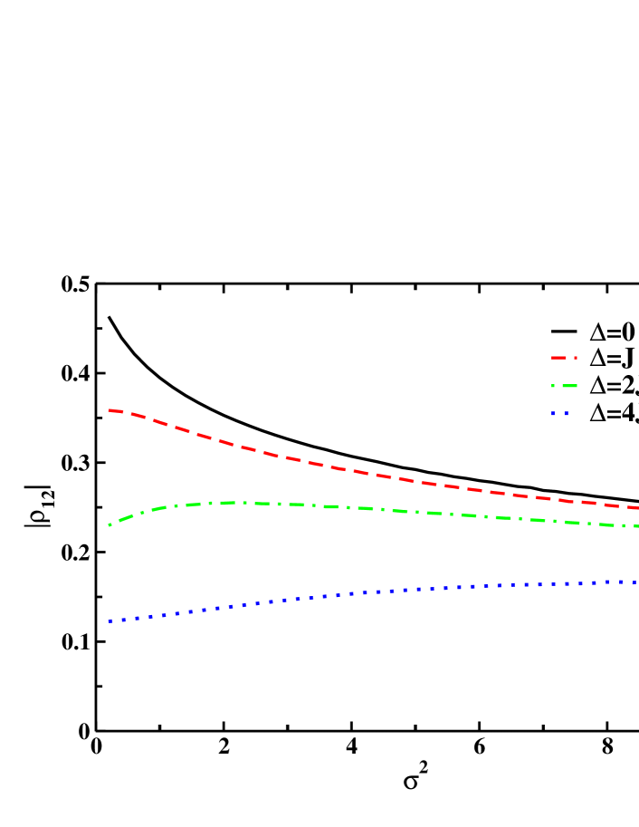
Figure 2: (color online) The off diagonal element of the density matrix calculated as a function of the variance of the static disorder distribution. In both cases $J=1$ and the temperature is fixed at $\beta=10$. The (green) dot-dashed line, (blue) dotted line, (red) dashed line, and (black) solid line correspond to detunings of the energy levels of $\Delta=4J$, $2J$, $J$, $0$, respectively.

The second interesting feature of Fig. 1(b) is that at low temperatures, increasing the width of static disorder may lead to an increase of $L_{\rho}$. This behavior is captured by either definition of the coherence length. For the two-level system, the coherence length is determined simply by the single off-diagonal element of the reduced density matrix. In Fig. 2, $\rho_{12}$ is shown as a function of the width of the static disorder distribution for various cases of the bias with a fixed inverse temperature of $\beta=10$. This temperature is sufficiently low such that it is only necessary to consider the off-diagonal element of the reduced density matrix at zero temperature. In this case, the disorder-averaged density matrix element is given by

$$\left|\rho_{12}\right|=\frac{J}{2}\left\langle\left[J^{2}+(\Delta+\epsilon)^{2}\right]^{-1/2}\right\rangle\;,$$ (28)

where the average is taken over the distribution of Gaussian disorder, $P(\epsilon)$ in Eq. 21 Only for the case of the symmetric two level system can $\rho_{12}$ be calculated exactly for which one obtains,

$$\left|\rho_{12}\right|=\frac{1}{\sqrt{2\pi\sigma^{2}}}e^{\frac{J^{2}}{4\sigma^{2}}}\frac{J}{2}K_{0}\left(\frac{J^{2}}{4\sigma^{2}}\right)\;,$$ (29)

where $K_{0}$ is the zero-order modified Bessel function of the second kind. This expression decreases monotonically with increasing width of the static disorder distribution as also seen from Fig. 1(a). That is, the introduction of disorder can only decrease the coherence length in the symmetric two level system.

Likewise, the two level system is maximally coherent also in the absence of bias. The presence of bias reduces $\rho_{12}$ by a factor of $J/\sqrt{J^{2}+\Delta^{2}}$ at low temperature. Provided that the ratio $J^{2}/\sigma^{2}$ is large, the initial increase in the coherence length of the biased two level system with increasing disorder seen in Figs. 2 and 1(b) may be computed from Eq. 28 as

$$\left|\rho_{12}\right|\approx\frac{J}{2\lambda}\left(1+\sigma^{2}\frac{2\Delta^{2}-J^{2}}{2\lambda^{4}}+O(\sigma^{4})\right)\;.$$ (30)

As can be seen from this expression, for $2\Delta^{2}>J^{2}$, there will be an initial increase in the magnitude of the off-diagonal element of the reduced density matrix, and hence also the coherence length.

The physical origin of the increase in the coherence length may be explained by realizing that the disorder gives rise to a distribution of site energies. The coherence length will be largest when the overlap of the two site energy distributions is maximized. It is easily seen for the symmetric two level system that this criterion implies that the coherence is largest only when the distribution of static disorder has zero width as seen in Figs. 1(a) and 2. However for the biased case, there will be an optimal width of the static disorder distribution that will increase the overlap of the two sites. This leads to a maximum in the coherence length at a non-zero value of the width of the static disorder distribution in biased systems as seen in Fig. 1(b). It will be seen below that many of these simple qualitative considerations regarding the coherence length in two level systems will also hold true in the more complicated settings of LH2 and FMO.

IV.2 LH2

IV.2.1 Reduced density matrix

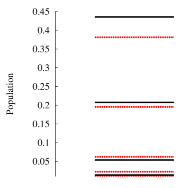
Figure 3: (color online) The Boltzmann populations (black) lines and the exact equilibrium populations (red) lines for the seven most populated states of LH2 at $300$ K. The lower three states are doubly degenerate. The thermal bath is modeled by the Ohmic spectral density described in Eq. 20 with a reorganization energy of $200$ cm^-1 and cutoff frequency of $100$ fs^-1.

In Ref. Strümpfer and Schulten, 2009, Strümpfer and Schulten presented the numerically exact time evolution of the exciton populations in LH2 obtained from the hierarchical equation of motion approach. They noted that the long time, steady state behavior of the exciton populations did not coincide with the those calculated from the Boltzmann populations of the bare system Hamiltonian. The difference is not entirely negligible; it lowers the population of the most lowest energy state by roughly $15\%$. Here we show that the steady state that is reached in the long time limit of their calculations is simply the true equilibrium state of the full system-bath Hamiltonian. In Fig. 3, the Boltzmann populations of the seven most populated exciton states (the lower three are doubly degenerate) are presented as well as the corresponding values obtained from the exact path integral calculations. The latter quantities are given by $P_{i}(\beta)=\left\langle\psi_{i}\right|\rho(\beta)\left|\psi_{i}\right\rangle$, where $\psi_{i}$ labels the $i$-th exciton basis function. The results in Fig. 3 are in excellent agreement with corresponding values presented in Ref. Strümpfer and Schulten, 2009. The difference between the populations calculated from the Boltzmann distribution and the reduced density matrix seen in Fig. 3 is an indication of the entanglement of the system and bath in the single excitation manifold. That is, the true equilibrium state for LH2 cannot be written as a product of independent system and bath states as is often assumed, even at room temperature. For example, in subsequent calculations of the energy transfer rate between two LH2 rings based up Forster theory, Strümpfer and Schulten noted that using the correct equilibrium distribution instead of the populations given by the Boltzmann distribution leads to a corresponding decrease in the transfer rate of approximately $10\%$. As will be demonstrated below, this correction becomes more important when either the temperature is lowered or the system-bath coupling increases.

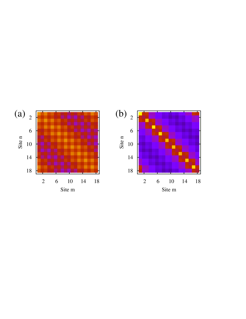
Figure 4: (color online) The absolute value of the density matrix elements $\left|\rho_{nm}\right|$ for LH2 at a temperature of $100$ K. The left is the Boltzmann distribution and the right is the exact reduced density matrix calculated at a reorganization energy of $600$ cm^-1.

In order to analyze the role of the environment in more detail, a comparison of the exact reduced density matrix and the approximate Boltzmann distribution at $100$ K is shown Fig. 4. In the absence of the thermal bath, the density matrix shown in Fig. 4(a) is almost completely delocalized. However, when the bath is included in Fig. 4(b), then the coherence length of the reduced density matrix is drastically reduced. Due to the circular arrangement of the chromophores in LH2, the Boltzmann density matrix must reflect the underlying symmetry of the Hamiltonian. The exact reduced density matrix must also preserve this symmetry since each of the independent thermal baths are identical. One important consequence of this result, for example, is that the exact reduced density matrix is diagonal in the exciton basis for any values of the temperature or bath parameters. An additional consequence of this symmetry is that all of the independent information contained in the density matrix for LH2 is captured by the elements of a single row or column. Therefore, these elements will be used to provide a more quantitative comparison for how the temperature and system bath coupling strength effect the localization length in LH2.

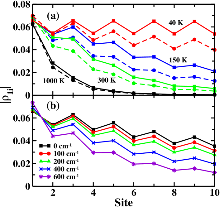
Figure 5: (color online) The density matrix elements $\rho_{1i}$ for LH2 versus the site number. In (a) the black, green, blue and and red lines correspond to temperatures of $1000$ K, $300$ K, $150$ K, and $40$ K with a fixed reorganization energy of $350$ cm^-1. The solid lines with squares are the values calculated from the Boltzmann distribution and the dashed lines with circles are the corresponding exact results from the path integral calculations. In (b) the (black) squares, (red) circles, (green) triangles, (blue) crosses and (purple) stars correspond to the Boltzmann distribution, and reorganization energies of $100$, $200$, $400$ and $600$ cm^-1, respectively, with a fixed temperature of $100$ K.

The first $10$ elements of the first row in the reduced density matrix are shown in Fig. 5(a) for four different temperatures with a constant reorganization energy of $350$ cm^-1 using the Ohmic spectral density. Perhaps surprisingly, at $1000$ K there is still some coherence present in LH2 as well as noticeable corrections to the Boltzmann distribution due to the bath. As the temperature is lowered, the density matrix becomes more delocalized as expected. However the corrections to the Boltzmann distribution due to the bath become more significant as well. Notice also that the difference between the Boltzmann results and the exact results is not systematic with increasing distance from the diagonal. For example, the largest difference between the Boltzmann and exact results shifts to larger site numbers as the temperature decreases. This fact prevents one from representing the exact density matrix simply as a Boltzmann distribution of the bare system with an effective temperature. The influence of the reorganization energy on the density matrix is shown in Fig. 5(b) at a fixed temperature of $100$ K. As the system bath coupling increases, the off-diagonal elements of the density matrix display a corresponding decrease. These two results in Fig 5(a) and (b) demonstrate that the system and bath are substantially entangled in the single exciton manifold for almost all physically relevant values of the environmental parameters. Treating the initial density matrix as a product state, as in generally done in most calculations of the dynamics in light harvesting systems, introduces an additional source of error that is not negligible, particularly at low temperatures.

IV.2.2 Coherence lengths in LH2

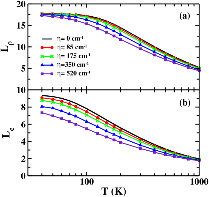
Figure 6: (color online) The coherence lengths, $L_{\rho}$ (a), and $L_{c}$ (b), calculated for LH2 as a function of temperature for increasing reorganization energy. The solid (black) line is obtained from the Boltzmann populations without noise. The reorganization energies of $85$, $175$, $350$, and $520$ cm^-1 are indicated by the (red) line with dots, (green) line with crosses, (blue) line with triangles, and (purple) line with squares, respectively. Note the increasing decay from the plateau at low temperatures.

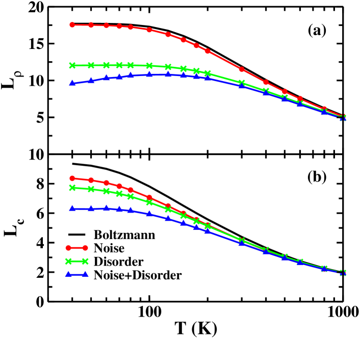
Figure 8: (color online) The coherence lengths, $L_{\rho}$ (a), and $L_{c}$ (b), calculated for LH2 as a function of temperature. The solid (black) line is obtained from the Boltzmann populations without noise or disorder. The (red) line with dots is obtained from calculations with noise only using the spectral density of Eq. 19, the (green) line with crosses is obtained from calculations with static disorder only with a width of $200$ cm^-1, and the (blue) line with triangles is from calculations with both noise and disorder.

While direct inspection of the density matrix provides the most unambiguous interpretation of the influence of the environment on the coherence length, it can become cumbersome for systems that lack the symmetry of LH2. As a result a variety of measures have been proposed to quantify the coherence length. They all provide some representation of the extent of the off-diagonal elements by assigning a single number for a given density matrix. It can already be seen from the above discussions that this distillation of information in the density matrix cannot be completely satisfactory. In this section we will compare two commonly used definitions for the coherence length. The influence of noise on the coherence length in LH2 is shown in Fig. 6 as a function of the temperature. The Ohmic spectral density is used here to assess how the reorganization energy effects the coherence length. Results for the spectral density of Ref. 19 are included below in Fig. 8. In the incoherent high temperature limit, the coherence length is 1 as expected since the density matrix is diagonal in this case. However, this limit is not reached until unphysically high values of the temperature. As was noted from the direct examination of the density matrices above in Fig. 5, as the temperature is lowered in the absence of noise, the coherence length gradually increases eventually reaching the respective maximal value in either measure. Likewise, increasing the strength of the system bath coupling generally leads to a decrease in the coherence length. There are, however, some significant differences between the two coherence length measures, particularly at low temperatures. In Fig. 6, $L_{\rho}$ shows very little dependence on the reorganization below $100$ K regardless of the strength of the noise, whereas $L_{c}$ steadily decreases with increasing reorganization energy. Compared with Fig. 5, $L_{c}$ seems to provide a more consistent reflection of the density matrix in this case.

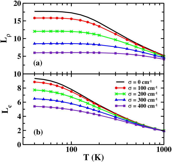
Figure 7: (color online) The coherence lengths, $L_{\rho}$ (a), and, $L_{c}$ (b), calculated for LH2 as a function of temperature for increasing static disorder. The solid (black) line is obtained from the Boltzmann populations without any static disorder. The widths of the static disorder distribution of $100$, $200$, $300$, and $400$ cm^-1 are indicated by the (red) line with dots, (green) line with crosses, (blue) line with triangles, and (purple) line with squares, respectively. Note the increasing persistence of the plateau with increasing disorder.

Aside from the role of homogeneous broadening, there is an additional source of decoherence in excitonic systems due to static disorder. The coherence lengths calculated for LH2 with static disorder are shown in Fig. 7. The width of the static disorder distribution was estimated to be $200$ cm^-1 in Ref. Strümpfer and Schulten, 2009, although estimates for this quantity vary widely. As static disorder is introduced into the system, the coherence length steadily decreases as expected from the above discussion for two level systems. Additionally the two different definitions for the coherence length display qualitatively similar behavior as has been observed before.Dahlbom et al. (2001) However, in contrast to the case of noise, at low temperatures $L_{\rho}$ now displays a stronger dependence on the disorder than $L_{c}$. Additionally, in both cases the coherence length reaches a plateau at low temperature. Such a feature is not formed in the case of the noise.

The affect of both noise and disorder on the coherence length in LH2 is shown in Fig. 8. Here the spectral density of the bath is taken as the form suggested by Olbrich et al in Eq. 19.Olbrich and Kleinekathöfer (2010) Qualitatively, the differences in the coherence lengths computed with this complicated spectral density and the simpler form used previously in Fig. 6 is rather small. The use of Eq. 19 leads to results that are quite similar to the Ohmic form used previously with a reorganization energy of between $200$ and $300$ cm^-1. The spectral density of Eq. 19 possess several strong peaks in the low frequency region which have been claimed to be essential in order to correctly describe the energy relaxation process in LH2.Adolphs and Renger (2006); van Grondelle and Novoderezhkin (2006); Olbrich and Kleinekathöfer (2010) Their influence on the coherence length, however, appears to be rather small. The real-time dynamics are more likely to exhibit a greater sensitivity to these components of the respective spectral densities. Results showing the effects of static disorder with a width of $200$ cm^-1 as was suggested in Ref. Strümpfer and Schulten, 2009 are also shown in Fig. 7. It is important to note that the combined effect of static disorder and thermal noise on the coherence length is not simply cumulative. This is particularly noticeable at low temperature in the case of $L_{\rho}$, but also for $L_{c}$. That is, both of these effects need to be properly accounted for in this regime in order to accurately describe the system.

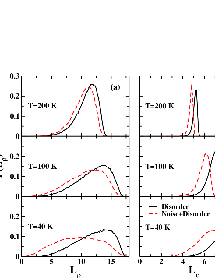
Figure 9: (color online) The distribution of the the coherence lengths, $L_{\rho}$ (a), and $L_{c}$ (b) for LH2. The top, middle and bottom panels correspond to temperatures of $200$, $100$ and $40$ K. The solid (black) lines represent the distributions obtained with static disorder only with a width of $200$ cm^-1. The dashed (red) lines display the results of disorder and noise using the spectral density of Eq. 19. Note the broadening induced by disorder and the shift that results from the noise.

To understand more clearly the difference between noise and disorder, the distribution of coherence lengths calculated with disorder alone, and with noise and disorder is shown in Fig. 9 at three different temperatures. The role of temperature, in general, provides the largest contribution to the coherence length distributions. At high temperatures, particularly for $L_{c}$, the distributions are quite sharp and neither disorder nor noise provide a significant contribution to the coherence length in this case. This is consistent with the small spread in coherence lengths seen above in Figs. 7 and 6 at high temperature for any values of the reorganization energy or disorder. The influence of static disorder is seen to both broaden the coherence length distributions as well as to introduce a skew towards lower values. These features become more pronounces at low temperatures. Including noise provides an additional constant shift of the whole coherence length distribution. The notable exception to this rule is the distribution of the $L_{\rho}$ at $40$ K where the presence of noise causes both a large shift and substantial change in the shape of the coherence length distribution. It is this effect which leads to the maximum as a function of temperature in Fig. 8. One also notes that there is little difference between the static disorder distributions of $L_{\rho}$ at $100$ and $200$ K. This accounts for the plateau in the coherence length distributions seen at low temperature in Fig. 7.

IV.2.3 Quenched and Annealed Disorder

Often in studies of light-harvesting systems, static disorder is said to arise from the very low frequency motions of the bath caused by large scale motions of the protein environment. However, this statement in inconsistent with the manner in which the calculations of static disorder are actually performed. Static disorder is due to the different local environments surrounding each of the chromophores. It leads different realizations of independent system Hamiltonians as occur, for example, in impurity models. The disorder that results from a very slow (adiabatic) bath, on the other hand, arises from internal degrees of freedom. The latter is a manifestation of annealed disorder, while the former is known as quenched disorder. It is generally accepted that the disorder present in light harvesting systems corresponds to the latter. Each sample of the static disorder corresponds to a physically realizable Hamiltonian as demonstrated by single molecule experiments. While the subtle difference between the two may seem only semantic, the consequences of this distinction can by quite significant. For example, annealed disorder implies that the system is ergodic and will (eventually) explore all possible bath configurations whereas quenched disorder corresponds to a system that is not ergodic.

An adiabatic bath can be easily considered within the formalism developed in Sec. II. This regime is obtained in the limit that the cutoff frequency of spectral density goes to zero. In this case, the dynamics of the bath degrees of freedom are much slower than that of the system. The kernel $K(\tau)$ in Eq. 8 then becomes independent of $\tau$ and may be replaced by a constant. The functional integral over the external field in Eq. 11 then reduces to a standard integral over a single Gaussian distribution with a fixed variance of the annealed disorder, $\sigma_{\rm ad}^{2}$. The final result of this procedure is that the reduced density matrix is given by $\hat{\rho}(\beta)=\langle e^{-\beta\hat{H}}\rangle/{\langle Z\rangle}$, where the angular brackets denote averaging with respect to the resulting Gaussian distribution of realizations of the slow bath. As with the case of general noise discussed above, the averaging here arises from tracing out the bath degrees of freedom. Contrast this situation with that of of quenched disorder in which one is led to the alternate expression for the reduced density matrix, $\hat{\rho}(\beta)=\langle e^{-\beta\hat{H}}/Z\rangle$. The averaging here is carried out over the distribution of Hamiltonians. It is clear that these two approaches are not equivalent. They lead to qualitatively different behavior at low temperatures.

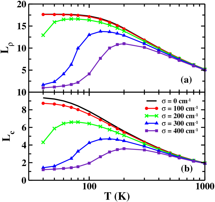
Figure 10: (color online) The coherence lengths $L_{\rho}$ (a), and $L_{c}$ (b), calculated for LH2 as a function of temperature for increasing strength of the annealed disorder. The solid (black) line is obtained from the Boltzmann populations without any disorder. The widths of the annealed disorder distribution of $100$, $200$, $300$, and $400$ cm^-1 are indicated by the (red) line with dots, (green) line with crosses, (blue) line with triangles, and (purple) line with squares, respectively.

The adiabatic bath model has been extensively analyzed in the context of the two-level system.Chandler (1991) In this model, there exists a critical value of the system parameters at which self trapping occurs. The system becomes localized when $\beta\sigma_{\rm ad}^{2}/J>1$, where $J$ is the coupling between the two levels.Chandler (1991) This transition persists for larger systems and is shown in Fig. 10 for LH2. Provided that the strength of the annealed disorder is greater than a critical value, there is a transition to a localized state at low temperature as indicated by the dramatic decrease seen in the coherence length measures. In contrast, the case of quenched disorder shown previously in Fig. 7 displayed the opposite behavior. There, both of the coherence length measures increased monotonically with decreasing temperature. It should be noted that a proper treatment of the limit of $K(\tau)$ for small $\omega_{c}$ leads a variance of the adiabatic bath that depends on both the temperature and reorganization energy. However, in order to be consistent with the treatment of static disorder and the analysis of Ref. Chandler, 1991, here we simply take $\sigma_{\rm ad}$ to be constant.

It is unlikely, however, that the adiabatic bath plays a large role in light harvesting systems as the migration of the exciton from one independent complex to another occurs on relatively fast time scales. Observing the effects of annealed disorder may be possible in other cases such as in extended J-aggregates where exciton lifetimes and diffusion lengths can be much longer than in light harvesting systems. It is known that the coherence length is related to both the superradiance and the Stokes shift at low temperatures. Observing transitions in these or other related quantities could be an indication that the slow bath fluctuations are non-negligible. Regardless of the implications, the static disorder which is most often referred to in discussions of light harvesting systems should not be described in terms of slow bath fluctuations.

IV.3 FMO

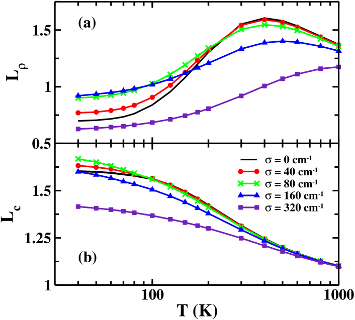
Figure 11: (color online) The coherence lengths $L_{\rho}$ (a) and $L_{c}$ (b), calculated for FMO as a function of temperature for increasing static disorder. The solid (black) line is obtained from the Boltzmann populations without any static disorder. The widths of the static disorder distribution of $40$, $80$, $160$, and $320$ cm^-1 are indicated by the (red) line with dots, (green) line with crosses, (blue) line with triangles, and (purple) line with squares, respectively.

Calculations of the coherence lengths performed for the FMO complex with static disorder are shown in Fig. 11. As with LH2, estimates for the width of the static disorder distribution vary widely although the value of $80$ cm^-1 has been used to fit several experimental results.Milder et al. (2010) The coherences lengths in FMO display behavior that is qualitatively different from those seen in LH2 in Fig. 7. Even without static disorder, neither of the coherence lengths continually increase to their respective maximal value as the temperature is lowered as was observed for LH2. Similar to the results presented for the biased two level system in Fig. 1, $L_{\rho}$ reaches a maximum value and then decreases as a function of the temperature. Additionally, at low temperatures it is seen that the static disorder can lead to an increase in the coherence length as was also observed in the biased two level system. As discussed previously, the peak in the $L_{\rho}$ and values less than one are an indication of the onset of localization at the lowest energy site. Direct inspection of the reduced density matrix confirms that this is the case. Regardless of the definition, both estimates yield rather small values for the coherence length that extends over one or two chromophores. As mentioned previously, FMO functions as an energy funnel in photosynthetic systems which efficiently transports energy from the antenna complex to the reaction center. Therefore, the equilibrium state will rarely be reached in this system. Nevertheless, FMO is considered here as simply a reasonable model for general disordered excitonic systems.

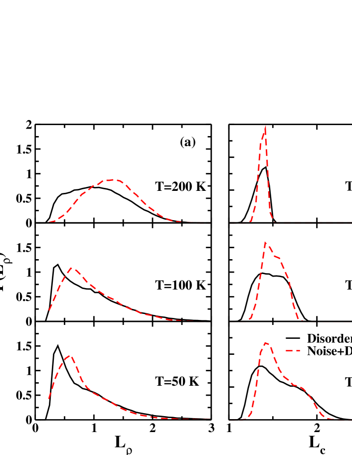
Figure 12: (color online) The distribution of the the coherence lengths, $L_{\rho}$ (a), and $L_{c}$ (b) for FMO. The top, middle and bottom panels correspond to temperatures of $200$, $100$ and $50$ K. The solid (black) lines represent the distributions obtained with static disorder only with a width of $80$ cm^-1. The dashed (red) lines display the results of disorder and noise with a reorganization energy of $35$ cm^-1.

The coherence length distributions of FMO calculated with both disorder and noise are shown in Fig. 12. As with the case of LH2, the temperature effect is seen to have the largest impact on the coherence length distributions. It has been noted above that the presence of disorder can increase the coherence length in FMO. Fig. 12 demonstrates that the addition of noise may increase the coherence length even further. In all cases, the distribution of noise and disorder compared with that of disorder alone is shifted to higher values of the coherence length. The origin of the maximum that is observed in Fig. 11(a) can be seen from the differences between the distributions of $L_{\rho}$ at $200$ K and $100$ K. At $100$ K, a significant portion of the distribution of coherence lengths is composed of values of $L_{\rho}$ less than $1$ which is indicative of localization on a single site.

V Concluding remarks

A general and efficient method for computing the exact equilibrium matrix for systems governed by a system-bath Hamiltonian was presented. This approach has several advantages over standard implementations of the imaginary time path integral approach. First, due to a Hubbard-Stratonovich transformation, the imaginary time convolution that appears in the influence functional is replaced by an additional functional integral over an auxiliary Gaussian field. The latter is readily amenable to a straightforward importance sampling Monte Carlo procedure. Additionally this allows one to compute the entire reduced density matrix from a single simulation, whereas in standard path integral treatments each element of the density matrix must be evaluated separately. As was demonstrated above, the simplicity and versatility of this approach allows for the treatment of both quenched and static disorder, as well as general thermal noise all within the same framework outlined in Sec. II.

Applying this technique, we presented exact results for the equilibrium reduced density matrix and the coherence lengths in FMO and LH2. For typical values of the system-bath coupling in these systems, it was demonstrated that the system and bath are entangled in the single exciton manifold, even at room temperature. As seen from Figs. 3 and 5, the exciton populations are only approximately given by a Boltzmann distribution of the bare system, and this approximation becomes progressively worse as the system-bath coupling increases and the temperature is lowered.

The role of static disorder, thermal noise and temperature on the coherence length was then systematically investigated for two commonly used measures of this quantity. Comparing Fig. 1 with Figs. 7 and 11 it is seen that the qualitative influence of static disorder on LH2 and FMO is well described by that of the respective symmetric and biased two level system. An extensive analysis for the latter was presented in Sec. IV.1. For symmetric systems, disorder only leads to a decrease in the coherence length, whereas in biased systems, disorder may increase the coherence length. There are some important differences between the role noise and disorder, particularly at low temperatures. For example, static disorder leads to a plateau in the coherence length that becomes increasingly pronounced with increasing strength of the disorder at low temperatures. The addition of thermal noise, however, can prevent this feature from occurring.Kamishima et al. (2007) The combined effect of both noise and disorder shown in Figs. 9 and 12 is different from either of them alone. In unbiased systems, increasing the temperature narrows the distribution of the coherence lengths, whereas static disorder leads to both broadening and skewing. The presence of noise results in an additional shift of the distribution towards the localization. However, for biased systems such as FMO, disorder can increase the coherence length, and the additional presence of noise may increase it further. Finally the influence of the environment as modeled either by static disorder or a slow bath was compared in Figs. 7 and 10. These two scenarios are not equivalent as is often claimed, and they lead to qualitatively different behavior at low temperature. Annealed disorder (a slow bath) leads to a sharp transition to localization at low temperature whereas quenched disorder does not.

While the two measures of the coherence length in Eqns. 23 and 24 provide the same qualitative picture of the effect of the environment on the coherence length at high temperatures, some significant differences appear in the low temperature regime. For biased systems such as FMO, $L_{\rho}$ shows a maximum in the coherence length as a function of temperature whereas $L_{c}$ does not. In symmetric systems, $L_{\rho}$ leads to a plateau in the coherence length at low temperatures that is much more pronounced than that of $L_{c}$. Additionally, $L_{\rho}$ predicts that LH2 is almost completely coherent at low temperatures regardless of the strength of the thermal noise. These qualitative differences should serve as a note of caution when using such coarse measures to characterize the coherence length in excitonic systems.

Due to the generality of the numerical scheme presented here, there are many possible extensions to this work. The application of this path integral technique to the study of the coherence length in larger systems such as J-aggregates, the chlorosome, and nanotubes is currently being investigated. In a forthcoming publication, the path-integral results provide a benchmark for various approximate methods including the polaron transformation and its variational form. Additionally, this approach can provide exact results for the thermal entanglement at finite temperatures in quantum information and quantum computing applications. Finally we mention the possibility of analytically continuing imaginary time correlation functions in order to obtain the corresponding real time quantities. For example, this would allow for the exact calculation of diffusion coefficients in rather large systems. These topics will be the focus of future publications.

VI Acknowledgments

We thank Johan Strümpfer for providing the crystal structure of LH2 needed for constructing the Hamiltonian used in this work. This work was supported by grants from the National Science Foundation (grant number CHE-1112825), DARPA, and the Center for Excitonics at MIT funded by the Department of Energy (grant number DE-SC0001088). Additionally, support from the Singapore National Research Foundation through the Competitive Research Programme (CRP) under Project No. NRF-CRP5-2009-04 is gratefully acknowledged. J Cao is supported as part of the Center of Excitonics, an Energy Frontier Research Center funded by the US Department of Energy, Officie of Science, Office of Basic Energy Sciences under Award No. DE-SC0001088.

Appendix A Discrete systems

The procedure leading to Eq. 15 in Sec. II is most easily generalized to discrete systems through the mapping formalism.Stock and Thoss (1997); Thoss and Stock (1999) In this approach, the discrete levels of the system Hamiltonian are mapped to continuous bosonic creation and annihilation variables through the relations, $\left|n\right\rangle\left\langle m\right|\rightarrow a_{n}^{\dagger}a_{m}$. The path integrals over the system and bath can then be constructed in a mixed representation using the usual coordinate states for the bath degrees of freedom and the coherent state representation for the bosonic modes. This approach has been successfully applied, for example, to model the dynamics of a two level system coupled to a dissipative vibrational degree of freedom.Novikov et al. (2004) The construction of the system action for the bosonic modes requires some care but is extensively discussed in Refs. Kleinert, 2004 and Su, 2000. However, as with the case of the continuous Hamiltonians discussed in the main text, the explicit form of the system action is never required. With these preliminaries, the procedure outlined in Sec. II proceeds identically. The influence functional follows the continuous form before except with the system coordinate $f(q)$ replaced by the proper coupling (generally it is one of the sites $a_{n}^{\dagger}a_{n}$), and the Hubbard-Stratonovich transformation in unaffected. At the end of the calculation one can map the bosonic variables back to the original discrete levels, and finally obtain the result of Eq. 15.

Appendix B FMO Hamiltonian

The Hamiltonian for FMO is taken from Ref. Cho et al., 2005. The specific values (in cm^-1) are given by

$$H_{\rm FMO}=\begin{pmatrix}280&-106&8&-5&6&-8&-4\\ -106&420&28&6&2&13&1\\ 8&28&0&-62&-1&-9&17\\ -5&6&-62&175&-70&-19&-57\\ 6&2&-1&-70&320&40&-2\\ -8&13&-9&-19&40&360&32\\ -4&1&17&-57&-2&32&260\end{pmatrix}\;.$$ (31)

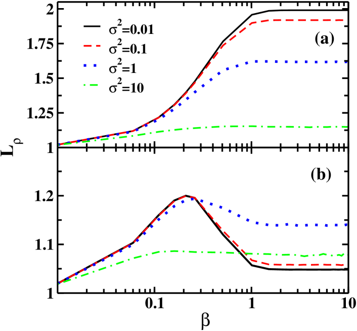
Figure 1: (color online) The effect of static disorder on $L_{\rho}$ calculated for the symmetric (top) and biased (bottom) two level system. In both cases $J=1$ and the detuning is $\Delta=2J$ biased case. The variance of the static disorder is $\sigma^{2}=10$ for the (green) dot-dashed line, $1$ (blue) dotted line, $0.1$ (red) dashed line and $0.01$ (black) solid line. Note the plateau at low temperatures in the symmetric case and the peak in (b).

References

- Kleinert (2004) H. Kleinert, Path Integrals in Quantum Mechanics, Statistics, and Polymer Physics, and Financial Markets (World Scientific, Singapore, 2004), 3rd ed.
- Schulman (1986) L. S. Schulman, Techniques and Applications of Path Integration (Wiley, New York, 1986).
- Feynman and Vernon (1963) R. P. Feynman and F. L. Vernon, Ann. Phys. (NY) 24, 118 (1963).
- Grabert et al. (1988) H. Grabert, P. Schramm, and G.-L. Ingold, Phys. Rep. 168, 115 (1988).
- Wu et al. (2010) J. Wu, F. Liu, Y. Shen, J. Cao, and R. J. Silbey, New J. Phys. 12, 105012 (2010).
- Wu et al. (2011) J. Wu, F. Liu, J. Ma, X. Wang, R. Silbey, and J. Cao (2011), submitted.
- Cho et al. (2005) M. Cho, H. M. Vaswani, T. Brixner, J. Stenger, and G. R. Fleming, J. Phys. Chem. B 109, 10542 (2005).
- Meier et al. (1997a) T. Meier, V. Chernyak, and S. Mukamel, J. Phys. Chem. B 101, 7332 (1997a).
- Meier et al. (1997b) T. Meier, Y. Zhao, V. Chernyak, and S. Mukamel, J. Chem. Phys. 107, 3876 (1997b).
- Monshouwer et al. (1997) R. Monshouwer, M. Abrahamsson, F. van Mourik, and R. van Grondelle, J. Phys. Chem. B 101, 7241 (1997).
- Potma and Wiersma (1998) E. O. Potma and D. A. Wiersma, J. Chem. Phys. 108, 4894 (1998).
- Chernyak et al. (1999) V. Chernyak, T. Meier, E. Tsiper, and S. Mukamel, J. Phys. Chem. A 103, 10294 (1999).
- Pullerits et al. (1996) T. Pullerits, M. Chachisvilis, and V. Sundström, J. Phys. Chem. 100, 10787 (1996).
- Kühn and Sundström (1997) O. Kühn and V. Sundström, J. Chem. Phys. 107, 4154 (1997).
- Ray and Makri (1999) J. Ray and N. Makri, J. Phys. Chem. A 103, 9417 (1999).
- Strümpfer and Schulten (2009) J. Strümpfer and K. Schulten, J. Chem. Phys. 131, 225101 (2009).
- Yakolev et al. (2002) A. Yakolev, V. Novoderezhkin, A. Taisova, and Z. Fetisova, Photosynth. Res. 71, 19 (2002).
- Cheng and Silbey (2006) Y. C. Cheng and R. J. Silbey, Phys. Rev. Lett. 96, 028103 (2006).
- Jang et al. (2001) S. Jang, S. E. Dempster, and R. J. Silbey, J. Phys. Chem. B 105, 6655 (2001).
- Dahlbom et al. (2001) M. Dahlbom, T. Pullerits, S. Mukamel, and V. Sundström, J. Phys. Chem. B 105, 5515 (2001).
- Prokhorenko et al. (2003) V. Prokhorenko, D. Steensgaard, and A. Holzwarth, Biophys. J. 85, 3173 (2003).
- Mülken et al. (2007) O. Mülken, V. Bierbaum, and A. Blumen, Phys. Rev. E 75, 031121 (2007).
- Fidder et al. (1991) H. Fidder, J. Knoester, and D. A. Wiersma, J. Chem. Phys. 95, 7880 (1991).
- Dijkstra et al. (2008) A. G. Dijkstra, T. la Cour Jansen, and J. Knoester, J. Chem. Phys. 128, 164511 (2008).
- Eisfeld et al. (2010) A. Eisfeld, S. M. Vlaming, V. A. Malyshev, and J. Knoester, Phys. Rev. Lett. 105, 137402 (2010).
- Vlaming et al. (2009) S. M. Vlaming, V. A. Malyshev, and J. Knoester, Phys. Rev. B 79, 205121 (2009).
- Kumble and Hochstrasser (1998) R. Kumble and R. M. Hochstrasser, J. Chem. Phys. 109, 855 (1998).
- Novoderezhkin et al. (1998) V. Novoderezhkin, R. Monshouwer, and R. van Grondelle, J. Phys. Chem. B 103, 10540 (1998).
- Ishizaki and Fleming (2010) A. Ishizaki and G. R. Fleming, New J. Phys. 12, 055004 (2010).
- Chandler (1991) D. Chandler, in Liquids, Freezing and the Glass Transition, Les Houches, edited by D. Levesque, J. P. Hansen, and J. Zinn-Justin (Elsevier, New York, 1991), p. 193.
- Cao et al. (1996) J. Cao, L. W. Ungar, and G. A. Voth, J. Chem. Phys. 104, 4189 (1996).
- Cao and Voth (1996) J. Cao and G. A. Voth, J. Chem. Phys. 105, 6856 (1996).
- Kamishima et al. (2007) O. Kamishima, B. Paxton, T. Feurer, K. A. Nelson, Y. Iwai, J. Kawamura, and T. Hattori, J. Phys.-Condens. Mat. 19, 456215 (2007).
- Weiss (1999) U. Weiss, Quantum Dissipative Systems (World Scientific, Singapore, 1999), 2nd ed.
- Sugiyama and Koonin (1986) G. Sugiyama and S. Koonin, Ann. Phys. 168, 1 (1986).
- Mak and Chandler (1991) C. H. Mak and D. Chandler, Phys. Rev. A 44, 2352 (1991).
- Stockburger and Grabert (2002) J. T. Stockburger and H. Grabert, Phys. Rev. Lett. 88, 170407 (2002).
- Shao (2004) J. Shao, J. Chem. Phys. 120, 5053 (2004).
- Makri (1998) N. Makri, J. Chem. Phys. 109, 2994 (1998).
- Olbrich and Kleinekathöfer (2010) C. Olbrich and U. Kleinekathöfer, J. Phys. Chem. B 114, 12427 (2010).
- Olbrich et al. (2011) C. Olbrich, J. Strümpfer, K. Schulten, and U. Kleinekathöfer, J. Phys. Chem. B 115, 758 (2011).
- Damjanović et al. (2002) A. Damjanović, I. Kosztin, U. Kleinekathöfer, and K. Schulten, Phys. Rev. E 65, 031919 (2002).
- Ishizaki and Fleming (2009) A. Ishizaki and G. R. Fleming, Proc. Natl. Acad. Sci. USA 106, 17255 (2009).
- Donehue et al. (2011) J. E. Donehue, O. P. Varnavski, R. Cemborski, M. Iyoda, and T. Goodson, J. Am. Chem. Soc. 133, 4819 (2011).
- Milder et al. (2010) M. T. W. Milder, B. Brüggemann, R. van Grondelle, and J. L. Herek, Photosynth. Res. 104, 257 (2010).
- Adolphs and Renger (2006) J. Adolphs and T. Renger, Biophys. J. 91, 2778 (2006).
- van Grondelle and Novoderezhkin (2006) R. van Grondelle and V. I. Novoderezhkin, Phys. Chem. Chem. Phys. 8, 793 (2006).
- Stock and Thoss (1997) G. Stock and M. Thoss, Phys. Rev. Lett. 78, 578 (1997).
- Thoss and Stock (1999) M. Thoss and G. Stock, Phys. Rev. A 59, 64 (1999).
- Novikov et al. (2004) A. Novikov, U. Kleinekathöfer, and M. Schreiber, Chem. Phys. 296, 149 (2004).
- Su (2000) J.-C. Su, Physics Letters A 268, 279 (2000).