Abstract

We examine the existence and stability of discrete spatial solitons in coupled nonlinear lasing cavities (waveguide resonators), addressing the case of active defocusing media, where the gain exceeds damping in the low-amplitude limit. A new family of stable localized structures is found: these are bright and grey cavity solitons representing the connections between homogeneous and inhomogeneous states. Solitons of this type can be controlled by the discrete diffraction and are stable when the bistability of homogenous states is absent.

OCIS codes:  190.1450, 190.4390, 190.4420

Due to the huge progress in semiconductor-based photonic devices, a multitude of experimentally achievable concepts have arisen, aimed at performing optical processing and light reconfiguration [2, 1]. One of these concepts relates to light manipulation in semiconductor microcavities closed by high-reflectivity Bragg reflectors (microresonators). The cavity medium consists typically of quantum well structures which can be absorbing or (with electrical or optical pumping) provide gain [1]. The soliton solutions in driven optical cavities (cavity solitons, CS) have attracted much attention because of their potential applications in information processing and optical memory schemes: The ability to control their switch-on/off process by an address beam, and their location by introducing gradients in the holding beam makes them interesting as mobile pixels for reconfigurable arrays of all-optical processing units [1]. The CS are a particular realization of the dissipative soliton notion – localized structures existing due to the balance between dissipation, nonlinearity and diffraction [2].

A relatively new direction in the light processing in optical cavities refers to coupled systems of microresonators [3, 4, 5, 6, 7, 8, 9] where the excitation level of each cavity (or of an ordered pattern) can serve as an elementary ’pixel’. These ’pixels’ are based on yet another type of dissipative solitary structures – the discrete cavity solitons (DCS), which are localized excitations in coupled arrays of nonlinear cavities. Achieving controlled manipulations with ’pixels’ requires a detailed study of the properties of these objects: nucleation thresholds, stability, mobility etc [3]. It has to be noted that, unlike the continuum case [1], the studies of DCS have so far only dealt with the case of a passive cavity, i.e. the losses were assumed to dominate over the lasing gain [4, 5, 6, 7, 8, 9]. At the same time there is an interesting idea of self-sustained light spots in cavities with active gain [1], where no external driving is needed for supporting the stability of the CS (pixels). Therefore additional efforts are needed to address specifically the case of DCS in active media.

In this Letter we, for the first time to our knowledge, consider the properties of DCS in coupled active cavities and demonstrate that their structure and stability can be drastically different from their counterparts in passive systems [3, 4, 5, 6, 7, 8, 9]. In addition, we show that by adjusting the coupling (which is an example of a discrete diffraction management) one can control the stability of the DCS (a similar idea for passive planar resonators was used in [10]) which can be implemented as a useful tool for all-optical processing in discrete systems.

We consider a regular array of evanescently coupled identical nonlinear cavities with high-reflectivity mirrors placed at their facets, driven by a homogeneous holding beam having a normal incidence. The mean-field model for the light distribution within the array can be derived from the coupled-mode equations [4] assuming that i) the frequency detuning from the cavity resonance is small (high-finesse cavities) and ii) the temporal dynamics is slow compared to the round-trip time, i.e. the structure is short compared to the coupling and nonlinearity lengths (an effective cavity length is on the order of 1-2$\mu$m, though much longer structures can also be fabricated [1]). Then the system of (normalized) equations governing the dynamics of the averaged beam amplitude inside the $n$-th cavity, $A_{n}$, reads as:

$$\Big{(}\!\!\!\!\!\! i \!\!\!\!\!\!\!\frac{d}{dt}+\Delta+\alpha|A_{n}|^{2}\Big{)}A_{n}+$$ (1)

$$+ \!\!\!\!\!\,C\big{(}A_{n+1}+A_{n-1}-2A_{n}\big{)}-iF(A_{n})=P,$$

where all coefficients are real, $C>0$ characterizes the coupling strength, $\tilde{\Delta}=\Delta-2C$ is the detuning of the pump frequency from the resonant one, $\alpha$ characterizes the strength of the nonlinear (Kerr) polarization, $P>0$ is the amplitude of the holding beam and $F(A_{n})$ describes dissipative effects. The field $A_{n}$ is normalized to the lasing saturation intensity $I_{0}$: $A_{n}/\sqrt{I_{0}}\to A_{n}$, and the time to the cavity round trip time (see also [4]).

The existence and stability properties of DCS in model (1) can be essentially different from those of the continuous counterparts [4, 3]. In this Letter we will specifically concentrate on highly discrete solutions occurring in the case of defocusing nonlinearity, $\alpha<0$, existing up to a limiting value of $C$ and having no continuum limit. We opt for a simple but physically important and general form of dissipative function with gain saturation [3, 7, 11]: $F(A_{n})=A_{n}[\gamma(1+|A_{n}|^{2})^{-1}-\delta]$, and the active region corresponds to amplitudes satisfying $F(|A|)>0$ (highlighted part of the horizontal axis in Figs.1, 3). Here parameters $\delta,\gamma>0$ describe linear losses and gain respectively. We will assume that in the low-power limit the system is active, so that $\gamma>\delta$, distinguishing the case considered here from other studies of DCS [3, 4, 5, 6, 7, 11, 8, 9]. This implies that in the absence of a holding beam ($P=0$) the trivial solution $A_{n}\equiv 0$ of Eq.(1) is unstable.

To specify the order of coefficients entering Eq.(1) we took parameters for GaAs semiconductor lasers [2] with the linear refractive index $n_{0}=3.55$, saturation intensity $I_{0}=10^{8}\,\mathrm{W/cm^{2}}$, the Kerr coefficient $n_{2}=-2~{}\times~{}10^{-13}~{}\mathrm{cm^{2}/W}$, the linear gain 1.5cm^-1 and the loss 0.5 cm^-1. Assuming the cross-section of resonators being $5\mu$m², we get that the unit of the normalized amplitude corresponds to the power $0.5$mW. The round trip frequency is $\Omega\sim 10~{}^{10}s^{-1}$. With this in mind we set all dimensionless coefficients $\Delta$, $\delta$, $\alpha$ and $\gamma$ in order of unity, which appears to be achievable in experiments. For the visualization of our results we opt for the following particular values: $\Delta=3.5$, $\delta=0.4$, $\gamma=1.7$, $\alpha=-0.2$, yielding $|A|<1.8$ as active region. For distances $\sim 1\div 10$$\mu$m the coupling strength varies in a large interval, so we can use a relatively weak realistic coupling $C=0.15$, a value which for the chosen set of parameters is slightly below the upper existence limit for the solutions found below.

The analysis of DCS in the system (1) starts from the identification of stable homogeneous (H) states that serve as a background for localized solutions [3, 4, 5, 6, 7]: setting $A_{n}=A$ (or $C=0$) in Eq.(1) one finds the so-called response curve $P(|A|)$, plotted in Fig.1(a) for the parameters chosen. The static state is stable when Eq.(1) linearized above it has no time-growing solutions. When two stable H-states coexist (thick solid parts marked H1 and H2 in Fig.1(a)), solitons for nonzero $C$ can generally be found as connections between these states [7]: the H1-H2-H1 connection for bright solitons, where the core intensity exceeds the background, or the H2-H1-H2 connection for grey solitons with a ’dent’ in the H2 ‘substrate’. In our case, as for passive systems [3, 4, 5, 6, 7], such stable DCS exist in a certain interval within the bistability region of H-states caused by the Kerr nonlinearity; an example of a stable bright soliton is given in Fig.2 (upper right pane). The major difference of H-states in the active case is the instability of the low-amplitude part of the H1-branch, so that, in contrast to passive systems [3, 4, 5, 6, 7], DCS formed by such H-states connections cannot be stable at low $P$ values.

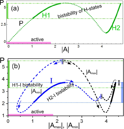
Fig. 1: (Color online.) Response curves for (a) homogeneous (H) and (b) 2-site periodic (I) solutions, with stable regions highlighted by thick solid lines. (a) $P(|A|)$ for H-solutions, with stable lower (H1) and higher (H2) states. (b) $P(|A_{max}|)$ and $P(|A_{min}|)$ for the I-solution; the direction of ‘evolution’ from the curve coalescence points (marked by $||$) is identified with arrows. Regions of H-H and H-I bistability are marked on the $P$-axes; the active region ($F(|A|)>0$) is highlighted on the $|A|$-axes.

Now we turn to another possible background for the formation of DCS – inhomogeneous periodic static state (we label it as an I-state). In general, infinitely many extended solutions with inhomogeneous patterning can be found but here, to demonstrate the main features introduced by coupling to the I-states, we deal with the simplest family having a 2-site period. Setting in Eq.(1) $A_{n},\,A_{n+2},\,\ldots=A_{max}$, and $A_{n+1},\,A_{n+3},\,\ldots=A_{min}$, $A_{max}\neq A_{min}$, we solve the system for these two complex fields. The results are given in Fig.1(b) in the form of two (equivalent) response curves: $P(|A_{max}|)$ and $P(|A_{min}|)$ (stable regions are marked with a thick solid line). The I-background is discrete and does not exist in the continuum limit $C\to\infty$. One can observe that the regions of stability for H-states and I-state partially overlap. This means that one can compose new families of localized solutions in the form of a fragment of the I-state embedded in a stable H-background (or vice versa). In addition, the I-state can be stable below the region of H-bistability, i.e. for parameters where one cannot have stable DCS in the form of H-states connections. Thus, in this region the only stable DCS represent connections of type H2-I.

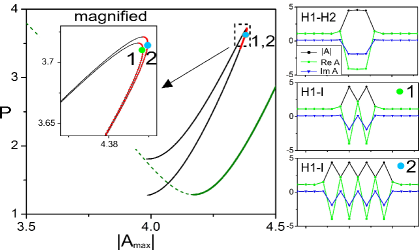
Fig. 2: (Color online.) Left pane: Snaking diagram for bright DCS corresponding to H1-I-H1 connection (stable regions are highlighted). The inset shows a magnified part of the snake. Right panes show particular field distributions for DCS: the top pane shows a stable DCS corresponding to the H1-H2-H1 connection ($P=4.3$), the two lower panes show the distributions for the stable DCS corresponding to H1-I-H1. The latter correspond to the points marked $\bullet$ ’1’, ’2’ on the snake.

In Figs. 2 and 3 we show examples of the new type of DCS corresponding to H-I connections found in our model. We present them on snaking diagrams where each point corresponds to a particular DCS. The bright/grey DCS are characterized by the maximal/minimal amplitude of the soliton so the snakes corresponding to each soliton type are plotted on the curves $P(|A_{max}|)$, (Fig.2, corresponding to H1-I-H1 connection) and $P(|A_{min}|)$, (Fig.3, H2-I-H2 connection). These DCS are discrete, i.e. they can exist only up to a finite value of coupling.

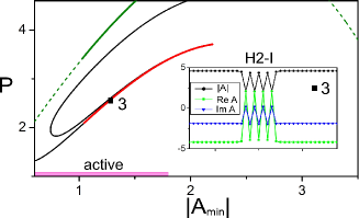
Fig. 3: (Color online.) Snaking diagram $P(|A_{min}|)$ for the grey DCS corresponding to the H2-I-H2 connection. The inset shows the particular distribution of stable DCS referring to the point marked as $\blacksquare$  ’3’.

They have a nonuniform central excited part corresponding to a fragment of the I-state embedded into either H1 or H2 background. Importantly, the grey DCS of this type can be stable in the region where no solitons representing the connections of H-states can be stable (see Fig.3), so this stability is achieved solely by the discrete diffraction. The solitons outside the stable regions typically display nonoscillatory exponential growth of small perturbations.

We note that, to the best of our knowledge, the DCS with H-I connections of the type found above have not been studied in works on (passive) coupled cavity systems, although a solution involving connections with a more complicated I-state was mentioned in [7]. Solutions involving oscillatory patterns at the tails were discussed in [8, 9]: in [8] DCS with oscillatory decaying tails were found, while in [9] the staggering low-amplitude plane-wave served as a background I-state for a grey DCS. Notably, both these types of DCS could be stable out of the H-bistability region. Our solutions have the staggering in the middle and come from the anticontinuous limit with generally large staggering oscillations. By decreasing $\gamma$ we checked that stable analogues of the H-I type DCS with a 2-periodic I-state in fact do exist also for passive systems.

Our findings have several important physical consequences. First, we have demonstrated that in active cavities, aside from ’traditional’ DCS representing connections between H-states, there can be stable solitary solutions with a lower power corresponding to the H-I connections, Figs.2, 3. Thus exerting an address beam for the nucleation of a ’pixel’ one can end up with an H-I rather than an H-H soliton. In turn, the mobility characteristics [9] of H-I solitons are likely to be different from those of the well-studied H1-H2 solutions, and the conditions for optical processing can significantly deviate from those of the ’conventional’ H-H DCS. Second, by adjusting the discrete diffraction (i.e. coupling) one can gain stable solitary solutions in the region of parameters, where no stable H1-H2 DCS can exist. Such stability control via a simple discrete diffraction management can be used as an additional tool for light manipulation: one can control not only the stability, but also the geometry of DCS providing more versatility for optical processing. Finally, the only stable type of DCS suitable for ’pixels’ manipulations in active cavities at low $P$ values (or for a relatively high gain) corresponds to the H-I solitons.

A.Y. and M.J. thank NCRG, Aston University, for kind hospitality. M.J. also acknowledges support from the Swedish Research Council. A.Y. was supported by the FCT (Portugal), grant PTDC/FIS/112624/2009.

Informational Fourth Page

In this section, please provide full versions of citations to assist reviewers and editors (OL publishes a short form of citations) or any other information that would aid the peer-review process.

References

- [1] T. Ackemann, W.J. Firth and G.-L. Oppo, in “Advances In Atomic Molecular and Optical Physics,” E. Arimondo, P.R. Berman and C.C. Lin (Eds.), vol. 57, 323 (2009).
- [2] “Dissipative Solitons,” N. Akhmediev and A. Ankiewicz (Eds.), Series: Lecture Notes in Physics, Vol. 661, (Springer: Berlin, Heidenberg), 2005.
- [3] F. Lederer, G.I. Stegeman, D.N. Christodoulides, G. Assanto, M. Segev, and Y. Silberberg, Phys. Rep. 463, 1 (2008).
- [4] U. Peschel, O. Egorov, and F. Lederer, Opt. Lett. 29, 1909 (2004).
- [5] O. Egorov, F. Lederer, and K. Staliunas, Opt. Lett. 32, 2106 (2007).
- [6] A.V. Yulin, A.R. Champneys, and D.V. Skryabin, Phys. Rev. A 78, 011804(R) (2008).
- [7] A.V. Yulin and A.R. Champneys, SIAM J. Appl. Dynam. Syst. 9, 391 (2010).
- [8] O. Egorov, U. Peschel, and F. Lederer, Phys. Rev. E 71, 056612 (2005).
- [9] O.A. Egorov, F. Lederer and Y.S. Kivshar, Opt. Express 15, 4149 (2007).
- [10] K. Staliunas, O. Egorov, Y.S. Kivshar, and F. Lederer, Phys. Rev. Lett. 101, 153903 (2008).
- [11] Al. S. Kiselev, An. S. Kiselev, and N. N. Rozanov, Opt. Spectrosc. 105, 547 (2008).

References

- [1] T. Ackemann, W.J. Firth and G.-L. Oppo, in “Advances In Atomic Molecular and Optical Physics,” E. Arimondo, P.R. Berman and C.C. Lin (Eds.), vol. 57, 323-421, 2009.
- [2] “Dissipative Solitons,” N. Akhmediev and A. Ankiewicz (Eds.), Series: Lecture Notes in Physics, Vol. 661, (Springer: Berlin, Heidenberg), 448 p., 2005.
- [3] F. Lederer, G.I. Stegeman, D.N. Christodoulides, G. Assanto, M. Segev, and Y. Silberberg, “Discrete solitons in optics”, Phys. Rep. 463, 1-126 (2008).
- [4] U. Peschel, O. Egorov, and F. Lederer, “Discrete cavity solitons”, Opt. Lett. 29, 1909-1912 (2004).
- [5] O. Egorov, F. Lederer, and K. Staliunas, “Subdiffractive discrete cavity solitons”, Opt. Lett. 32, 2106-2109 (2007).
- [6] A.V. Yulin, A.R. Champneys, and D.V. Skryabin, “Discrete cavity solitons due to saturable nonlinearity,” Phys. Rev. A 78, 011804(R) (2008).
- [7] A.V. Yulin and A.R. Champneys, “Discrete Snaking: Multiple Cavity Solitons in Saturable Media,” SIAM J. Appl. Dynam. Syst. 9 391-431 (2010).
- [8] O. Egorov, U. Peschel, and F. Lederer, “Discrete quadratic cavity solitons”, Phys. Rev. E 71, art.no 056612 (2005).
- [9] O.A. Egorov, F. Lederer and Y.S. Kivshar, “How does an inclined holding beam affect discrete modulational instability and solitons in nonlinear cavities?”, Opt. Express 15, 4149-4158 (2007).
- [10] K. Staliunas, O. Egorov, Y.S. Kivshar, and F. Lederer, “Bloch Cavity Solitons in Nonlinear Resonators with Intracavity Photonic Crystals,” Phys. Rev. Lett. 101, art.no 153903 (2008).
- [11] Al. S. Kiselev, An. S. Kiselev, and N. N. Rozanov, “Dissipative Discrete Spatial Optical Solitons in a System of Coupled Optical Fibers with the Kerr and Resonance Nonlinearities”, Opt. Spectrosc. 105, 547-556 (2008).