Conserved mass models with stickiness and chipping

Abstract

We study a chipping model in one dimensional periodic lattice with continuous mass, where a fixed fraction of the mass is chipped off from a site and distributed randomly among the departure site and its neighbours; the remaining mass sticks to the site. In the asymmetric version, the chipped off mass is distributed among the site and the right neighbour, whereas in the symmetric version the redistribution occurs among the two neighbours. The steady state mass distribution of the model is obtained using a perturbation method for both parallel and random sequential updates. In most cases, this perturbation theory provides a steady state distribution with reasonable accuracy.

Keywords: Transport processes, Stationary states, Solvable lattice models.

1 Introduction :

Most systems in nature are in non-equilibrium states [1], in a way that the accompanying fluxes of mass, energy, or spin etc. are irreversible. Unlike their equilibrium counterparts where the stationary state is characterized by the Gibbs measure, these systems usually reach different and novel stationary states depending on the dynamics of the microscopic constituents. Several non-equilibrium lattice models have been proposed recently [2] to investigate the unusual steady state distributions, spatio-temporal correlations and possibility of macroscopic collective phenomena.

One of the simple non-equilibrium models is the mass transport model where each site of a lattice is associated with discrete mass (particles) following a dynamics that involves aggregation, fragmentation, adsorption or desorption [3]. Like the zero range process [4], interestingly, many of these model systems undergo a condensation phase transition as the mass density of the system is increased. Study of these models have generated considerable interest among physicists, as a wide variety of systems exhibit basic microscopic mechanism similar to that of the simple mass transport models. These include colloidal suspensions [5], polymer gels [6], river networks [7], traffic models [8], and wealth distribution [9] etc.

A continuous version of the mass transport model is proposed recently [10] and some of its variations have also been studied [11, 12, 13]. Many of the mass transport models are known to evolve into a non-equilibrium steady state that has product measure. A generic criterion for factorized steady state has been derived [12, 13] for mass transport models. In our effort to study models where the steady state is not factorized and only a little is known analytically, we develop a perturbation approach that provides an approximate form of the steady state distribution.

In this article we introduce stickiness, quantified by a parameter $\lambda,$ to the continuous mass transport models. At each site, $(1-\lambda)$ fraction of the mass is chipped off (thus $\lambda$ fraction of the mass sticks to the site), which is then redistributed either asymmetrically, i.e. among the departure site and its right neighbour, or symmetrically, i.e. among the two neighbours. Accordingly, the model is referred to as asymmetric or symmetric sticky chipping model respectively. We use a novel perturbation approach to calculate the steady state mass distribution of these models, for both parallel and random sequential updates. Although in this perturbation approach, we have ignored two and three point spatial correlations, the mass distributions calculated up to $2^{nd}$ order are strikingly close to the same obtained from Monte Carlo simulations.

The article is organized as follows. The model and the perturbation method are outlined in section 2. In section 3 we study the asymmetric version of the model and obtain the steady state distribution. The symmetric version of the model, where the chipped off mass is distributed among both the neighbours, is discussed in section 4. Finally we discuss the main results in section 5. The perturbation results up to second order for all these models are listed in the Appendix.

2 The Model :

The model is defined on a one dimensional periodic lattice with sites labeled by $i=1,2,\dots,L$. A continuous mass $x_{i}$, associated at each site $i,$ evolves according to the following dynamics. At each site $i$, $(1-\lambda)$ fraction of the mass is chipped off (thus, $\lambda$ fraction of the mass sticks to the site) and then it is distributed among the departure site $i$ and its neighbours $(i\pm 1).$ In this article we study two different versions; in the asymmetric sticky chipping model (ASCM) the chipped off mass $(1-\lambda)x_{i}$ is distributed randomly among the sites $i$ and $(i+1),$ whereas in the symmetric sticky chipping model (SSCM) it is distributed among the neighbours $(i+1)$ and $(i-1)$. Both these versions are studied using parallel and random sequential update rules.

We must mention that the steady state mass distribution of ASCM with $\lambda=0$ has been obtained earlier by Rajesh $et.al.$ [10] assuming that the steady state is factorized. This product measure assumption turns out to be exact in case of parallel update and an excellent approximation (though not exact) in the random sequential case. We will show that in presence of stickiness $(\lambda\neq 0),$ neither ASCM nor SSCM can have a factorized steady state. To construct the steady state mass distribution $P(x)$, we use a novel perturbation approach. Although the spatial correlations are ignored here, the steady state distributions, calculated up to $2^{nd}$ order in $\lambda,$ are found to be in excellent agreement with the same obtained from the Monte Carlo simulations. The general principle of this approach is described in the following subsections.

2.1 Perturbation approach I :

We try to construct the steady state mass distribution $P(x)$ perturbatively, by expressing $P(x)$ as a power series in $\lambda,$ about $\lambda=0$ ,

$$P(x)=P_{0}(x)+\lambda P_{1}(x)+\lambda^{2}P_{2}(x)+\ldots=\sum_{k=0}^{\infty}\lambda^{k}P_{k}(x)$$ (1)

where the functions $P_{k}(x)$ do not depend on $\lambda$. Here we have omitted the argument $\lambda$ in $P(x)$ for notational convenience. The perturbative expansion can also be made about any other $\lambda$ if $P_{0}(x)$ can be calculated there. In the chipping models discussed here, the total mass of the system and hence the density $\langle x\rangle=\frac{1}{L}\sum_{i}x_{i}$ is conserved. Without any loss of generality one can fix the average mass to be unity. This imposes a condition on $P(x)$

$$\int_{0}^{\infty}dx~{}xP(x)=\langle x\rangle=1=\int_{0}^{\infty}dx~{}P(x)~{},$$ (2)

where the last equality stands for the normalization condition. Now, for $\lambda=0$, $P(x)=P_{0}(x)$. Therefore, $P_{0}(x)$ satisfies two conditions,

$$\int_{0}^{\infty}dx\ P_{0}(x)=1~{}{\rm and}\int_{0}^{\infty}dx\ xP_{0}(x)=1.$$ (3)

Thus for any other $k>0,$ using Eqs. (2) and (3) we have

$$\int_{0}^{\infty}dx\ P_{k}(x)=0=\int_{0}^{\infty}dx\ xP_{k}(x).$$ (4)

The above constraints can not be satisfied by any real positive function (as $x\geq 0$), and thus one can not interpret $P_{k}(x)$ as a probability density function.

The perturbative corrections $P_{k}(x)$ can be obtained directly from knowing the moments of $P(x)$. First let us expand the moments $\langle x^{n}\rangle=\int_{0}^{\infty}dx\ x^{n}P(x)$ as a power series in $\lambda$,

$$\frac{\langle x^{n}\rangle}{(n+1)!}\equiv A^{(n)}=\sum_{k=0}^{\infty}\lambda^{k}A_{k}^{(n)}.$$ (5)

Here $A_{k}^{(n)}$ are constant coefficients (independent of $\lambda$). The usefulness of the factor $1/(n+1)!$, used here for notational convenience, will be clear as we discuss specific problems. $A_{k}^{(n)}$ can be determined from Eqs. (1) and (5),

$$A_{k}^{(n)}=\frac{1}{(n+1)!}\int_{0}^{\infty}dx\ x^{n}P_{k}(x).$$ (6)

Since $P_{k}(x)$ are constrained by Eqs. (3) and (4) $A_{k}^{(n)}$ must satisfy,

$$A_{0}^{(1)}=\frac{1}{2}~{}~{}{\rm and}~{}~{}A_{k}^{(1)}=0~{}~{}\forall~{}~{}k>0.$$ (7)

Once $A_{k}^{(n)}$ are known, one can calculate $P_{k}(x)$ as

$$P_{k}(x)=\mathscr{L}^{-1}\left[\sum_{n=0}^{\infty}(-s)^{n}(n+1)A_{k}^{(n)}\right],$$ (8)

where $\mathscr{L}^{-1}$ denotes the inverse Laplace transform.

2.2 Perturbation approach II :

Here we assume that the mass distribution $P(x)$ satisfies a differential or an integral equation and use the Laplace transform

$$Q(s)=\mathscr{L}\left[P(x)\right]=\int_{0}^{\infty}dx\ e^{-sx}P(x)$$ (9)

which usually converts it into a differential or a transcendental equation in $Q(s).$ We proceed further by expanding $Q(s)$ as power series in $\lambda$ about $\lambda=0$,

$$Q(s)=\sum_{k=0}^{\infty}\lambda^{k}Q_{k}(s),$$ (10)

and equate the coefficients of different powers of $\lambda$ order by order. Finally one can find the distribution

$$P(x)=\mathscr{L}^{-1}\left[Q(s)\right]=\mathscr{L}^{-1}\left[\sum_{k=0}^{\infty}\lambda^{k}Q_{k}(s)\right].$$ (11)

These two approaches are equivalent as it is evident from Eq. (8),

$$Q_{k}(s)=\mathscr{L}\left[P_{k}(x)\right]=\sum_{n=0}^{\infty}(-s)^{n}(n+1)A_{k}^{(n)};$$ (12)

for any particular problem we will use the approach whichever is convenient.

3 Asymmetric Sticky Chipping Model (ASCM) :

In this section we study the asymmetric version of the model where $(1-\lambda)$ fraction of mass $x_{i}$ at site $i$ is chipped off, only $r_{i}$ fraction of the chipped off mass is then transported to the right neighbour $(i+1)$ and the rest is retained at site $i.$ In other words, from the site $i,$ $(1-\lambda)r_{i}$ fraction of the mass is transported to $(i+1).$ Here $r_{i}$ is a random number uniformly distributed in the interval $(0,1)$.

This asymmetric sticky chipping model can be mapped to the generic one dimensional mass transport models discussed in Ref. [12], by considering that the amount of mass $\mu$ that is transported from a site to its right neighbour is stochastic and distributed as

$$\phi(\mu|x)=\left\{\begin{array}[]{l l}\frac{1}{(1-\lambda)x}&0<\mu<(1-\lambda)x{\rm}\cr 0&{\rm otherwise}\end{array}\right.$$ (13)

where $x$ is the initial mass of the departure site. It has been shown [12] that the steady state mass distribution $P_{s}(\{x_{i}\})$ of the generic model is factorized, $i.e.~{}P_{s}(\{x_{i}\})=\prod_{i}f(x_{i}),$ only if $\phi(\mu|x)$ has the following form,

$$\phi(\mu|x)=\frac{v(\mu)w(x-\mu)}{f(x)},$$ (14)

where $v$ and $w$ are arbitrary functions and

$$f(x)=\left\{\begin{array}[]{l l}\int_{0}^{x}d\mu~{}v(\mu)w(x-\mu)&{\rm parallel~{}~{}update}\cr w(x)&{\rm random~{}~{}sequential~{}~{}update.}\end{array}\right.$$ (15)

It is evident from Eqs. (14) and (15) that models with parallel update can have a factorized steady state only if the dynamics remain invariant when $(x-\mu)$ is transported instead of $\mu.$ For ASCM, however, $(x-\mu)$ is distributed uniformly in the range $(\lambda x,x)$ (which is different from the range of $\mu$ in Eq. (13)) and thus the model can not have a factorized steady state for parallel update unless $\lambda=0.$ For random sequential update, Eqs. (13) and (15) suggest that $f(x)=w(x)\sim x$; but this can not be made consistent with Eq. (14) for any choice of $v.$ Thus random sequential update can not give a factorized steady state for any $\lambda$ (including $\lambda=0$).

In next two subsections we show that the mass distribution $P(x),$ calculated perturbatively, matches reasonably well with the same obtained from Monte Carlo simulations.

3.1 Parallel Update :

First let us consider the model with parallel update, where all the sites are updated synchronously. The dynamics can be written as

$$x_{i}(t+1)=\lambda x_{i}(t)+(1-\lambda)(1-r_{i})x_{i}(t)+(1-\lambda)r_{i-1}x_{i-1}(t)$$ (16)

for all $i=1,2,\dots,L,$ where the first term on r.h.s. represents the mass that sticks to the site $i,$ the second term corresponds to the mass that is retained at the site $i$ after $(1-\lambda)r_{i}x_{i}(t)$ is transported to $(i+1)$. The third term results from the mass that $i^{th}$ site receives from $(i-1)$.

This model has a factorized steady state for $\lambda=0$ as the distribution of transferred amount $\phi(\mu|x)=1/x$ (from Eq. (13)) can be written in the form suggested by Eq. (14) with $v(x)=1=w(x).$ Correspondingly $f(x)=x,$ which results in $P(x)=4xe^{-2x}.$ This special case of the model has been studied earlier by Rajesh $et.al.$ [10]. For any non-zero $\lambda,$ however, the steady state is not factorized.

In order to find the steady state mass distribution $P(x)$ for generic $\lambda$ first we calculate the moments. In the steady state, distribution of $x_{i}(t+1)$ is same as the distribution of $x_{i}(t)$. Thus, one may obtain $A^{(n)}\equiv\frac{\langle x^{n}\rangle}{(n+1)!}$ from Eq. (16) as

$$A^{(n)}=\left[n\bar{\lambda}-\lambda+\lambda^{n+1}-\bar{\lambda}^{n+1}\right]^{-1}\sum_{k=1}^{n-1}(1-\lambda^{k+1})\bar{\lambda}^{n-k}A^{(k)}A^{(n-k)}~{}~{}~{}~{}\forall~{}n\geq 2,$$

(17)

where we have used $\langle x_{i}^{m}x_{i-1}^{n}\rangle=\langle x_{i}^{m}\rangle\langle x_{i-1}^{n}\rangle,$ a mean field approximation that neglects all two point spatial correlations, and $\bar{\lambda}=(1-\lambda).$ Since $A^{(n)}$ depends on all other $A^{(k)}$ with $k=1,2,\dots,(n-1),$ it is usually difficult to get a general expression for $A^{(n)}$ from this recursion relation. However, it is evident from Eq. (17) that if $y(n)$ is a solution for $A^{(n)},$ $y(n)z^{n}$ is also a solution for any arbitrary $z.$ The arbitrary constant $z$ must be chosen such that the average mass of the system has the desired value $\langle x\rangle=1$ or in other words $A^{(1)}=\frac{1}{2}.$

First let us take $\lambda=0.$ In this case Eq. (17) reduces to a very simple form

$$A^{(n)}=\frac{1}{n-1}\sum_{k=1}^{n-1}A^{(k)}A^{(n-k)}~{}~{}~{}~{}~{}~{}\forall~{}n\geq 2,$$ (18)

which can be solved trivially by taking $A^{(n)}=1;$ thus a general solution is $A^{(n)}=z^{n}.$ The boundary condition $A^{(1)}=\frac{1}{2}$ now fixes $z=\frac{1}{2}$ and thus $\langle x^{n}\rangle=\frac{(n+1)!}{2^{n}}.$ Corresponding steady state distribution function is then

$$P(x)=\mathscr{L}^{-1}\left[\sum_{n=0}^{\infty}\frac{(-s)^{n}}{n!}\langle x^{n}\rangle\right]=4xe^{-2x}.$$ (19)

For generic $\lambda,$ $\langle x^{n}\rangle$ can be calculated recursively using Eq. (17) starting from $\langle x\rangle=1.$ The first few of them are,

$$\langle x^{2}\rangle=\frac{3(\lambda+1)}{4\lambda+2}$$ (20)

$$\langle x^{3}\rangle=\frac{3\left(\lambda^{2}+3\lambda+2\right)}{2(2\lambda+1)^{2}}$$ (21)

$$\langle x^{4}\rangle=\frac{15(\lambda+1)^{2}\left(\lambda^{2}-\lambda+3\right)}{2(2\lambda+1)^{2}\left(2\lambda^{3}-\lambda^{2}+6\lambda+3\right)}$$ (22)

$$\vdots.$$ (23)

The moments $\langle x^{n}\rangle$ as a function of $\lambda$ become messy with increasing $n$; obtaining a general expression for $\langle x^{n}\rangle$, and hence the distribution $P(x)$, becomes practically impossible. It would be useful to obtain $P(x)$ perturbatively which gives all the moments correctly (within this mean field approximation) up to some $n^{th}$ order in $\lambda$.

To proceed with the perturbation approach, we first express $\langle x^{n}\rangle$ in a power series in $\lambda$ as in Eq. (5) and then equate the coefficients of different powers of $\lambda$ which gives a set of recursion relations for $A^{(n)}_{k}.$ The recursion relation for any $n^{th}$ order perturbation in $\lambda$ can be solved using the boundary condition (7). Once $A^{(n)}_{k}$ are known, we calculate $P_{k}(x)$ using Eq. (8).

In the $0^{th}$ order, Eqs. (17) and (5) result in

$$A_{0}^{(n)}=\frac{1}{n-1}\sum_{k=1}^{n-1}A_{0}^{(k)}A_{0}^{(n-k)}~{}~{}~{}~{}~{}~{}\forall~{}n\geq 2,$$ (24)

which is indeed same as Eq. (18). Thus to this order, as expected, we get

$$A^{(n)}_{0}=\frac{1}{2^{n}},~{}~{}{\rm and}~{}~{}~{}P_{0}(x)=4xe^{-2x}.$$ (25)

Next we proceed to calculate the $1^{st}$ order correction to $P(x).$ Comparing the coefficients of $\lambda$ in Eq. (17) we have

$$A_{1}^{(n)}=\frac{1}{n-1}\sum_{k=1}^{n-1}[2A_{0}^{(k)}A_{1}^{(n-k)}-(n-k)A_{0}^{(k)}A_{0}^{(n-k)}]~{}~{}~{}~{}~{}~{}\forall~{}n\geq 2$$

which is needed to be solved using the boundary condition $A_{1}^{(1)}=0$, from Eq. (7). This results in

$$A_{1}^{(n)}=\frac{n}{2^{n}}\Big{(}1-\gamma-\frac{\Gamma^{\prime}(n+1)}{\Gamma(n+1)}\Big{)}~{}~{}~{}~{}~{}~{}\forall~{}n\geq 0$$ (26)

where $\Gamma(x)$ stands for usual gamma function and $\gamma$ is the Euler constant,

$$\gamma=0.57721\dots~{}~{}~{}.$$ (27)

Finally, using Eq. (8) we get

$$P_{1}(x)=8e^{-2x}\left[x^{2}\Big{(}1-g(x)\Big{)}+xg(x)-\frac{1}{4}\right]$$ (28)

$$\mbox{where}~{}g(x)=\ln(2x)+\gamma.$$ (29)

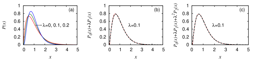
Figure 1: Steady state mass distribution $P(x)$ of ASCM with parallel update : (a) $P(x)$ obtained from Monte Carlo simulations of the system of size $L=1000$, for $\lambda=0,0.1,$ and $0.2$. (b) and (c) compare $P(x)$ for $\lambda=0.1$ with the $1^{st}$ and $2^{nd}$ order perturbation results (dashed line) respectively.

One can proceed in a similar way to calculate higher order corrections to $P(x).$ The corrections up to $2^{nd}$ order in $\lambda$ are listed in the Appendix.

To check that the perturbation results for $P(x)$ agree well with the actual steady state mass distribution we simulate the model on a one dimensional lattice of size $L=1000$ for $\lambda=0,0.1,$ and $0.2$ (shown in Fig. 1(a)). The distribution for $\lambda=0.1$ (solid line) is compared with the perturbation results (dashed line) up to $1^{st}$ and $2^{nd}$ order respectively in Figs. 1(b) and (c). An excellent agreement of $P(x)$ with the simulation results indicate that the two point correlations among sites are indeed very small.

3.2 Random sequential update :

In this subsection we study the asymmetric sticky chipping model (ASCM) with random sequential update where $(1-\lambda)$ fraction of the mass $x_{i}$ from a randomly chosen site $i$ is chipped off; a part of it, $(1-\lambda)r_{i}x_{i}$ is then transported to the right neighbour $(i+1)$ and the rest is returned to the departure site $i$. As usual, $r_{i}$ is distributed uniformly in the interval $(0,1)$. The time increment associated with each update is $\Delta t=1/L$; in other words a unit Monte Carlo sweep (MCS) corresponds to the update of $L$ sites.

Like the parallel update, here too one can obtain all the moments,

$$\langle x_{i}^{n}\rangle=\frac{1}{2}\left\langle\Big{(}\lambda+(1-\lambda)(1-r_{i})\Big{)}^{n}x_{i}^{n}\right\rangle+\frac{1}{2}\left\langle\Big{(}x_{i}+(1-\lambda)r_{i-1}x_{i-1}\Big{)}^{n}\right\rangle,$$ (30)

for all $i=1,2,\ldots,L.$ The factors $\frac{1}{2}$ here represent the fact that the probability that a randomly chosen site acts as a departure site is $\frac{1}{2}$ and the probability of acting as a receiving site is the same. Now, using a mean field approximation $\langle x_{i}^{m}x_{i-1}^{n}\rangle=\langle x_{i}^{m}\rangle\langle x_{i-1}^{n}\rangle$, $A^{(n)}\equiv\frac{\langle x^{n}\rangle}{(n+1)!}$ can be written in terms of $A^{(k)}$ as

$$A^{(n)}=\left[n\bar{\lambda}-\lambda+\lambda^{n+1}-\bar{\lambda}^{n+1}\right]^{-1}\sum_{k=1}^{n-1}(n-k+1)\bar{\lambda}^{k+1}A^{(k)}A^{(n-k)}~{}~{}~{}~{}\forall~{}n\geq 2,$$

(31)

where $\bar{\lambda}=(1-\lambda).$ For $\lambda=0$ this recursion relation reduces to a simpler form,

$$A^{(n)}=\frac{1}{n-1}\sum_{k=1}^{n-1}(n-k+1)A^{(k)}A^{(n-k)}~{}~{}~{}~{}\forall~{}n\geq 2,$$ (32)

which can be solved using the boundary condition $A^{(1)}=\frac{1}{2},$

$$A^{(n)}=\frac{(2n)!}{2^{n}n!(n+1)!}~{}~{}~{}~{}\forall~{}n\geq 0.$$ (33)

In other words we have $\langle x^{n}\rangle=\frac{(2n)!}{2^{n}n!}.$ Thus the steady state distribution for $\lambda=0$ is

$$P(x)=\mathscr{L}^{-1}\Big{[}\sum_{0}^{\infty}\frac{(-s)^{n}}{n!}\langle x^{n}\rangle\Big{]}=\frac{1}{\sqrt{2\pi x}}e^{-x/2}.$$ (34)

Note that $P(x)$ is same as the mass distribution of the $\lambda=0$ case, obtained earlier [10] for random sequential update.

We must mention that, a closed form expression of the steady state distribution can also be obtained for a special value of stickiness $\lambda=\frac{1}{2}.$ In this case Eq. (31) gives

$$A^{(n)}=\frac{1}{n-1}\sum_{k=1}^{n-1}\frac{n-k+1}{2^{k}}A^{(k)}A^{(n-k)}~{}~{}~{}~{}\forall~{}n\geq 2.$$ (35)

This equation has the trivial solution $A^{(n)}=1,$ similar to the case when the system evolves following a parallel update with $\lambda=0$ (discussed in the previous subsection). Thus, in the steady state we have the same distribution as obtained in Eq. (19),

$$P(x)=4xe^{-2x}.$$ (36)

In Fig. 2(a) we have compared this result with the steady state distribution obtained from the Monte Carlo simulation of the system with $\lambda=\frac{1}{2}.$

For any arbitrary $\lambda$, however, obtaining the solution of Eq. (31) is not easy and we resort to the perturbation approach. As usual, first we expand $A^{(n)}$ as a power series in $\lambda$ as done in Eq. (5) and then equate the coefficients of different powers of $\lambda$ in Eq. (31). To $0^{th}$ order, $i.e.$ by equating the terms independent of $\lambda$, we have

$$A_{0}^{(n)}=\frac{1}{n-1}\sum_{k=1}^{n-1}(n-k+1)A_{0}^{(k)}A_{0}^{(n-k)}~{}~{}~{}~{}~{}~{}\forall~{}n\geq 2.$$ (37)

As expected, this equation is same as Eq. (32) and correspondingly,

$$A_{0}^{(n)}=\frac{(2n)!}{2^{n}n!(n+1)!}~{}~{}{\rm and}~{}~{}P_{0}(x)=\frac{1}{\sqrt{2\pi x}}e^{-x/2}.$$ (38)

Now let us proceed to the first order perturbation calculations. Collecting the coefficients of $\lambda$ in Eq. (31) one gets

$$A_{1}^{(n)} = \frac{1}{n-1}\sum_{k=1}^{n-1}\Big{[}-(n-k+1)(k+1)A_{0}^{(k)}A_{0}^{(n-k)}+(n-k+1)$$ (39)

$$(A_{0}^{(k)}A_{1}^{(n-k)}+A_{1}^{(k)}A_{0}^{(n-k)})\Big{]}~{}~{}~{}~{}~{}~{}\forall~{}n\geq 2.$$

This recursion relation can be solved using the generating function,

$$V_{k}(s)=\sum_{n=0}^{\infty}(-s)^{n}A_{k}^{(n)}.$$ (40)

In terms of $V_{0}(s)$ and $V_{1}(s)$, Eq. (39) can be written as a differential equation

$$-sV_{0}(s)V_{1}^{\prime}(s)+2sV_{1}^{\prime}(s)-sV_{0}^{\prime}(s)V_{1}(s)-2V_{0}(s)V_{1}(s)+V_{1}(s)$$

$$+sV_{0}(s)V_{0}^{\prime}(s)+s^{2}V_{0}^{\prime 2}(s)-V_{0}(s)+1=0.$$

Since $V_{0}(s)=(\sqrt{2s+1}-1)/s$ is known from Eq. (38) we can solve the above equation for $V_{1}(s)$ using the boundary condition $V_{1}^{\prime}(0)=0$ (obtained from Eq. (7)),

$$V_{1}(s)=-\frac{2s\left(\tilde{s}-3\right)+4\left(\tilde{s}-1\right)+2\left(s-\tilde{s}+1\right)\ln(\tilde{s})}{2s\tilde{s}}.$$ (41)

Here $\tilde{s}=\sqrt{1+2s}$. Thus following Eq. (8), we get

$$P_{1}(x) = \mathscr{L}^{-1}\left[V_{1}(s)+sV_{1}^{\prime}(s)\right]$$ (42)

$$= \frac{1}{4\sqrt{2\pi x}}e^{-x/2}\Big{[}-x\Big{(}g(x)+2\Big{)}+g(x)+4\Big{]}+\frac{1}{2}e^{-x/2}-2\delta(x)$$

where $g(x)=\ln(2x)+\gamma$. In the above expression the term $-2\delta(x)$ is needed to ensure the condition $\int_{0}^{\infty}dx~{}P_{1}(x)=0$.

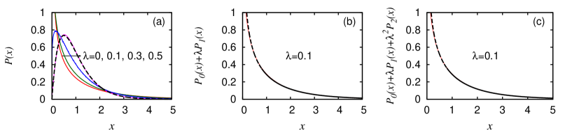
Figure 2: The steady state distribution $P(x)$ of ASCM with random sequential update: (a) obtained from Monte Carlo simulations of system size $L=1000$ for $\lambda=0,0.1,0.3,$ and $0.5$. The distribution for $\lambda=0.5$ is compared with the analytical result Eq. (36) (shown as dashed line). In (b) and (c) we have compared the distribution for $\lambda=0.1$ with the $1^{st}$ and $2^{nd}$ order perturbation results (dashed line) respectively.

There is no particular difficulty in proceeding for higher order perturbations in $\lambda,$ except that the expressions are lengthy. We have listed the $P_{k}(x)$ for $k=0,1,2$ in the Appendix.

In Fig. 2 we have compared these perturbation results with the Monte Carlo simulation of the dynamics on a one dimensional periodic system of size $L=1000.$ The steady state distribution for $\lambda=0,0.1,0.3,$ and $0.5$ are shown in Fig. 2(a). In the same figure we compare the distribution function for $\lambda=0.5$ with Eq. (36) (dashed line). The distribution for $\lambda=0.1$ (solid line) is compared with the perturbation results (dashed line) up to $1^{st}$ and $2^{nd}$ order respectively in Figs. 2(b) and (c).

4 Symmetric Sticky Chipping Model (SSCM) :

In this section we study the symmetric version of the model, namely SSCM, where $(1-\lambda)$ fraction of the mass $x_{i}$ at site $i$ is chipped off and distributed randomly among the neighbours $(i\pm 1)$; the right neighbour receives $\mu_{R}=r_{i}(1-\lambda)x_{i}$ and the left one receives the rest $\mu_{L}=(1-r_{i})(1-\lambda)x_{i}$ . Here again $r_{i}$ is a random number uniformly distributed in the interval $(0,1)$.

The criterion (14) for asymmetric mass transport models to have factorized steady state [12], does not straight forwardly extend to the symmetric case. However, to have factorized steady state for a chipping model on an arbitrary graph, it is sufficient that its chipping kernel at each site has a product form [13] similar to Eq. (14). In SSCM, this condition translates to

$$\phi_{sym}(\mu_{L},\mu_{R}|x)=\frac{u(\mu_{L})v(\mu_{R})w(x-\mu_{L}-\mu_{R})}{\int d\mu_{L}d\mu_{R}u(\mu_{L})v(\mu_{R})w(x-\mu_{L}-\mu_{R})}.$$ (43)

The chipping kernel in this model is

$$\phi_{sym}(\mu_{L},\mu_{R}|x)=\delta\left((1-\lambda)x-\mu_{L}-\mu_{R}\right)\phi(\mu_{L}|x),$$

where $\phi(\mu_{L}|x)$ is the same distribution given by Eq. (13). It is evident $\phi_{sym}(\mu_{L},\mu_{R}|x)$ can be cast into the the form (43) when $\lambda=0,$ by taking the functions $u=1=v$ (similar to ASCM) and $w=\delta(x-\mu_{L}-\mu_{R});$ thus the steady state is factorized. For $\lambda\neq 0,$ however, such product form does not exist and we proceed to calculate the steady state distribution perturbatively for both parallel and random sequential updates.

4.1 Parallel Update :

In this subsection we study the model where all the sites are updated parallely (synchronously) using the dynamics mentioned above. Explicitly,

$$x_{i}(t+1)=\lambda x_{i}(t)+(1-\lambda)[r_{i-1}x_{i-1}(t)+(1-r_{i+1})x_{i+1}(t)]$$ (44)

where, the $1^{st}$ term on the r.h.s. represents the mass that sticks to the site $i$ during the update, the $2^{nd}$ and the $3^{rd}$ term there correspond to the mass which $i^{th}$ site receives from its neighbours $i\mp 1$ respectively. Thus the steady state probability that the site $i$ has mass $x$ is given by,

$$P(x) = \int_{0}^{\infty}dx_{i-1}\int_{0}^{\infty}dx_{i}\int_{0}^{\infty}dx_{i+1}\int_{0}^{1}dr_{i-1}\int_{0}^{1}dr_{i+1}P(x_{i-1})P(x_{i})P(x_{i+1})$$ (46)

$$\delta\Big{(}x-\lambda x_{i}-(1-\lambda)[r_{i-1}x_{i-1}+(1-r_{i+1})x_{i+1}]\Big{)},$$

where we have used a mean field approximation $\langle x_{i-1}^{l}x_{i}^{m}x_{i+1}^{n}\rangle=\langle x_{i-1}^{l}\rangle\langle x_{i}^{m}\rangle\langle x_{i+1}^{n}\rangle.$ In other words three and lower order spatial correlations are ignored.

Here we intend to follow approach II. First let us express the above equation in terms of $Q(s)$, which is the Laplace transform of $P(x)$;

$$Q(s)=Q(\lambda s)V^{2}\Big{(}(1-\lambda)s\Big{)},$$ (47)

where $V(s)$ is defined by

$$V(s)=\int_{0}^{1}dr~{}Q(sr),~{}~{}~{}\mbox{or}~{}~{}~{}Q(s)=V(s)+sV^{\prime}(s).$$ (48)

In fact Eq. (47) can be written in terms of the function $V$ as

$$V(s)+sV^{\prime}(s)=\left[V(\lambda s)+\lambda sV^{\prime}(\lambda s)\right]V^{2}\Big{(}(1-\lambda)s\Big{)}.$$ (49)

Let us begin with $\lambda=0$. In this case, Eq. (49) takes the form

$$sV^{\prime}(s)-V(s)^{2}+V(s)=0,$$ (50)

where we have used $V(0)=1,$ from Eq. (2). The solution of this differential equation, with the boundary condition $V^{\prime}(0)=-1/2$ which corresponds to a fixed average mass $\langle x\rangle=1$ gives,

$$V(s)=\frac{2}{s+2},{\rm~{}and~{}thus~{}}P(x)=\mathscr{L}^{-1}\left[V(s)+sV^{\prime}(s)\right]=4xe^{-2x}.$$

This expression is identical to $P(x)$ obtained in case of ASCM with parallel update. In the following we argue that the dynamics of SSCM for $\lambda=0$ is equivalent to that of ASCM :

$$x_{i}(t+1)=r_{i-1}x_{i-1}(t)+(1-r_{i})x_{i}(t) ~{}~{}~{}~{}~{}~{}{\rm ASCM}$$

$$x_{i}(t+1)=r_{i-1}x_{i-1}(t)+(1-r_{i+1})x_{i+1}(t) ~{}~{}~{}~{}~{}~{}{\rm SSCM}.$$

Since ASCM has a product measure, the steady state remains invariant if the dynamics is changed to a mean field dynamics $x_{i}\to(r_{j}x_{j}+(1-r_{k})x_{k}),$ where for each $i,$ $j$ (and $k$) are chosen randomly from the set $\{1,2,\dots,L\}$ without replacement, $i.e.$ all the sites receive exactly two fragments, $r_{j}$ fraction of $x_{j}$ and $(1-r_{k})$ fraction of $x_{k}$. Clearly the choice $j=(i-1)$ and $k=(i+1)$ corresponds to SSCM. Thus, SSCM with $\lambda=0$ has a factorized steady state with mass distribution $P(x)$ same as ASCM.

These arguments do not extend to $\lambda\neq 0$ case, as the steady state of the corresponding asymmetric model is not factorized. We proceed with the perturbation approach. First let us expand $V$ in the Taylor series about $\lambda=0$; for any arbitrary $a,b$

$$V\Big{(}(a+b\lambda)s\Big{)}=\sum_{m=0}^{\infty}\frac{(b\lambda s)^{m}}{m!}\frac{d^{m}V(s)}{ds^{m}}\Bigg{|}_{s\to as}.$$ (51)

Each of the $V(s)$ and their derivatives are then expanded, similar to Eq. (10), as

$$V(s)=\sum_{k=0}^{\infty}\lambda^{k}V_{k}(s).$$ (52)

Now using Eqs. (51) and (52) in Eq. (49) and collecting the coefficients of different powers of $\lambda$, order by order, one can obtain a set of differential equations in terms of $V_{k}(s),$ which can be solved using the boundary conditions

$$k=0~{}~{}~{}:V_{0}(0)=1,~{}~{}~{}V_{0}^{\prime}(0)=-\frac{1}{2}$$

$$k\neq 0~{}~{}~{}:V_{k}(0)=0,~{}~{}~{}V_{k}^{\prime}(0)=0.$$ (53)

These boundary conditions on $V$ are same as Eqs. (3) and (4), which ensure that $P(x)$ is normalized and the average mass of the system is unity. Interestingly, using Eq. (12) in Eq. (48) one gets

$$V_{k}(s)=\sum_{n=0}^{\infty}(-s)^{n}A_{k}^{(n)},$$ (54)

which implies that $V_{k}(s)$ is simply the generating function of $A_{k}^{(n)}$ used in approach I.

Following the perturbation approach, we use Eqs. (51) and (52) in Eq. (49) and equate the terms which are independent of $\lambda$ and get

$$sV_{0}^{\prime}(s)-V_{0}(s)^{2}+V_{0}(s)=0,$$

which is same as Eq. (50) and we get

$$V_{0}(s)=\frac{2}{s+2},~{}~{}{\rm and}~{}~{}P_{0}(x)=4xe^{-2x}.$$

Next we move to the first order perturbation. Collecting the coefficients of $\lambda$ in Eq. (49),

$$s(s+2)^{3}V_{1}^{\prime}(s)+(s+2)^{2}(s-2)V_{1}(s)+4s^{2}=0$$

which, along with the boundary condition $V_{1}^{\prime}(0)=0$ (from Eq. (53)), results in

$$V_{1}(s)=-\frac{4s\Big{(}\ln(s+2)-\ln(2)\Big{)}}{(s+2)^{2}}.$$

Thus we obtain

$$P_{1}(x)=\mathscr{L}^{-1}\left[V_{1}(s)+sV_{1}^{\prime}(s)\right]=16e^{-2x}\left[x^{2}\Big{(}1-g(x)\Big{)}+xg(x)-\frac{1}{4}\right]$$

where $g(x)=\ln(2x)+\gamma$.

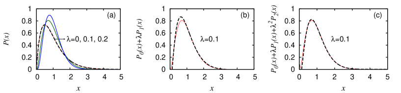
Figure 3: SSCM with parallel update : (a) $P(x)$ obtained from Monte Carlo simulations of the model on a one dimensional lattice of size $L=1000$ for $\lambda=0,0.1,$ and $0.2$. The distribution for $\lambda=0$ is compared with the exact result $P(x)=4xe^{-2x}$ (dashed line). (b) and (c) compare $P(x)$ obtained from the $1^{st}$ and $2^{nd}$ order perturbation (dashed line) respectively with the same obtained from simulations, for $\lambda=0.1$.

Following the same procedure one can obtain other higher order corrections to $P(x).$ In the Appendix, we have listed these correction terms up to $2^{nd}$ order. As described in Fig. 3, the perturbation results for $P(x)$ agree well with the actual steady state mass distribution obtained from the Monte Carlo simulation. In Fig. 3(a) we have shown the simulation results for $\lambda=0,0.1,$ and $0.2.$ In the same figure we compare the result for $\lambda=0$ with the analytically obtained result (dashed line). In Figs. 3(b) and (c) the distribution for $\lambda=0.1$ (solid line) is compared with the perturbation results (dashed line) up to $1^{st}$ and $2^{nd}$ order respectively. Clearly, as expected, the distribution matches better with the simulation results as we go to higher order.

4.2 Random sequential update :

In this subsection we study the symmetric sticky chipping model using random sequential update. At each step, a site is chosen randomly and from this site $i,$ $(1-\lambda)$ fraction of the mass $x_{i}$ is chipped off. From the chipped off mass $(1-\lambda)x_{i},$ $r_{i}$ fraction is transported to the right neighbour, and the rest goes to the left. With update of a single site, the time is increased by $\Delta t=1/L.$

The moments $\langle x_{i}^{n}\rangle$ can be expressed as

$$\langle x_{i}^{n}\rangle = \frac{1}{3}\Big{\langle}(\lambda x_{i})^{n}\Big{\rangle}+\frac{1}{3}\left\langle\Big{(}x_{i}+r_{i-1}(1-\lambda)x_{i-1}\Big{)}^{n}\right\rangle$$

$$~{}~{}~{}~{}~{}~{}~{}~{}~{}+\frac{1}{3}\left\langle\Big{(}x_{i}+(1-r_{i+1})(1-\lambda)x_{i+1}\Big{)}^{n}\right\rangle$$

$$= \frac{1}{3}\Big{\langle}(\lambda x_{i})^{n}\Big{\rangle}+\frac{2}{3}\left\langle\Big{(}x_{i}+r_{i-1}(1-\lambda)x_{i-1}\Big{)}^{n}\right\rangle.$$ (56)

The factors $\frac{1}{3}$ come from the fact that during each update, one site transports and two other sites receive the mass. Thus, probability that a site acts as a departure site is $\frac{1}{3}$ and the probability that it acts as a receiving site is $\frac{2}{3}.$

Now, consider the case $\lambda=0$. Then, Eq. (56) takes the form

$$\langle x_{i}^{n}\rangle=\frac{1}{3}\delta_{n,0}+\frac{2}{3}\langle(x_{i}+r_{i-1}x_{i-1})^{n}\rangle.$$

The additional term $\frac{1}{3}\delta_{n,0}$ appears from the fact that for $n=0,$ the first term on the r.h.s. of Eq. (56) gives $\frac{1}{3}$ for any arbitrary $\lambda$ except $\lambda=0.$

Assuming that all the two point correlations are zero in the steady state, $i.e.$ $\langle x_{i}^{m}x_{i-1}^{n}\rangle=\langle x_{i}^{m}\rangle\langle x_{i-1}^{n}\rangle,$ one can write $A^{(n)}\equiv\frac{\langle x^{n}\rangle}{(n+1)!}$ as

$$A^{(n)}=\frac{2}{n-1}\sum_{k=1}^{n-1}(n-k+1)A^{(k)}A^{(n-k)}~{}~{}~{}~{}~{}\forall~{}n\geq 2.$$ (57)

This equation can be converted to a differential equation by using $V(s)=\sum_{n=0}^{\infty}(-s)^{n}A^{(n)},$ the generating function of $A^{(n)},$

$$V^{\prime}(s)=\frac{1-3V(s)+2V^{2}(s)}{s\Big{(}3-2V(s)\Big{)}}.$$

For the usual boundary condition $V(0)=1,~{}V^{\prime}(0)=-1/2$, the solution to the above equation is

$$V(s)=\frac{2s-1+\sqrt{4s+1}}{4s}$$

which results in

$$P(x)=\mathscr{L}^{-1}\left[V(s)+sV^{\prime}(s)\right]=\frac{1}{4\sqrt{\pi x}}e^{-x/4}+\delta(x).$$ (58)

In the above expression the term $\delta(x)$ is needed to assure the normalization of $P(x)$.

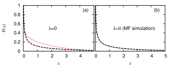
Figure 4: Comparison of Eq. (58) (dashed line) with $P(x)$ obtained from Monte Carlo simulations (solid line) of SSCM with random sequential update for $\lambda=0$ and $L=1000$. (a) The actual model. (b) The model with mean field (MF) dynamics.

In Fig. 4(a) we have compared this result with the Monte Carlo simulation of the model with $\lambda=0$. The right panel (b) shows $P(x)$ obtained from Eq. (58) along with the simulation results of the model with a mean field (MF) dynamics, i.e., $r_{i}$ and $(1-r_{i})$ fraction of the chipped off mass $(1-\lambda)x_{i}$ are transported from site $i$ to two arbitrary sites instead of being transported to the neighbours. Clearly Eq. (58) is consistent with simulation results of the MF dynamics emphasizing that Eq. (58) correctly describes the mean field distribution. On the other hand the same mass distribution obtained from Monte Carlo simulation of the actual model deviates substantially (Fig. 4(a)). This discrepancy, which originates from the mean field approximation used here (that ignores all the two point correlations), can not be healed by adding perturbative correction terms. We do not proceed further in this case.

5 Summary and conclusion :

In this article we have studied the conserved mass transport process in presence of stickiness, characterized by a parameter $\lambda$. The model in one dimension evolves using a parallel or random sequential update rule, where a fixed fraction ($i.e.~{}~{}(1-\lambda)),$ of the mass from a site is chipped off and then distributed randomly among the site and its neighbours. In the asymmetric version ASCM, the chipped off mass is distributed among the site and its right neighbour, whereas in SSCM it is distributed among both the neighbours.

For nonzero $\lambda$ the steady state distribution of these models do not have factorized form. We introduce a perturbation approach to obtain an approximate mass distribution function $P(x)=\sum_{k=0}^{\infty}\lambda^{k}P_{k}(x)$, and provide explicit form of $P_{k}(x)$ up to $2^{nd}$ order in $\lambda.$ In all cases except SSCM with random sequential update, the perturbation results agree quite well with the distribution obtained from the Monte Carlo simulation of the model, even though we have used a mean field approximation which ignores two or three point spatial correlations.

Interestingly, the steady state distribution for the following three cases, (a) ASCM with parallel update and $\lambda=0,$ (b) ASCM with random sequential update and $\lambda=\frac{1}{2},$ and (c) SSCM with parallel update and $\lambda=0,$ are identical, $P(x)=4xe^{-2x}.$ It turns out that product measure is exact only for models (a) and (c).

In absence of any general formalism, calculating the exact steady state distribution for non-equilibrium models is not always possible. The perturbation approach we discussed here is quite general and can be used in models with some small parameter to obtain steady state distribution analytically within a mean field approximation that ignores only two point correlations in all cases, except for SSCM with parallel update where both two and three point correlations are ignored.

Acknowledgements: We would like to thank the referees for their useful comments and suggestions, and U. Basu for careful reading of the manuscript.

Appendix :

The steady state distribution of the models studied here with parallel (p) and random sequential (rs) updates, using the perturbation approach, are summarized below.
Models $P(x)=P_{0}(x)+\lambda P_{1}(x)+\lambda^{2}P_{2}(x)+\dots$ ASCM (p) $P_{0}(x)=4xe^{-2x}$ $P_{1}(x)=8e^{-2x}\left[x^{2}\Big{(}1-g(x)\Big{)}+xg(x)-\frac{1}{4}\right]$ $P_{2}(x)=8e^{-2x}\Big{[}x^{3}\Big{(}g^{2}(x)-2g(x)+\frac{18-\pi^{2}}{6}\Big{)}-x^{2}\Big{(}\frac{5}{2}g^{2}(x)-2g(x)$ $~{}~{}~{}~{}~{}~{}~{}+\frac{48-5\pi^{2}}{12}\Big{)}+x\Big{(}g^{2}(x)+\frac{3}{2}g(x)-\frac{\pi^{2}}{6}\Big{)}-\frac{1}{4}\Big{(}g(x)+1\Big{)}\Big{]}+2\delta(x)$ ASCM (rs) $P_{0}(x)=\frac{1}{\sqrt{2\pi x}}e^{-x/2}$ $P_{1}(x)=\frac{1}{4\sqrt{2\pi x}}e^{-x/2}\Big{[}-x\Big{(}g(x)+2\Big{)}+g(x)+4\Big{]}+\frac{1}{2}e^{-x/2}-2\delta(x)$ $P_{2}(x)=\frac{1}{32\sqrt{2\pi x^{3}}}e^{-x/2}\Big{[}x^{3}\Big{(}g^{2}(x)+4g(x)+\frac{20-\pi^{2}}{2}\Big{)}-4x^{2}\Big{(}g^{2}(x)+6g(x)$                             $+\frac{43-3\pi^{2}}{6}\Big{)}+x\Big{(}g^{2}(x)+12g(x)-\frac{20+3\pi^{2}}{6}\Big{)}-10\Big{]}$            $-\frac{1}{8}e^{-x/2}\Big{[}x\Big{(}g(\frac{x}{4})+3\Big{)}-2g(\frac{x}{4})-10\Big{]}$ $+\frac{2}{3}\Big{[}\delta^{\prime}(x)-2\delta(x)\Big{]}$ SSCM (p) $P_{0}(x)=4xe^{-2x}$ $P_{1}(x)=16e^{-2x}\left[x^{2}\Big{(}1-g(x)\Big{)}+xg(x)-\frac{1}{4}\right]$ $P_{2}(x)=32e^{-2x}\Big{[}x^{3}\Big{(}g^{2}(x)-2g(x)+\frac{33-2\pi^{2}}{12}\Big{)}-x^{2}\Big{(}3g^{2}(x)-2g(x)$         $-H(x)+\frac{21-2\pi^{2}}{6}\Big{)}+x\Big{(}\frac{3}{2}g^{2}(x)+g(x)-H(x)-\frac{\pi^{2}}{12}\Big{)}$         $-\frac{1}{4}\Big{(}g(x)+1\Big{)}\Big{]}-8\Gamma(0,2x)(2x-1)+6\delta(x)$ SSCM (rs) $P_{0}(x)=\frac{1}{4\sqrt{\pi x}}e^{-x/4}+\delta(x)$

Here, $g(x)=\ln(2x)+\gamma,$ and $H(x)=\sum_{m=1}^{\infty}[\frac{2}{m}+\gamma+\frac{\Gamma^{\prime}(m)}{\Gamma(m)}-g(x)]\frac{(2x)^{m}}{mm!}.$
$\Gamma(0,x)$ is the incomplete gamma function and Euler constant $\gamma=0.57721...$

References :

References

- [1] Demirel Y 2007 Nonequilibrium thermodynamics: transport and rate processes in physical, chemical and biological systems Elsevier.
- [2] Privman V 2005 Nonequilibrium Statistical Mechanics in One Dimension Cambridge University Press; Exactly solvable models for many-body systems far from equilibrium, Phase Transitions and Critical Phenomena (Ed. by C. Domb and J. L. Lebowitz) Vol. 19.
- [3] Majumdar S N, Krishnamurthy S, and Barma M 1998 Phys. Rev. Lett. 81 3691; Yamamoto H and Ohtsuki T 2010 Phys. Rev. E 81 061116; Kwon S, Lee S, and Kim Y 2006 Phys. Rev. E 73 056102; Jain K, Barma M 2001 Phys. Rev. E 64 016107; Rajesh R and Majumdar S N 2001 Phys. Rev. E 63 036114.
- [4] Evans M R, Hanney T 2005 J. Phys. A: Math. Gen. 38 19.
- [5] White W H 1982 J. Colloid Interface Sci. 87 204.
- [6] Ziff R M 1980 J. Stat. Phys. 23 241; Krapivsky P L, Redner S, 1996 Phys. Rev. E 54 3553.
- [7] Scheidegger A E 1967 Bull. I.A.S.H. 12 15.
- [8] Derrida B, Evans M R, Hakim V, and Pasquier V 1993 J. Phys. A : Math. Gen. 26 1493.
- [9] Ispolatov S, Krapivsky P L, and Redner S 1998 Eur. Phys. J. B2 267.
- [10] Rajesh R and Majumdar S N 2000 J. Stat. Phys. 99 943.
- [11] Majumdar S N, Evans M R, and Zia R K P 2005 Phys. Rev. Lett. 94 180601.
- [12] Evans M R, Majumdar S N, and Zia R K P 2004 J. Phys. A: Math. Gen. 37 L275.
- [13] Evans M R, Majumdar S N, and Zia R K P 2006 J. Phys. A: Math. Gen. 39 4859.