Controllable entanglement preparations between atoms in spatially-separated cavities via quantum Zeno dynamics

Abstract

By using quantum Zeno dynamics, we propose a controllable approach to deterministically generate tripartite GHZ states for three atoms trapped in spatially separated cavities. The nearest-neighbored cavities are connected via optical fibers and the atoms trapped in two ends are tunably driven. The generation of the GHZ state can be implemented by only one step manipulation, and the EPR entanglement between the atoms in two ends can be further realized deterministically by Von Neumann measurement on the middle atom. Note that the duration of the quantum Zeno dynamics is controllable by switching on/off the applied external classical drivings and the desirable tripartite GHZ state will no longer evolve once it is generated. The robustness of the proposal is numerically demonstrated by considering various decoherence factors, including atomic spontaneous emissions, cavity decays and fiber photon leakages, etc. Our proposal can be directly generalized to generate multipartite entanglement by still driving the atoms in two ends.

I introduction

Quantum entanglement, as a fundamental aspect in quantum mechanics, has occupied a central place in modern research because of its promise of enormous utility in quantum computing 1 ; 2 ; 3 , cryptography 2 ; 4 , etc. Generally speaking, the more particles that can be entangled, the more clearly nonclassical effects are exhibited and the more useful the states are for quantum applications. Typically, tripartite GHZ state, first proposed by Greenberger, Horne, and Zeilinger, provides a possibility to test quantum mechanics against local hidden theory without inequality ghz and has practical applications in e.g., quantum secrete sharing hbb .

Recently, many theoretical schemes ghz_t1 ; ghz_t2 ; ghz_t3 ; ghz_t4 have been proposed to generate multipartite GHZ states, and a series of experimental preparations ghz_e1 ; ghz_e2 ; ghz_e3 have already been realized. The physical systems utilized to these generations include superconducting circuits ghz_t4 ; ghz_e3 , trapped ions ghz_e2 , and cavity QED systems, etc.. It is well-known that cavity QED, where atoms interact with quantized electromagnetic fields inside a cavity, is a useful platform to demonstrate fundamental quantum mechanics laws and for the implementation of quantum information processing qed . Specifically, numerous proposals with cavity QED have been made for entangling atoms either inside a cavity cz ; hl or trapped individually in different cavities czkm ; ecz ; bkpv ; lssh ; pk . For example, Pellizzari p proposed an approach to realize the reliable transfer of quantum information between two atoms in distant cavities connected by an optical fiber. Based on this proposal, various schemes 19 ; 20 ; 21 ; 22 ; 23 ; 24 ; 25 ; 26 ; 27 ; zl have been proposed to realize the quantum manipulations of the atoms trapped in different cavities connected via optical fibers. However, these models either require strong cavity-fiber coupling 24 (which is not easy to achieve in the usual experiment), or need many laser beams to implement the desirable manipulations 25 (this increases the experimental complication), or is sensitive to the decays of cavity fields and fiber modes zl (which limits its scalability).

Here, by using quantum Zeno dynamics we propose an alternative approach to entangle the atoms trapped in the distant cavities connected by optical fibers. It is well-known that quantum Zeno effect is an interesting phenomenon in quantum mechanics. Due to this effect the quantum system remains in its initial state via frequently measurements. Facchi et al zeno1 ; zeno2 ; zeno3 showed that this effect does not necessarily freeze the dynamics. Instead, by frequently projecting onto a multidimensional subspace, the system could evolve away from its initial state, although it remains in the so-called “Zeno subspace” zeno1 ; zeno4 . Moreover, without making use of projection operators and nonunitary dynamics, the quantum Zeno effect can also be expressed in terms of a continuous coupling between the system and detector zeno3 . Generally, the system and its continuously coupling detector can be governed by the total Hamiltonian $H_{K}=H+KH_{a}$, with $H$ is for the quantum system investigated and the $H_{a}$ describing the additional interaction with the detector, and $K$ the coupling constant. In the limit $K\rightarrow\infty$, the subsystem of interest is dominated by the evolution operator $U(t)=\lim_{K\rightarrow\infty}\exp(iKH_{a}t)U_{K}(t)$ which takes the form $U(t)=\exp(-it\sum_{n}P_{n}HP_{n})$ zeno3 . Here, $P_{n}$ is the eigenprojection of $H_{a}=\sum_{n}\lambda_{n}P_{n}$ corresponding to the eigenvalue $\lambda_{n}$. As a consequence, the system-detector can be described by the evolution operator $U_{K}(t)\sim\exp(-iKH_{a}t)U(t)=\exp[-i\sum_{n}(K\lambda_{n}P_{n}+P_{n}HP_{n})t]$. This result is of great importance in view of practical applications of the quantum Zeno dynamics, such as to prepare various quantum states state1 ; state2 ; me and to implement the quantum gates gate1 ; gate2 ; gate3 ; gate4 .

Compared with previous protocols 24 ; 25 ; zl for generating GHZ states by selective absorption and emission of photons, adiabatic passages, and dispersive interactions between the atoms and cavities, etc., our approach possesses the following advantages: (i) the expected entanglement can be established by only one step operation, (ii) it is robust with respect to parameter imprecision and atomic and fibers’ dissipations, (iii) under the Zeno condition, the cavity fields are not excited really and thus is insensitive to the decays of the cavities, (iv) the generalization to N-atom entanglement is direct, and no matter how many atoms are involved, two laser beams are enough to implement the generations.

The paper is organized as follows. In section II, we present our generic approach by using quantum Zeno dynamics to implement the GHZ entanglement of the atoms trapped in three fiber-connected cavities. The validity of the used quantum Zeno dynamics is analyzed by numerical method in detail. The direct generalization for entangling the $N$ atoms trapped individually in $N$ cavity is provided in Sec. III. Finally, in Sec. IV we discuss the feasibility of our proposal and give our conclusions.

II Generation of GHZ state of atoms trapped in different cavities by quantum Zeno dynamics

We consider the physical configuration shown in the Fig. 1, three $\Lambda$-type atoms are trapped in three distant optical cavities coupled by two short optical fibers. Each atom has one excited state $|e\rangle$ and two dipole-transition forbidden ground states $|0\rangle$, $|1\rangle$. The first and third atomic transitions $|1\rangle\leftrightarrow|e\rangle$ are driven resonantly by classical lasers with the couplings coefficient $\Omega_{1}$ and $\Omega_{3}$, respectively. The other atomic transition is resonantly coupled to the corresponding cavity mode with coupling constant $g_{i,r(l)}$ ($i=1,2,3$). The subscript $r(l)$ denotes the right (left) circularly polarization. In the short fiber limit, $(2L\bar{v})/(2\pi c)\ll 1$, where $L$ is the length of the fiber and $\bar{v}$ is the decay rate of the cavity fields into a continuum of fiber modes 19 . In the interaction picture, the Hamiltonian of the whole system can be written as

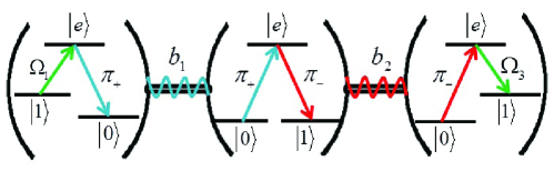
Figure 1: Zeno manipulations of atoms in spatially-separated cavities connected via optical fibers. Here, $\Omega_{1}$ ($\Omega_{3}$) is the classical field coupled to the first (third) atom, and $b_{1}$ and $b_{2}$ are the bosonic operators in fibers and couple to the corresponding cavity modes.

$$H_{\mathrm{total}}=H_{l}+H_{a-c-f},$$ (1)

$$H_{l}=\Omega_{1}|e\rangle_{1}\langle 1|+\Omega_{3}|e\rangle_{3}\langle 1|+\mathrm{h.c.},$$ (2)

$$H_{a-c-f} = g_{1,r}a_{1,r}|e\rangle_{1}\langle 0|+g_{2,r}a_{2,r}|e\rangle_{2}\langle 0|+g_{2,l}a_{2,l}|e\rangle_{2}\langle 1|+g_{3,l}a_{3,l}|e\rangle_{3}\langle 0|$$ (3)

$$+ v_{1}b_{1}^{\dagger}(a_{1,r}+a_{2,r})+v_{2}b_{2}^{\dagger}(a_{2,l}+a_{3,l})+\mathrm{h.c.},$$

where $a$ and $b$ are the annihilation operators associated with the modes of cavity and fiber respectively and $v_{i}$($i=1,2$) is the corresponding cavity-fiber coupling constant. We assume that $g_{1,r}=g_{2,r(l)}=g_{3,l}=g$ and $v_{1}=v_{2}=v$ for convenience. If the initial state of the whole system is $|1,0,0\rangle_{a}|0\rangle_{c_{1}}|0\rangle_{f_{1}}|0,0\rangle_{c_{2}}|0\rangle_{f_{2}}|0\rangle_{c_{3}}$, then the evolution of system will be restricted in the subspace spanned by

$$|\phi_{1}\rangle = |1,0,0\rangle_{a}|0\rangle_{c_{1}}|0\rangle_{f_{1}}|0,0\rangle_{c_{2}}|0\rangle_{f_{2}}|0\rangle_{c_{3}},\quad|\phi_{2}\rangle=|e,0,0\rangle_{a}|0\rangle_{c_{1}}|0\rangle_{f_{1}}|0,0\rangle_{c_{2}}|0\rangle_{f_{2}}|0\rangle_{c_{3}},$$

$$|\phi_{3}\rangle = |0,0,0\rangle_{a}|1\rangle_{c_{1}}|0\rangle_{f_{1}}|0,0\rangle_{c_{2}}|0\rangle_{f_{2}}|0\rangle_{c_{3}},\quad|\phi_{4}\rangle=|0,0,0\rangle_{a}|0\rangle_{c_{1}}|1\rangle_{f_{1}}|0,0\rangle_{c_{2}}|0\rangle_{f_{2}}|0\rangle_{c_{3}},$$

$$|\phi_{5}\rangle = |0,0,0\rangle_{a}|0\rangle_{c_{1}}|0\rangle_{f_{1}}|1,0\rangle_{c_{2}}|0\rangle_{f_{2}}|0\rangle_{c_{3}},\quad|\phi_{6}\rangle=|0,e,0\rangle_{a}|0\rangle_{c_{1}}|0\rangle_{f_{1}}|0,0\rangle_{c_{2}}|0\rangle_{f_{2}}|0\rangle_{c_{3}},$$

$$|\phi_{7}\rangle = |0,1,0\rangle_{a}|0\rangle_{c_{1}}|0\rangle_{f_{1}}|0,1\rangle_{c_{2}}|0\rangle_{f_{2}}|0\rangle_{c_{3}},\quad|\phi_{8}\rangle=|0,1,0\rangle_{a}|0\rangle_{c_{1}}|0\rangle_{f_{1}}|0,0\rangle_{c_{2}}|1\rangle_{f_{2}}|0\rangle_{c_{3}},$$

$$|\phi_{9}\rangle = |0,1,0\rangle_{a}|0\rangle_{c_{1}}|0\rangle_{f_{1}}|0,0\rangle_{c_{2}}|0\rangle_{f_{2}}|1\rangle_{c_{3}},\quad|\phi_{10}\rangle=|0,1,e\rangle_{a}|0\rangle_{c_{1}}|0\rangle_{f_{1}}|0,0\rangle_{c_{2}}|0\rangle_{f_{2}}|0\rangle_{c_{3}},$$

$$|\phi_{11}\rangle = |0,1,1\rangle_{a}|0\rangle_{c_{1}}|0\rangle_{f_{1}}|0,0\rangle_{c_{2}}|0\rangle_{f_{2}}|0\rangle_{c_{3}},$$ (4)

where $|i,j,k\rangle_{a}$ ($i,j,k=0,1,e$) denotes the state of atoms in each cavity, $n$ in $|n\rangle_{s}$ ($s=c_{1},f_{1},c_{2},f_{2},c_{3}$) denotes the photon number in cavities or fibers.

Under the Zeno condition $g,v\gg\Omega_{1},\Omega_{3}$, the above Hilbert subspace is split into nine invariant Zeno subspaces zeno3

$$\Gamma_{P_{1}} = \{|\phi_{1}\rangle,|\psi_{1}\rangle,|\phi_{11}\rangle\},\quad\Gamma_{P_{2}}=\{|\psi_{2}\rangle\},$$

$$\Gamma_{P_{3}} = \{|\psi_{3}\rangle\},\quad\Gamma_{P_{4}}=\{|\psi_{4}\rangle\},\quad\Gamma_{P_{5}}=\{|\psi_{5}\rangle\},\quad\Gamma_{P_{6}}=\{|\psi_{6}\rangle\},$$ (5)

$$\Gamma_{P_{7}} = \{|\psi_{7}\rangle\},\quad\Gamma_{P_{8}}=\{|\psi_{8}\rangle\},\quad\Gamma_{P_{9}}=\{|\psi_{9}\rangle\}$$

corresponding to the projections

$$P_{i}^{\alpha}=|\alpha\rangle\langle\alpha|,\quad(|\alpha\rangle\in\Gamma_{P_{i}})$$ (6)

with eigenvalues $\lambda_{1}=0$, $\lambda_{2}=-\sqrt{(g^{2}+2v^{2}-A)/2}$, $\lambda_{3}=\sqrt{(g^{2}+2v^{2}-A)/2}$, $\lambda_{4}=-\sqrt{(3g^{2}+2v^{2}-A)/2}$, $\lambda_{5}=\sqrt{(3g^{2}+2v^{2}-A)/2}$, $\lambda_{6}=-\sqrt{(3g^{2}+2v^{2}+A)/2}$, $\lambda_{7}=\sqrt{(3g^{2}+2v^{2}+A)/2}$, $\lambda_{8}=-\sqrt{(g^{2}+2v^{2}+A)/2}$, $\lambda_{9}=\sqrt{(g^{2}+2v^{2}+A)/2}$, where $A=\sqrt{g^{4}+4v^{4}}$. Here,

$$|\psi_{1}\rangle = N_{1}\left(|\phi_{2}\rangle-\frac{g}{v}|\phi_{4}\rangle+|\phi_{6}\rangle-\frac{g}{v}|\phi_{8}\rangle+|\phi_{10}\rangle\right)$$

$$|\psi_{2}\rangle = N_{2}\left(-|\phi_{2}\rangle+\epsilon_{1}|\phi_{3}\rangle-\eta_{1}|\phi_{4}\rangle-\chi_{1}|\phi_{5}\rangle+\chi_{1}|\phi_{7}\rangle+\eta_{1}|\phi_{8}\rangle-\epsilon_{1}|\phi_{9}\rangle+|\phi_{10}\rangle\right)$$

$$|\psi_{3}\rangle = N_{3}\left(-|\phi_{2}\rangle-\epsilon_{1}|\phi_{3}\rangle-\eta_{1}|\phi_{4}\rangle+\chi_{1}|\phi_{5}\rangle-\chi_{1}|\phi_{7}\rangle+\eta_{1}|\phi_{8}\rangle+\epsilon_{1}|\phi_{9}\rangle+|\phi_{10}\rangle\right)$$

$$|\psi_{4}\rangle = N_{4}\left(|\phi_{2}\rangle-\mu_{1}|\phi_{3}\rangle-\zeta_{1}|\phi_{4}\rangle+\delta_{1}|\phi_{5}\rangle-\theta_{1}|\phi_{6}\rangle+\delta_{1}|\phi_{7}\rangle-\zeta_{1}|\phi_{8}\rangle-\mu_{1}|\phi_{9}\rangle+|\phi_{10}\rangle\right)$$

$$|\psi_{5}\rangle = N_{5}\left(|\phi_{2}\rangle+\mu_{1}|\phi_{3}\rangle-\zeta_{1}|\phi_{4}\rangle-\delta_{1}|\phi_{5}\rangle-\theta_{1}|\phi_{6}\rangle-\delta_{1}|\phi_{7}\rangle-\zeta_{1}|\phi_{8}\rangle+\mu_{1}|\phi_{9}\rangle+|\phi_{10}\rangle\right)$$ (7)

$$|\psi_{6}\rangle = N_{6}\left(-|\phi_{2}\rangle+\epsilon_{2}|\phi_{3}\rangle-\eta_{2}|\phi_{4}\rangle+\chi_{2}|\phi_{5}\rangle-\chi_{2}|\phi_{7}\rangle+\eta_{2}|\phi_{8}\rangle-\epsilon_{2}|\phi_{9}\rangle+|\phi_{10}\rangle\right)$$

$$|\psi_{7}\rangle = N_{7}\left(-|\phi_{2}\rangle-\epsilon_{2}|\phi_{3}\rangle-\eta_{2}|\phi_{4}\rangle-\chi_{2}|\phi_{5}\rangle+\chi_{2}|\phi_{7}\rangle+\eta_{2}|\phi_{8}\rangle+\epsilon_{2}|\phi_{9}\rangle+|\phi_{10}\rangle\right)$$

$$|\psi_{8}\rangle = N_{8}\left(|\phi_{2}\rangle-\mu_{2}|\phi_{3}\rangle+\zeta_{2}|\phi_{4}\rangle-\delta_{2}|\phi_{5}\rangle+\theta_{2}|\phi_{6}\rangle-\delta_{2}|\phi_{7}\rangle+\zeta_{2}|\phi_{8}\rangle-\mu_{2}|\phi_{9}\rangle+|\phi_{10}\rangle\right)$$

$$|\psi_{9}\rangle = N_{9}\left(|\phi_{2}\rangle+\mu_{2}|\phi_{3}\rangle+\zeta_{2}|\phi_{4}\rangle+\delta_{2}|\phi_{5}\rangle+\theta_{2}|\phi_{6}\rangle+\delta_{2}|\phi_{7}\rangle+\zeta_{2}|\phi_{8}\rangle+\mu_{2}|\phi_{9}\rangle+|\phi_{10}\rangle\right)$$

with

$$\epsilon_{1} = \frac{\sqrt{g^{2}+2v^{2}-A}}{\sqrt{2}g},\quad\eta_{1}=\frac{-g^{2}+2v^{2}-A}{2gv},\quad\chi_{1}=\frac{\sqrt{g^{2}+2v^{2}-A}(g^{2}+A)}{2\sqrt{2}gv^{2}},$$

$$\mu_{1} = \frac{\sqrt{3g^{2}+2v^{2}-A}}{\sqrt{2}g},\quad\zeta_{1}=\frac{-g^{2}-2v^{2}+A}{2gv},\quad\delta_{1}=\frac{\sqrt{3g^{2}+2v^{2}-A}(-g^{2}+A)}{2\sqrt{2}gv^{2}},\quad\theta_{1}=\frac{-g^{2}+A}{v^{2}},$$

$$\epsilon_{2} = \frac{\sqrt{g^{2}+2v^{2}+A}}{\sqrt{2}g},\quad\eta_{2}=\frac{-g^{2}+2v^{2}+A}{2gv},\quad\chi_{2}=\frac{\sqrt{g^{2}+2v^{2}+A}(-g^{2}+A)}{2\sqrt{2}gv^{2}},$$

$$\mu_{2} = \frac{\sqrt{3g^{2}+2v^{2}+A}}{\sqrt{2}g},\quad\zeta_{2}=\frac{g^{2}+2v^{2}+A}{2gv},\quad\delta_{2}=\frac{\sqrt{3g^{2}+2v^{2}+A}(g^{2}+A)}{2\sqrt{2}gv^{2}},\quad\theta_{2}=\frac{g^{2}+A}{v^{2}},$$ (8)

and $N_{i}$ ($i=1,2,3,...,9$) being the normalization factor for the eigenstate $|\psi_{i}\rangle$. Under above condition, the system can be effectively described by the following Hamiltonian

$$H_{\mathrm{total}} \simeq \sum_{i,\alpha,\beta}\lambda_{i}P_{i}^{\alpha}+P_{i}^{\alpha}H_{l}P_{i}^{\beta}$$ (9)

$$= \sum_{i=2}^{9}\lambda_{i}|\psi_{i}\rangle\langle\psi_{i}|+N_{1}(\Omega_{1}|\phi_{1}\rangle\langle\psi_{1}|+\Omega_{3}|\phi_{11}\rangle\langle\psi_{1}|+\mathrm{h.c.})$$

It reduces to

$$H_{\mathrm{eff}}=N_{1}(\Omega_{1}|\phi_{1}\rangle\langle\psi_{1}|+\Omega_{3}|\phi_{11}\rangle\langle\psi_{1}|+\mathrm{h.c.}),$$ (10)

if the initial state is $|\phi_{1}\rangle$. The effective Hamiltonian $H_{\mathrm{eff}}$ implies that the evolution of system is restricted in the subspace, wherein the cavity modes are kept in the vacuum. Consequently, after the evolution time $t$ the state of the system becomes

$$|\Psi(t)\rangle = \frac{\cos(N_{1}t\sqrt{\Omega_{1}^{2}+\Omega_{3}^{2}})\Omega_{1}^{2}+\Omega_{3}^{2}}{\Omega_{1}^{2}+\Omega_{3}^{2}}|\phi_{1}\rangle-\frac{i\Omega_{1}\sqrt{\Omega_{1}^{2}+\Omega_{3}^{2}}\sin(N_{1}t\sqrt{\Omega_{1}^{2}+\Omega_{3}^{2}})}{\Omega_{1}^{2}+\Omega_{3}^{2}}|\psi_{1}\rangle$$ (11)

$$+ \frac{[\cos(N_{1}t\sqrt{\Omega_{1}^{2}+\Omega_{3}^{2}})-1]\Omega_{1}\Omega_{3}}{\Omega_{1}^{2}+\Omega_{3}^{2}}|\phi_{11}\rangle.$$

Obviously, if $\Omega_{1}=(\sqrt{2}+1)\Omega_{3}$ and the evolution time is set as $t=\tau=\pi/N_{1}\sqrt{\Omega_{1}^{2}+\Omega_{3}^{2}}$, then the triatomic GHZ state $|\Psi\rangle_{a}$ can be generated, i.e.,

$$|\Psi(\tau)\rangle=-\frac{1}{\sqrt{2}}(|\phi_{1}\rangle+|\phi_{11}\rangle)=|\Psi\rangle_{a}\otimes|0\rangle_{c_{1}}|0\rangle_{f_{1}}|0,0\rangle_{c_{2}}|0\rangle_{f_{2}}|0\rangle_{c_{3}},\,\,|\Psi\rangle_{a}=-\frac{1}{\sqrt{2}}(|1,0,0\rangle_{a}+|0,1,1\rangle_{a}).$$ (12)

It is emphasized that the duration $\tau$ depends directly on the Rabi frequencies $\Omega_{1}$ and $\Omega_{3}$ applied simultaneously. Thus, the above quantum Zeno dynamics stops once the classical fields $\Omega_{1}$ and $\Omega_{3}$ are switched off simultaneously. Fortunately, one can easily check that $H_{a-c-f}|\Psi(\tau)\rangle=0$, which means that generated GHZ state does not evolve when the controllable quantum Zeno dynamics vanishes.

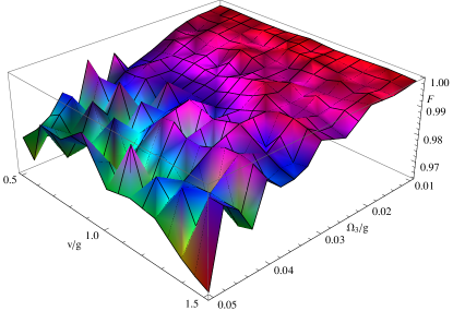
Figure 2: The influence of the ratios: $\Omega_{3}/g$ and $v/g$, on the fidelity of the prepared GHZ state.

Furthermore, if we perform a single-qubit rotation $R_{x}(\pi/4)(=\exp(i\sigma_{x}\cdot\pi/4))$ on the middle atom, then the tripartite GHZ state reduces to the state: $[(|1,0\rangle_{1,3}+i|0,1\rangle_{1,3})|0\rangle_{2}+(i|1,0\rangle_{1,3}+|0,1\rangle_{1,3})|1\rangle_{2}]/2$. Consequently, the EPR entanglement between two distant atoms can be deterministically obtained by projective measurement on the middle atom (no matter it is found at which state) wei-prb-2005 , without taking any operation on the first and third atom directly.

It is clear that the validity of our scheme mainly relies on if the so-called Zeno condition $g,v\gg\Omega_{1},\Omega_{3}$ is satisfied robustly. Now, we discuss how the ratio $\Omega_{3}/g$ influences the fidelity $F=|\langle\Psi(\tau)|\varphi(\tau)\rangle|^{2}$, with $|\varphi(\tau)\rangle$ being the relevant final state evolved by the original $H_{\mathrm{total}}$ defined in Eq.(1). On the other hand, the ratio $v/g$ is another important factor affecting the fidelity 19 ; 20 ; 21 ; 24 . Indeed, from Fig. 2 we see that the smaller the ratio $\Omega_{3}/g$ corresponds to the higher fidelity. We also note that, even at the relatively-low ratio $v/g=0.5$, the fidelity is still high, i.e., above 97%. This is very important for the practical application of our scheme, as the large cavity-fiber coupling is not easy to be satisfied in the realistic experiments. Furthermore, in order to obtain high fidelity in moderate time, we can choose typically the ratios: $\Omega_{3}/g=0.04$ and $v/g=1$.

Our proposal is also robust for the imprecision of experimental parameters. Indeed, our previous discussions are based on certain ideal assumptions, e.g., $g_{i,r(l)}\equiv g$, $v_{i}\equiv v$. Practically, the coupling strengths $g_{i,r(l)}$ depend on the positions of the atoms in the cavities, and thus certain deviations are unavoidable. To numerically consider these deviations, we typically set $g_{2,r(l)}=g$, $g_{1,r}=g+\delta g_{1}$ and $g_{3,l}=g+\delta g_{3}$ for simulations. In Fig. 3(a), the fidelity of the prepared state versus the variation $\delta g_{1}$ and $\delta g_{3}$ is plotted.

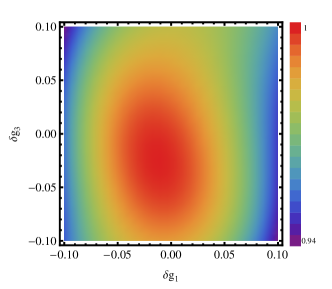
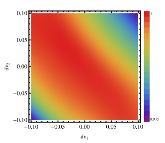
Figure 3: The fidelity of the three-atom GHZ state versus various parameter errors: (a) $\delta g_{1}$ and $\delta g_{3}$; (b) $\delta v_{1}$ and $\delta v_{2}$.

It is seen that, even under a deviation $|\delta g_{1,3}|=10\%g$, the fidelity is still sufficiently high, e.g., larger than 94%. Similarly, we plot the fidelity versus the deviation of the cavity-fiber coupling ($v$) in Fig. 3(b), and find also that the great robustness against the errors in the selected parameters.

We now numerically verify that the above effective dynamics restricted in the subspace without exciting the cavity modes is also robust. In fact, considering all possible states of the system, the state at the time $t$ reads $|\varphi_{total}\rangle=\sum_{i}c_{i}(t)|\phi_{i}\rangle$ within the subspace spanned by the basic state vectors in Eq. (II). The occupation probability for each state vector $|\phi_{i}\rangle$ during the evolution is $P_{i}(t)=|c_{i}(t)|^{2}$, and satisfies the condition $\sum_{i}P_{i}(t)=1$. By solving the Schrödinger equation, the variation of the occupation probability $P_{c}(t)$ ($\equiv\sum_{i=3,5,7,9}P_{i}(t)$) is portrayed in Fig. 4 (red line).

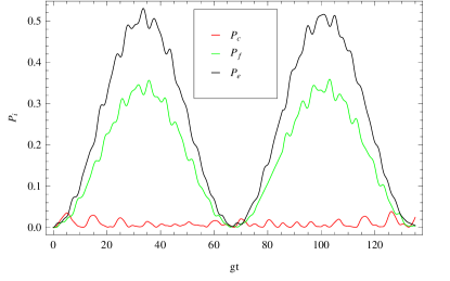
Figure 4: The population probabilities of cavity photonic state $P_{c}$, fiber photonic state $P_{f}$ and the atomic excited state $P_{e}$ versus the dimensionless parameter $gt$ by exactly solving the evolution equation of the system without any approximation.

As shown in Fig. 4, the occupation probability of the cavity photonic state is less than $0.04$. Therefore, our claim that the scheme is immune to the cavity decay seems justifiable. Meanwhile, Fig. 4 also describes the occupation probabilities $P_{f}(t)$($\equiv\sum_{i=4,8}P_{i}(t)$, green line) and $P_{e}(t)$($\equiv\sum_{i=2,6,10}P_{i}(t)$, black line) for those states, wherein the photon is in the fiber and one of the atoms in its excited state, respectively. Since $P_{e}>P_{f}$ in Fig. 4, our protocol is more sensitive to atomic spontaneous emission than the fiber loss. To check this, let us investigate the evolution of the system governed by the following non-Hermitian Hamiltonian

$$H_{\mathrm{dec}}=H_{\mathrm{total}}-\frac{i\gamma}{2}\sum_{i=1}^{3}|e\rangle_{i}\langle e|-\frac{i\kappa_{c}}{2}\left(\sum_{i=1,2}a^{\dagger}_{i,r}a_{i,r}+\sum_{i=2,3}a^{\dagger}_{i,l}a_{i,l}\right)-\frac{i\kappa_{f}}{2}\sum_{j=1,2}b_{i}^{\dagger}b_{i},$$ (13)

where $\gamma$ is the spontaneous emission rate for atoms and $\kappa_{c(f)}$ denotes the decay rate of the cavity modes (fiber modes).

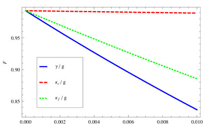
Figure 5: The influences of atomic spontaneous emission $\gamma/g$, cavity field decay $\kappa_{c}/g$ and fiber photonic leakage $\kappa_{f}/g$ on the fidelity of the triatomic GHZ state for the typical ratios: $\Omega_{3}/g=0.04$ and $v/g=1$.

It is seen from Fig. 5 that the atomic spontaneous emission is the dominant factor of degrading the fidelity of the generated GHZ state. This can also be seen directly in the explicit form of the state $|\psi_{1}\rangle$, where the population probability of the atomic excited state is larger than that of the photon in fiber.

III Generalization to N-atom entanglement

We now generalize the present scheme to generate $N$-atom GHZ states. Let us consider the configuration shown in Fig. 6, where $N$ atoms are individually trapped in $N$ cavities connected by $N-1$ short fibers. The level configuration of the atoms between two ends are chosen the same as that of the middle atom in the above 3-atom case. The Hamiltonian of the present system reads

$$H^{\prime}_{total}=H^{\prime}_{l}+H^{\prime}_{\mathrm{a-c-f}}$$ (14)

where

$$H^{\prime}_{l}=\Omega_{1}|e\rangle_{1}\langle 1|+\Omega_{N}|e\rangle_{N}\langle 1|+\mathrm{h.c.}$$ (15)

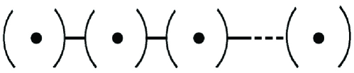
Figure 6: $N$ atom trapped in distant cavities.

$$H^{\prime}_{\mathrm{a-c-f}} = g_{1}a_{1,r}|e\rangle_{1}\langle 0|+\sum_{j=1}^{k}(g_{2j,r}a_{2j,r}|e\rangle_{2j}\langle 0|+g_{2j,l}a_{2j,l}|e\rangle_{2j}\langle 1|)$$ (16)

$$+ \sum_{j=1}^{k-1}(g_{2j+1,r}a_{2j+1,r}|e\rangle_{2j+1}\langle 1|+g_{2j+1,l}a_{2j+1,l}|e\rangle_{2j+1}\langle 0|)+g_{N}a_{N,l}|e\rangle_{1}\langle 0|$$

$$+ \sum_{j=1}^{k}[v_{2j-1}b_{2j-1}^{+}(a_{2j-1,r}+a_{2j,r})+v_{2j}b_{2j}^{+}(a_{2j,l}+a_{2j+1,l})]+\mathrm{h.c.}.$$

Without loss of generality, we consider the case where $N$ is odd number ($N=2k+1,\,k=1,2,3,...$), and $g_{i,r(l)}=g$, $v_{i}=v$. If the initial state of the whole system is prepared at the state $|1,0,0,...,0\rangle_{a}|0\rangle_{all}$, then the system will evolve within the subspace $\Gamma_{\mathrm{full}}$ spanned by the vectors: $\{|\phi^{\prime}_{1}\rangle,|\phi^{\prime}_{2}\rangle,|\phi^{\prime}_{3}\rangle,...,|\phi^{\prime}_{8k+3}\rangle\}$:

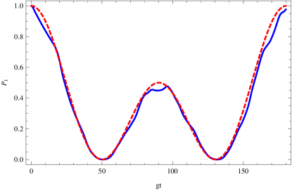
Figure 7: (Color online) The occupation probabilities of the state $|\phi^{\prime}_{1}\rangle$ versus the dimensionless parameter $gt$ under the total Hamiltonian (solid-line) and effective Hamiltonian (dotted-line).

$$|\phi^{\prime}_{1}\rangle = |1,0,0,...,0\rangle_{a}|0\rangle_{all},\quad|\phi^{\prime}_{2}\rangle=|e,0,0,...,0\rangle_{a}|0\rangle_{all},\quad|\phi^{\prime}_{3}\rangle=|0,0,0,...,0\rangle_{a}|1\rangle_{c_{1}},$$

$$|\phi^{\prime}_{4}\rangle = |0,0,0,...,0\rangle_{a}|1\rangle_{f_{1}},\quad|\phi^{\prime}_{5}\rangle=|0,0,0,...,0\rangle_{a}|1,0\rangle_{c_{2}},\quad|\phi^{\prime}_{6}\rangle=|0,e,0,...,0\rangle_{a}|0\rangle_{all},$$

$$|\phi^{\prime}_{7}\rangle = |0,1,0,...,0\rangle_{a}|0,1\rangle_{c_{2}},\quad|\phi^{\prime}_{8}\rangle=|0,1,0,...,0\rangle_{a}|1\rangle_{f_{2}},\quad|\phi^{\prime}_{9}\rangle=|0,1,0,...,0\rangle_{a}|0,1\rangle_{c_{3}},$$ (17)

$$|\phi^{\prime}_{10}\rangle = |0,1,e,...,0\rangle_{a}|0\rangle_{all},\quad...\quad|\phi^{\prime}_{8k+3}\rangle=|0,1,1,...,1\rangle_{a}|0\rangle_{all}$$

where $|0\rangle_{all}$ means that all boson modes are in the vacuum state, $n$ ($n_{1}$, $n_{2}$) in $|n\rangle_{s}$ or $|n_{1},n_{2}\rangle_{s}$ ($s=c_{i},f_{i}$) denotes the photon number in the corresponding resonator while other cavities or fibers are in the vacuum state. Similar to the above procedure, we get the effective Hamiltonian

$$H^{\prime}_{\mathrm{eff}}=N^{\prime}_{1}(\Omega_{1}|\phi^{\prime}_{1}\rangle\langle\psi^{\prime}_{1}|+\Omega_{N}|\phi^{\prime}_{8k+3}\rangle\langle\psi^{\prime}_{1}|+\mathrm{h.c.}),$$ (18)

where

$$|\psi^{\prime}_{1}\rangle=N^{\prime}_{1}\left(\sum_{i=1}^{N}|\phi^{\prime}_{4i-2}\rangle-\sum_{i=1}^{N-1}\frac{g}{v}|\phi^{\prime}_{4i}\rangle\right).$$ (19)

Set $\Omega_{1}=(\sqrt{2}+1)\Omega_{N}$ and the interaction time $\tau^{\prime}=\pi/N_{1}^{\prime}\sqrt{\Omega_{1}^{2}+\Omega_{N}^{2}}$, the desirable $N$-atomic GHZ state

$$|\Psi(\tau^{\prime})\rangle=-\frac{1}{\sqrt{2}}(|\phi^{\prime}_{1}\rangle+|\phi^{\prime}_{8k+3}\rangle)=-\frac{1}{\sqrt{2}}(|1,0,0,...,0\rangle_{a}+|0,1,1,...,1\rangle_{a})\otimes|0\rangle_{all}$$ (20)

can be generated. In order to test the effectiveness of our proposal, we consider specifically, for example, the case of five atoms. In Fig. 7, we plot the time-evolution behaviors of the occupation probability in the initial state $|\phi^{\prime}_{1}\rangle$ governed by total Hamiltonian (Eq. (14)) and by the effective Hamiltonian (Eq. (18)). It is shown that the numerical results under these two Hamiltonians agree with each other reasonably well. Therefore, our effective model is valid.

IV Discussions and conclusions

The experimental feasibility of the proposed scheme is briefly analyzed as follows. Practically, the atomic configuration involved in our scheme can be implemented with the ⁸⁷Rb atom, whose relevant atomic levels are shown in Fig. 8.

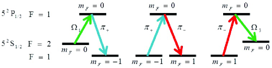
Figure 8: Experimental atomic configuration used to generate tripartite GHZ state. Here, $\Omega_{1}$ and $\Omega_{3}$ are the classical fields, and $\pi_{+}$ and $\pi_{-}$ are the quantized cavity modes with different polarizations, respectively.

Where the first (third) atom is coupled resonantly to an external $\pi$-polarized classical field and a $\pi_{+}$ ($\pi_{-}$) polarized photon modes of the cavity, and the middle atom is coupled resonantly to a $\pi_{+}$ and a $\pi_{-}$ polarized modes. Based on the above discussions, in order to obtain fidelity larger than 90%, one should keep the decay rate $\gamma<0.0055g$. This condition can be satisfied in recent experiments 37 ; 38 , wherein for an optical cavity with the wavelength about $850$ nm the parameters are set as: $g/2\pi=750$ MHz, $\gamma/2\pi=2.62$ MHz, $\kappa_{c}/2\pi=3.5$ MHz. Also, a near perfect fiber-cavity coupling with an efficiency larger than 99.9% can be realized using fiber-taper coupling to high-Q silica microspheres 39 . The fiber loss at the $852$ nm wavelength is about $2.2$ dB/km 40 , which corresponds to the fiber decay rate $1.52\times 10^{5}$ Hz. With these parameters, it seems that the present entanglement-generation scheme with a high fidelity larger than 93% could be feasible with the present experimental technique. The duration of the Zeno pulses $\Omega_{1}$ and $\Omega_{3}$ utilized to generate the desirable three-atom GHZ state can be estimated as $\pi/N_{1}\sqrt{\Omega_{1}^{2}+\Omega_{3}^{2}}\approx 1.43\times 10^{-8}$s, which is easily implemented for the present laser technology.

In conclusion, we have proposed an approach to achieve three-atom GHZ states by taking advantage of quantum Zeno dynamics. In present proposal, only one step operation is required to complete the generation. The generation of the GHZ states is controllable, as the proposed quantum Zeno dynamics can be switched on/off by controlling the classical drivings of the atoms at two ends. We note also that, the generated GHZ state is no longer evolving, at least theoretically, after switching off the classical drivings of the atoms at two-side cavities. Additionally, the evolution of system is always kept in the subspace with null-excitation of cavity fields. So, the scheme is immune to the decay of cavity modes. Moreover, the scheme loosens the requirement of strong cavity-fiber coupling. We also show that the proposal can be easily generalized to prepared the N-atom entanglement without increasing the number of the applied classical fields.

References

• (1) Introduction to Quantum Computation and Information, edited by H.-K. Lo, S. Popescu, and T. Spiller (World Scientific, Singapore, 1997).
• (2) M. A. Nielsen and I. L. Chuang, Quantum Computation and Quantum Information (Cambridge University Press, Cambridge, 2000).
• (3) C. H. Bennett and D. P. DiVincenzo, Nature (London) 404, 247 (2000).
• (4) A. K. Ekert, Phys. Rev. Lett. 67, 661 (1991).
• (5) D. M. Greenberger, M. A. Horne, A. Shimony and A. Zeilinger, Am. J. Phys 58, 1131 (1990).
• (6) M. Hillery, V. Buzek, and A. Berthiaume, Phys. Rev. A 59, 1829 (1999).
• (7) X.-B. Zou, K. Pahlke, and W. Mathis, Phys. Rev. A 68, 024302 (2003).
• (8) K. Pahlke, X.-B. Zou, and W. Mathis, J. Opt. B Quantum Semiclass. Opt. 6, S142 (2004).
• (9) D. Gonta, S. Fritzsche, and T. Radtke, Phys. Rev. A 77, 062312 (2008).
• (10) L. F. Wei, Y. X. Liu, and F. Nori, Phys. Rev. Lett 96, 246803 (2006).
• (11) R. J. Nelson, D. G. Cory, and S. Lloyd, Phys. Rev. A 61, 022106 (2000).
• (12) D. Leibfried et al., Nature (London) 438, 639 (2005).
• (13) M. Neeley et al., Nature (London) 467, 570 (2010).
• (14) J.M. Raimond, M. Brune, and S. Haroche, Rev. Mod. Phys. 73, 565 (2001).
• (15) J. I. Cirac and P. Zoller, Phys. Rev. A 50, R2799 (1994).
• (16) J. Hong and H.-W. Lee, Phys. Rev. Lett. 89, 237901 (2002).
• (17) J. I. Cirac, P. Zoller, H. J. Kimble, and H. Mabuchi, Phys. Rev. Lett. 78, 3221 (1997).
• (18) S. van Enk, J. Cirac, and P. Zoller, Phys. Rev. Lett. 78, 4293 (1997).
• (19) S. Bose, P. L. Knight, M. B. Plenio, and V. Vedral, Phys. Rev. Lett. 83, 5158 (1999).
• (20) S. Lloyd, M. S. Shahriar, J. H. Shapiro, and P. R. Hemmer, Phys. Rev. Lett. 87, 167903 (2001).
• (21) A. S. Parkins and H. J. Kimble, Phys. Rev. A 61, 052104 (2000).
• (22) T. Pellizzari, Phys. Rev. Lett 79, 5242 (1997).
• (23) A. Serafini, S. Mancini, S. Bose, Phys. Rev. Lett. 96, 010503 (2006).
• (24) P. Peng, F.-L. Li, Phys. Rev. A 75, 062320 (2007).
• (25) Z.-Q. Yin, F.-L. Li, Phys. Rev. A 75, 012324 (2007).
• (26) S.-Y. Ye, Z.-R. Zhong, S.-B. Zheng, Phys. Rev. A 77, 014303 (2008).
• (27) Z.-B. Yang, S.-Y. Ye, A. Serafini, S.-B.Zheng, J. Phys. B: At. Mol. Opt. Phys. 43, 085506 (2010).
• (28) X.-Y. Lv, L.-G. Si, X.-Y. Hao, and X. Yang, Phys. Rev. A 79, 052330 (2009).
• (29) S. B. Zheng, Eur. Phys. J. D 54, 719 (2009).
• (30) A. Zheng, and J. Liu, J. Phys. B: At. Mol. Opt. Phys. 44, 165501 (2011).
• (31) X.-Y. Lv, P.-J. Song, J.-B. Liu, and X. Yang, Opt. Express 17. 14298 (2009).
• (32) P.-B. Li, and F.-L. Li, Opt. Express 19, 1207-1216 (2011)
• (33) P. Facchi, V. Gorini, G. Marmo, S. Pascazio and E. C. G. Sudarshan, Phys. Lett. A 275, 12 (2000).
• (34) P. Facchi, S. Pascazio, Phys. Rev. Lett. 89, 080401 (2002).
• (35) P. Facchi, G. Marmo and S. Pascazio, J. Phys: Conf. Ser. 196, 012017 (2009).
• (36) P. Facchi, S. Pascazio, A. Scardicchio and L. S. Schulman, Phys. Rev. A 65, 012108 (2002).
• (37) A. Luis, Phys. Rev. A 63, 052112 (2001).
• (38) X. B. Wang, J. Q. You and F. Nori, Phys. Rev. A 77, 062339 (2008).
• (39) W.-A. Li, and G.-Y. Huang, Phys. Rev. A. 83, 022322 (2011).
• (40) A. Beige, D. Braun, B. Tregenna and P. L. Knight, Phys. Rev. Lett. 85, 1762-1765 (2000).
• (41) J. D. Franson , B. C. Jacobs and T. B. Pittman, Phys. Rev. A. 70, 062302 (2004).
• (42) X.-Q. Shao, L. Chen, S Zhang and K.-H. Yeon, J. Phys. B: At. Mol. Opt. Phys. 42, 165507 (2009).
• (43) J. D. Franson, T. B. Pittman and B. C. Jacobs, J. Opt. Soc. Am. B 24, 209 (2007).
• (44) L. F. Wei, Yu-xi Liu, and F. Nori, Phys. Rev. B 72, 104516 (2005).
• (45) S. M. Spillane, T. J. Kippenberg, K. J. Vahala, K. W. Goh, E. Wilcut, H. J. Kimble, Phys. Rev. A 71 013817 (2005).
• (46) J. R. Buck, H. J. Kimble, Phys. Rev. A 67 033806 (2003).
• (47) S. M. Spillane, T. J. Kippenberg, O. J. Painter, K. J. Vahala, Phys. Rev. Lett. 91 043902 (2003).
• (48) K. J. Gordon, V. Fernandez, P. D. Townsend, G. S. Buller, IEEE J. Quantum Electron. 40 900 (2004).