A non-perturbative renormalization group study of the stochastic Navier–Stokes equation

Abstract

We study the renormalization group flow of the average action of the stochastic Navier–Stokes equation with power-law forcing. Using Galilean invariance we introduce a non-perturbative approximation adapted to the zero frequency sector of the theory in the parametric range of the Hölder exponent $4-2\,\varepsilon$ of the forcing where real-space local interactions are relevant. In any spatial dimension $d$, we observe the convergence of the resulting renormalization group flow to a unique fixed point which yields a kinetic energy spectrum scaling in agreement with canonical dimension analysis. Kolmogorov’s $-5/3$ law is, thus, recovered for $\varepsilon=2$ as also predicted by perturbative renormalization. At variance with the perturbative prediction, the $-5/3$ law emerges in the presence of a saturation in the $\varepsilon$-dependence of the scaling dimension of the eddy diffusivity at $\varepsilon=3/2$ when, according to perturbative renormalization, the velocity field becomes infra-red relevant.

Kolmogorov’s K41 theory Ko41 ; Ko41a is the cornerstone of current understanding of fully developed turbulence in Newtonian fluids. A modern formulation of the theory Frisch95 is based on the asymptotic solution of the Kármán-Howarth-Monin equation, expressing energy balance, for stochastic incompressible Navier–Stokes equation

$$(\partial_{t}+\boldsymbol{v}\cdot\partial_{\boldsymbol{x}}-\kappa\partial_{\boldsymbol{x}}^{2})\boldsymbol{v}=\boldsymbol{f}-\partial_{\boldsymbol{x}}P\ ,$$ (1)

with $\boldsymbol{f}$ Gaussian, incompressible, zero average time-decorrelated with correlation

$$\prec\,\boldsymbol{f}(\boldsymbol{x}_{1},t_{1})\otimes\boldsymbol{f}(\boldsymbol{x}_{2},t_{2})\,\succ=\delta(t_{12})\,\mathsf{F}(\boldsymbol{x}_{12})\ .$$ (2)

Here $\prec\,\,\succ$ denotes the ensemble average, $\otimes$ the tensor product, $\boldsymbol{x}_{ij}:=\boldsymbol{x}_{i}-\boldsymbol{x}_{j}$, $t_{ij}:=t_{i}-t_{j}$ and $P$ is a pressure term enforcing incompressibility: $\partial_{\boldsymbol{x}}\cdot\boldsymbol{v}=0$. The solution of Kármán-Howarth-Monin equation predicts in any spatial dimension strictly larger than two that the energy injected by the external stirring ($\boldsymbol{f}$) around a typical spatial scale $L$ is conserved across an inertial range of scales through a constant-flux transfer mechanism, the “energy cascade”, before being dissipated by molecular viscosity. In two dimensions, energy and enstrophy conservation across the inertial range calls for a distinct analysis of the Kármán-Howarth-Monin equation Be99 ; Be00 ; Li96 formalizing the ideas introduced by Kraichnan in Kr67 . The solution predicts a constant flux inverse energy cascade from the injection scale towards the fluid integral scale. Below the injection scale a constant flux enstrophy cascade towards the dissipative scale may take place (see e.g. Bo07 ). The very existence and properties of the enstrophy cascade are, however, sensitive to the boundary conditions imposed on (1) and the eventual presence and shape of large scale friction mechanisms NaAnGuOt99 ; Be99 ; CoRa07 . Dimensional considerations based on the solution of the Kármán-Howarth-Monin equation lead then to scaling predictions for statistical indicators of the flow, including the $-5/3$ exponent for the $3d$ kinetic energy spectrum. These predictions convincingly account for a wide range of experimental and numerical observations (see e.g. Frisch95 ; Falkovich and references therein). Their first-principle derivation is therefore a well-grounded research question. A useful tool to pursue this goal is offered by the renormalization group, although its application to the inquiry of Navier–Stokes turbulence is ridden by challenges. Renormalization group analysis FoNeSt76 ; FoNeSt77 ; DeMa79 can be applied only far from the turbulent regime and for a very special choice of the random Gaussian field $\boldsymbol{f}$. This latter needs to have in any spatial dimension $d$ a power-law spectrum with Hölder exponent $4-2\,\varepsilon$:

$$\mathsf{F}(\boldsymbol{x}_{12};m,M)=$$ (3a)

$$\int_{\mathbb{R}^{d}}\frac{d^{d}p}{(2\,\pi)^{d}}\frac{e^{\imath\,\boldsymbol{p}\cdot\boldsymbol{x}_{12}}\,\,\mathsf{T}(\boldsymbol{p})}{d-1}\,\check{F}(\boldsymbol{p};m,M)\ ,$$

$$\check{F}(\lambda\,\boldsymbol{p};\lambda\,m\,,\lambda\,M)=\lambda^{4-d-2\varepsilon}\check{F}(\boldsymbol{p};m,M)\ ,$$ (3b)

with $\mathsf{T}(\boldsymbol{p})=\mathsf{I}-\boldsymbol{p}\otimes\boldsymbol{p}/p^{2}$ the transverse projector, $p:=\parallel\boldsymbol{p}\parallel$, and $m\ll M$ respectively the inverse integral and ultra-violet scales of the forcing. The rationale for the choice is that for vanishing $\varepsilon$ the canonical scaling dimensions of the convective (i.e. $\partial_{t}\boldsymbol{v}$, and $\boldsymbol{v}\cdot\partial_{\boldsymbol{x}}\boldsymbol{v}$) and dissipative (i.e. $\partial_{\boldsymbol{x}}^{2}\boldsymbol{v}$) terms in the Navier–Stokes equation tend to the same value. This fact suggests that for $\varepsilon$ equal zero canonical scaling dimensions may coincide with the exact scaling dimensions. In this sense, the vanishing $\varepsilon$ case defines a marginal scaling limit around which it may be possible to determine scaling dimensions by means of a perturbative expansion in $\varepsilon$ in analogy to what is done for critical phenomena described by a Boltzmann equilibrium (see e.g. Zinn ; Cardy96 ). For the stochastic Navier–Stokes equation the situation is, however, not conclusive. Renormalization group yields in any spatial dimension a kinetic energy spectrum

$$\mathcal{E}(p)\propto p^{\eta_{2:0}}\,,\hskip 28.45274pt\eta_{2:0}=1-4\varepsilon/3$$ (4)

DeMa79 (see also AdAnVa99 for an exhaustive review). In (4) the exponent labeling emphasizes the possibility of sub-leading corrections. Fully developed turbulence in $3d$ should correspond to an infra-red dominated spectrum of the stirring force as it occurs for $\varepsilon\geq 2$. Interestingly, (4) recovers Kolmogorov’s result for $\varepsilon$ equal two. Consistence with Kolmogorov theory then requires the exponent in (4) to freeze for $\varepsilon$ larger than two to the value $-5/3$. Within the perturbative renormalization group framework, the occurrence of such non-analytic behavior can only be argued FoFr83 . Direct numerical simulations SaMaPa98 ; BiCeLaSbTo04 exhibited, within a $512^{3}$-lattice accuracy, a transition in the $\varepsilon$-dependence of $\eta_{2}$ which is consistent with the freezing scenario. The situation is, however, completely different in two dimensions MaMGMu07 ; MaMGMu09 . On the one hand, perturbative renormalization group analysis Ho98 upholds the validity of (4) for any $\varepsilon$. On the other hand, the asymptotic solution of the Kármán-Howarth-Monin equation MaMGMu09 shows that (4) is always sub-dominant with respect to the inverse energy cascade spectrum $\mathcal{E}(p)\propto p^{-5/3}$, for $\varepsilon\leq 2$ i.e. even in the regime where renormalization group analysis should apply. Direct numerical simulations up to $2048^{2}$ resolution give clear evidence of the inverse cascade MaMGMu07 ; MaMGMu09 . A scenario reconciling these findings may be that the Kraichnan-Kolmogorov inverse cascade corresponds to a renormalization group non-perturbative fixed point which does not bifurcate from the Gaussian fixed point at marginality. Evidences of the occurrence of such an “exotic” phenomenon, have been given in models of wetting transitions by “non-perturbative approximations” of the Wilsonian renormalization group LiFi86 ; LiFi87 . More recently, similar methods gave evidence of the existence of a strong coupling fixed point in the Kardar-Parisi-Zhang model of interfacial growth CaChDeWs09 , yielding scaling predictions favorably comparing with direct numerical simulations. Motivated by these results, in the present contribution we derive the exact renormalization group equations for the stochastic Navier–Stokes equation. We then investigate them using a “non-perturbative approximations” similar to the one used in CaChDeWs09 . By this we mean, as often done in non-perturbative renormalization BeTeWe02 ; BaBe01 , truncations of the flow equations based on some assumption on the physical properties of the inquired system. Specifically, we investigate the consequences of the simplest closure compatible with Galilean invariance and with the number of relevant interactions identified by perturbative renormalization at small $\varepsilon$. The second requirement guarantees the existence of a limit where the closure becomes exact in the sense that it recovers the perturbative renormalization group fixed point. As in CaCh07 ; CaChDeWs09 , we focus on the exact renormalization group equations for the average action or thermodynamic potential defined by the stochastic Navier–Stokes equations. In striking contrast with the compressible stochastic dynamics studied in CaChDeWs09 , we do not find any evidence of a non-perturbative fixed point which may be associated to constant flux solutions in general and to the two dimensional inverse cascade in particular. The truncation we consider reproduces instead the expected correct scaling behavior in the regime dominated by real-space local interactions i.e. $d=3$ and $\varepsilon\,\leq 3/2$. Interestingly, we observe in any dimension a transition at $\varepsilon=3/2$ in the scaling behavior of the eddy-diffusivity. This latter deviates from the renormalization group scaling prediction by freezing from there on in $\varepsilon$ to its $\varepsilon=3/2$ value. This result was previously derived by different methods in MoWe95 . It is worth noticing that $\varepsilon=3/2$ is the threshold value after which the critical dimension of the stochastic Navier–Stokes velocity predicted by perturbative renormalization becomes negative or, in other words, infra-red relevant. In spite of the eddy diffusivity saturation, we obtain a kinetic energy spectrum scaling in agreement to (4) with no saturation for $\varepsilon\,>\,2$. This latter fact is not entirely surprising since the particle irreducible vertices contributing to the approximated renormalization group flow, are only a subset of those needed to fully reconstruct the flux i.e. the chief statistical indicator in Kolmogorov’s theory.

The structure of the paper is as follows. In section I we briefly recall the Kármán-Howarth-Monin equation and its predictions for power law forcing. In section II we derive the exact renormalization group average action for the model. The scope of these sections is to provide basic background on turbulence and functional renormalization to facilitate the reading by researchers familiar with one of these subjects but not the other. Using the Ward identities imposed by Galilean and translational invariance in section III we introduce our approximations of the exact flow. We write the resulting equations in section IV where we also outline their qualitative analysis. To simplify the discussion we detail auxiliary formulas in appendix C. An advantage of our formalism is that by preserving the structure of the exact renormalization group flow it guarantees the “realizability” of the “closure” that we impose BoKrOt93 . In V we describe the analytic solution of our equations in a simplified limit. Section VI reports the result of the numerical integration of our equations respectively in the three and two-dimensional cases. Finally we turn in VII to discussion and conclusions.

I Scaling predictions based on the Kármán-Howarth-Monin equation

The Kármán-Howarth-Monin equation describes the energy balance in the putative unique steady-state to which Galilean invariant statistical indicators are expected to converge. Specifically, if we consider the two-point equal time correlation tensor

$$\mathsf{C}_{2}(\boldsymbol{x}_{12},t)=\prec\,\boldsymbol{v}(\boldsymbol{x}_{1},t)\otimes\boldsymbol{v}(\boldsymbol{x}_{2},t)\,\succ\ ,$$ (5)

and the three point equal time structure tensor

$$\mathsf{S}_{3}(\boldsymbol{x}_{12},t)=\prec\,\delta\boldsymbol{v}\left(\boldsymbol{x}_{12},t\right)\otimes\delta\boldsymbol{v}\left(\boldsymbol{x}_{12}\right)\otimes\delta\boldsymbol{v}\left(\boldsymbol{x}_{12}\right)\succ\ ,$$ (6)

$$\delta\boldsymbol{v}\left(\boldsymbol{x}_{12}\right):=\boldsymbol{v}(\boldsymbol{x}_{1},t)-\boldsymbol{v}(\boldsymbol{x}_{2},t)\ ,$$ (7)

a straightforward calculation using incompressibility and the inertial range translational and parity invariance yields

$$\partial_{t}C+\frac{1}{2}\partial_{\boldsymbol{x}}\cdot\boldsymbol{S}-2\,\kappa\,\partial_{\boldsymbol{x}}^{2}C=F\ ,$$ (8)

for $C:=\mathrm{tr}\,\mathsf{C}_{2}$, $F:=\mathrm{tr}\,\mathsf{F}$ and $S^{\alpha}:=\mathsf{S}_{3\hskip 8.5359pt\alpha_{1}}^{\alpha\alpha_{1}}$ and Einstein convention on repeated indices. In any spatial dimension strictly larger than two, (8) admits an asymptotic solution under the hypotheses (see e.g. Frisch95 for a detailed discussion) that (i-1) statistical indicators attain a unique steady state and hence $\partial_{t}C=0$, (ii-1) they are smooth for any finite molecular viscosity but (iii-1) the inviscid limit of the energy dissipation exhibits a dissipative anomaly

$$0\,<\,-2\,\lim_{\kappa\downarrow 0}\lim_{\parallel\boldsymbol{x}\parallel\downarrow 0}\kappa\,\partial_{\boldsymbol{x}}^{2}C\neq-2\,\lim_{\parallel\boldsymbol{x}\parallel\downarrow 0}\lim_{\kappa\downarrow 0}\kappa\,\partial_{\boldsymbol{x}}^{2}C=0\ .$$ (9)

Under these hypotheses, if the dominant contribution to the forcing correlation comes from wave numbers of the order $m$, Kolmogorov’s classical result Ko41

$$\lim_{\parallel\boldsymbol{x}\parallel\downarrow 0}\lim_{\kappa\downarrow 0}\partial_{x^{\beta}}\mathsf{S}_{3}^{\alpha_{1}\alpha_{2}\alpha_{3}}(\boldsymbol{x})$$  , (10)

$$=-\,\frac{2\,\bar{E}}{d\,(d+2)}\mathcal{P}_{\boldsymbol{\alpha}}\left\{\delta^{\beta\alpha_{1}}\delta^{\alpha_{2}\alpha_{3}}\right\}\ ,$$

holds true for $m\parallel\boldsymbol{x}\parallel\,\ll\,1$, $\mathcal{P}_{\boldsymbol{\alpha}}$ being the index cyclical permutation operation over $\boldsymbol{\alpha}=(\alpha_{1},\alpha_{2},\alpha_{3})$ and, in accordance with Kolmogorov’s notation Ko41 ; Ko41a , $\bar{E}=F(0)/2$ the mean dissipation of energy . In other words, the leading scaling exponent of (6) is

$$\zeta_{3:0}=1\ .$$ (11)

Dimensional considerations then yield for the kinetic energy spectrum scaling exponent the Kolmogorov’s scaling law

$$\eta_{2:0}=-5/3\ .$$ (12)

If instead the forcing correlation is a power-law within the range of scales $M^{-1}\ll\parallel\boldsymbol{x}\parallel\ll m^{-1}$ with Hölder exponent $4-2\,\varepsilon$, we should distinguish two situations. If $\varepsilon\,<\,2$, the forcing correlation (3) remains well-defined in the limit of infinite integral scale $m^{-1}$. In such a case (10) holds for $M^{-1}\ll\parallel\boldsymbol{x}\parallel\,\ll\,\ell$ where we introduced $\ell=\kappa\,/\sqrt{F(0)}$, the typical scale below which molecular dissipation dominates. Under the present hypotheses $\ell\propto\kappa\,M^{\varepsilon-2}$, the omitted proportionality factor being a dimensional constant independent of $\kappa$ and $M$. This range of scales is not accessible by perturbative ultra-violet renormalization group methods. These latter may describe instead the range $\parallel\boldsymbol{x}\parallel\,\gg\,M^{-1}$ where the asymptotic solution of (8) states that the leading scaling exponent of (6) is

$$\zeta_{3:0}=-3+2\varepsilon\ .$$ (13)

Dimensional analysis based on (13) then recovers the renormalization group prediction (4) for the kinetic energy spectrum. A different scenario occurs for $\varepsilon\,>\,2$: the forcing correlation has a finite limit if the ultra-violet scale $M$ tends to infinity for any finite value of the inverse integral scale $m$. In the range $m^{-1}\,\ll\,\parallel\boldsymbol{x}\parallel\,\ll\,\ell$, $\ell\propto\kappa\,m^{\varepsilon-2}$, (10) holds with possible sub-dominant terms with scaling dimension (13). To summarize, the hint coming from the Kármán-Howarth-Monin equation for spatial dimensions $d\,>\,2$ is that the $-5/3$ exponent stems from the dominance for $\varepsilon\,>\,2$ of the constant flux over the dimensional scaling asymptotic solution of (8). This result can be justified within perturbative renormalization theory using an argument proposed by Fournier and Frisch in FoFr83 (see also AdAnVa99 ). It is worth here to briefly recall this argument in order to evince the assumptions on which it relies. Let $\check{C}(\boldsymbol{p})$ be the Fourier transform of the trace of the two-point equal time correlation tensor (5). Renormalization group analysis upholds that the expansion in powers of $\varepsilon$ can be re-summed in the form

$$\check{C}(p)\overset{M\uparrow\infty}{\to}\nu^{2}(p)\,p^{2-d}\,c\left(\frac{m}{p},\varepsilon\right)$$ (14)

Here, $c$ is a function independent of $M$ which can be determined order by order in a regular expansion around the renormalized theory (the so called “renormalized perturbation theory”). The $\nu(p)$ in the prefactor is the “running viscosity” the explicit form whereof within all orders in $\varepsilon$ is the main achievement of renormalization group analysis:

$$\nu(p)=\left[\frac{F(0)\,m_{\star}^{2\,\varepsilon-4}}{p^{2\,\varepsilon}}\right]^{1/3}$$ (15)

A crucial role here is played by the mass scale $m_{\star}$. Since for $\varepsilon\,<\,2$ the theory is well-defined in the limit of infinite integral scale, $m_{\star}$ in this range must have a finite limit as $m$, the inverse integral scale, tends to zero. For $\varepsilon\,>\,2$, on the contrary, the energy input becomes infra-red dominated and as a consequence $m_{\star}\propto m$. Finally, let us observe following FoFr83 ; AdAnVa99 that comparison with Kolmogorov theory should be done by holding fixed the energy input while taking the limit of infinite integral scale. Let us assume that: A the resummation (14) holds for any finite $\varepsilon$ and, B (14) admits a finite limit as the integral scale $m^{-1}$ tends to infinity. Under these hypotheses it follows immediately that

$$\lim_{\begin{subarray}{c}m\downarrow 0\\ F(0)=\mathrm{constant}\end{subarray}}\lim_{M\uparrow\infty}C(p)\sim\left\{\begin{array}[c]{ll}p^{2-4\varepsilon/3-d}&\hskip 5.69046pt\varepsilon\,<\,2\\ p^{2-8/3-d}&\hskip 5.69046pt\varepsilon\,>\,2\end{array}\right.$$ (18)

Note that (18) is equivalent to say that $c$ is finite in the limits for $\varepsilon\,<\,2$ and divergent for $\varepsilon\,>\,2$. Two mechanisms may obviously invalidate this result. Assumption A breaks down if for some finite $\varepsilon$ a new fixed point of the renormalization group transformation appears. This may lead to a different result for the running viscosity (15) marking the onset of a different critical regime. Glazek and Wilson gave in GlWi04 an analytically tractable example of a non-perturbative bifurcation of renormalization group flow fixed point. Scenarios for the break-down of A were already discussed in DeMa79 . Checking the validity of assumption B requires controlling the function $c$ in (14) in the limit of vanishing $m$. The needed technical tool is the so-called operator-product-expansion Zinn ; Cardy96 . In particular, $c$ may become divergent for $m\downarrow 0$ above some threshold value $\varepsilon_{\star}\,<\,2$ as some irrelevant composite operator contributing to $\check{C}$ turns relevant. Examples of such operators are known AdAnVa99 : the velocity field and its integer powers become relevant at $\varepsilon=3/2$ the energy dissipation at $\varepsilon=2$. In summary, the domain of validity in $3d$ of the renormalization group predictions and, even more, the exponent “freezing” needed to recover Kolmogorov theory are open research questions which we set out explore in the present contribution.

The asymptotic analysis of (8) in $2d$ must be treated apart in order to take into account enstrophy conservation. In particular Be99 ; Be00 , Kraichnan’s theory Kr67 is epitomized by a more restrictive version of (i-1), which we will refer to as (i-2), requiring only Galilean invariant quantities to reach a steady state. In other words, $\partial_{t}C$ does not vanish. Furthermore, (iii-1) is replaced by a new hypothesis (iii-2) ruling out the occurrence of dissipative anomaly for the kinetic energy dissipation:

$$\lim_{\kappa\downarrow 0}\lim_{\parallel\boldsymbol{x}\parallel\downarrow 0}\kappa\,\partial_{\boldsymbol{x}}^{2}C=\lim_{\parallel\boldsymbol{x}\parallel\downarrow 0}\lim_{\kappa\downarrow 0}\kappa\,\partial_{\boldsymbol{x}}^{2}C=0\ .$$ (19)

It is worth noticing that (iii-2) can be rigorously proved to hold true in some setup for the deterministic Navier–Stokes CoRa07 (see also discussion in Ku09 ). We refer the reader to MaMGMu09 for a detailed analysis of the two-dimensional Kármán-Howarth-Monin equation in the power-law case also corroborated by direct numerical simulations of (1). Here we only summarize the results. In the range of scales which can be investigated by perturbative ultra-violet renormalization group methods, three distinct regimes may set in depending upon the value of $\varepsilon$. For $\varepsilon\,<\,2$, the ultra-violet cut-off gives the dominant contribution to the total energy $F(0)\propto M^{4-2\,\varepsilon}$ and enstrophy $-(\partial_{\boldsymbol{x}}^{2}F)(0)\propto M^{6-2\,\varepsilon}$. Correspondingly, the inviscid limit in the range $M\,\parallel\boldsymbol{x}\parallel\,\gg\,1$ predicts for the leading and sub-leading scaling exponents of (6)

$$\zeta_{3:0}=1\hskip 28.45274pt\&\hskip 28.45274pt\zeta_{3:1}=-3+2\,\varepsilon\ .$$ (20)

This is in agreement with Kraichnan’s theory which predicts the onset of an inverse energy cascade for wave-numbers smaller than the one characteristic of the (total) input. The ensuing dimensional prediction for the kinetic energy spectrum scaling exponent is (12) while $\eta_{2:1}=1-4/3\varepsilon$ only describes a sub-leading correction. For $2\,<\,\varepsilon\,<\,3$, $F(0)\propto m^{4-2\,\varepsilon}$ and $-(\partial_{\boldsymbol{x}}^{2}F)(0)\propto M^{6-2\,\varepsilon}$ indicate that in the region $m^{-1}\,\gg\,\parallel\boldsymbol{x}\parallel\,\gg\,M^{-1}$ the third order structure tensor is sustained by an input of enstrophy from larger wave-numbers and an input of energy from smaller wave-numbers. As a result, the flux balances locally in real space with the forcing so that (13) holds true. Finally for $\varepsilon\,>\,3$ and in the presence of a large-scale hypo-friction MaMGMu09 both energy $F(0)\propto m^{4-2\,\varepsilon}$ and enstrophy$-(\partial_{\boldsymbol{x}}^{2}F)(0)\propto m^{6-2\,\varepsilon}$ inputs are dominated by the infra-red mass scale $m$. As a consequence, a direct enstrophy cascade sets in for $m\parallel\boldsymbol{x}\parallel\,\ll\,1$ and

$$\zeta_{3:0}=3\hskip 28.45274pt\&\hskip 28.45274pt\zeta_{3:1}=-3+2\,\varepsilon\ .$$ (21)

Again, dimensional analysis based on (21) predicts

$$\eta_{2:0}=-3\hskip 28.45274pt\&\hskip 28.45274pt\eta_{2:1}=1-4/3\,\varepsilon\ ,$$ (22)

with the leading scaling exponent “freezing” at the threshold value attained at $\varepsilon=3$. With these results in mind, we turn now to the formulation of a non-perturbative renormalization group theory with the aim of collating scaling predictions for the energy spectrum.

II Renormalization group flow for the average action

II.1 Thermodynamic formalism

For finite infra-red $m$ and ultra-violet $M$ cut-offs of the Gaussian forcing (2) it is reasonable to assume that the generating function

$$\mathcal{Z}_{(\boldsymbol{\jmath},\bar{\boldsymbol{\jmath}})}:=\prec\,e^{\boldsymbol{\jmath}\star\boldsymbol{v}(;\boldsymbol{f}+\bar{\boldsymbol{\jmath}})}\,\succ\ ,$$ (23)

is well defined. The average in (23) is over the Gaussian statistics of the forcing, $\boldsymbol{v}(;\boldsymbol{f}+\bar{\boldsymbol{\jmath}})$ is the solution of (1) for any fixed realization of $\boldsymbol{f}$ shifted by an arbitrary source field $\bar{\boldsymbol{\jmath}}$, and $\star$ denotes the $\mathbb{L}^{2}\left(\mathbb{R}^{d}\times\mathbb{R}\right)$ scalar product

$$\boldsymbol{\jmath}\star\boldsymbol{v}(;\bar{\boldsymbol{\jmath}}):=\int_{\mathbb{R}^{d}\times\mathbb{R}}d^{d}x\,dt\,\boldsymbol{\jmath}\left(\boldsymbol{x},t\right)\cdot\boldsymbol{v}\left(\boldsymbol{x},t;\bar{\boldsymbol{\jmath}}\right)\ .$$ (24)

Functional derivatives at zero external sources $\left(\boldsymbol{\jmath},\bar{\boldsymbol{\jmath}}\right)$ of (23) yield the expressions of the correlation and response (to variations of $\boldsymbol{v}$ with respect to $\boldsymbol{f}$) tensors of any order. The generating function of connected correlations

$$\mathcal{W}_{(\boldsymbol{\jmath},\bar{\boldsymbol{\jmath}})}:=\ln\mathcal{Z}_{(\boldsymbol{\jmath},\bar{\boldsymbol{\jmath}})}\ ,$$ (25)

is equal to minus the free energy of the field theory. In particular, with these conventions we have

$$\mathsf{C}^{\alpha_{1}\alpha_{2}}(\boldsymbol{x}_{12},t_{12})\equiv\,[\mathsf{W}^{(2,0)}]^{\alpha_{1}\alpha_{2}}\left(\boldsymbol{x}_{12},t_{12}\right)$$ (26)

$$\hskip 42.67912pt:=\left.\frac{\delta^{2}\mathcal{W}_{\left(\boldsymbol{\jmath},\bar{\boldsymbol{\jmath}}\right)}}{\delta\jmath_{\alpha_{1}}(\boldsymbol{x}_{1},t_{1})\delta\jmath_{\alpha_{2}}(\boldsymbol{x}_{1},t_{2})}\right|_{\boldsymbol{\jmath}=\bar{\boldsymbol{\jmath}}=0}\ .\hskip 28.45274pt$$

Analogously, the second order response function is

$$\prec\,\frac{\delta v^{\alpha_{1}}(\boldsymbol{x}_{1},t_{1})}{\delta f^{\alpha_{2}}(\boldsymbol{x}_{2},t_{2})}\,\succ\equiv[\mathsf{W}^{(1,1)}]^{\alpha_{1}}_{\hskip 5.69046pt\alpha_{2}}\left(\boldsymbol{x}_{12},t_{12}\right)$$ (27)

$$\hskip 42.67912pt:=\left.\frac{\delta^{2}\mathcal{W}_{\left(\boldsymbol{\jmath},\bar{\boldsymbol{\jmath}}\right)}}{\delta\jmath_{\alpha_{1}}(\boldsymbol{x}_{1},t_{1})\delta\bar{\jmath}^{\alpha_{2}}(\boldsymbol{x}_{2},t_{2})}\right|_{\boldsymbol{\jmath}=\bar{\boldsymbol{\jmath}}=0}\ .\hskip 28.45274pt$$

The Legendre transform of the free energy (25) specifies the average action or the thermodynamic potential of the statistical field theory:

$$\mathcal{U}_{(\boldsymbol{u},\bar{\boldsymbol{u}})}:=\sup_{(\boldsymbol{\jmath}\,,\bar{\boldsymbol{\jmath}})}\left\{\boldsymbol{\jmath}\star\boldsymbol{u}+\bar{\boldsymbol{\jmath}}\star\bar{\boldsymbol{u}}-\mathcal{W}_{(\boldsymbol{\jmath}\,,\bar{\boldsymbol{\jmath}})}\right\}\ .$$ (28)

The Legendre anti-transform of (28) reconstruct the convex envelope of the free energy (25). In this sense the average action may be interpreted as an ultra-violet regularization of the theory. The average action is a functional of the fields $\left(\boldsymbol{u},\bar{\boldsymbol{u}}\right)$, which are Legendre conjugate to the external sources $\left(\boldsymbol{\jmath},\bar{\boldsymbol{\jmath}}\right)$ and which as customary will be referred to as “classical fields”. As extensively discussed in WE91 ; BeTeWe02 the average action provides a convenient starting point for non-perturbative renormalization. Dealing with it is conceptually equivalent to working with the Wilsonian effective action as done by Polchinski in Po83 . Namely, the corresponding equations can in principle be converted in one another by a Legendre transform if one identifies the running cut-off. The average action offers, as we will see below, some technical advantages BaBe01 which significantly simplify the formalism.

II.2 Flow equations

A stationary phase approximation to (23) in the weak stirring limit $\mathsf{F}\downarrow 0$ (see appendix B) yields with logarithmic accuracy

$$\mathcal{U}_{M}\sim$$ (29a)

$$\bar{\boldsymbol{u}}\star[(\partial_{t}-\kappa\,\partial_{x}^{2})\boldsymbol{u}+\mathsf{T}(\boldsymbol{u}\cdot\partial_{\boldsymbol{x}}\boldsymbol{u})]-\frac{\bar{\boldsymbol{u}}\star\mathsf{F}\star\bar{\boldsymbol{u}}}{2}\ ,$$

$$\partial_{\boldsymbol{x}}\cdot\boldsymbol{u}=\partial_{\boldsymbol{x}}\cdot\bar{\boldsymbol{u}}=0\ .$$ (29b)

The limit $\mathsf{F}=0$ describes the trivial steady state of the decaying Navier-Stokes equation. We posit that (29) provides the initial condition for the renormalization group flow of the running average action $\mathcal{U}_{m_{r}}$. This flow describes the building up of the exact average action $\mathcal{U}$ of (23) as a function of an infra-red cut-off suppressing any interaction above an infra-red scale $m_{r}$ and recovering $\mathcal{U}$ in the limit of vanishing $m_{r}$. These conditions can be matched We93 ; BeTeWe02 if we replace in (1) the molecular viscosity with an “hyper-viscous” term, local in wave number space,

$$\kappa\mapsto\tilde{\kappa}:=\kappa+\kappa_{m_{r}}\check{R}\left(\frac{p}{m_{r}}\right)\ ,$$ (30)

with $\check{R}$ a function rapidly decaying for large values of its argument and diverging at the origin. A convenient choice CaChDeWs09 is

$$\check{R}(p)=\frac{1}{e^{p^{2}}-1}\ .$$ (31)

In (30) we also introduced the “running” viscosity $\kappa_{m_{r}}$. We will use this extra degree of freedom to constrain the flow to satisfy a renormalization condition on the eddy diffusivity. As for the viscosity, we then apply an high-pass filter to the Gaussian forcing

$$\boldsymbol{f}\mapsto\boldsymbol{\tilde{f}}\ ,$$ (32)

such that

$$\prec\,\boldsymbol{\tilde{f}}_{1}\otimes\boldsymbol{\tilde{f}}_{2}\,\succ=\delta(t_{12})\,\sum_{i=0}^{1}\mathsf{F}_{(i)}\left(\boldsymbol{x}_{12};m_{r}\right)\ ,$$ (33)

where we defined

$$\mathsf{F}_{(0)}\left(\boldsymbol{x}_{12};m_{r}\right)=\mathsf{F}\left(\boldsymbol{x}_{12};m_{r},\infty\right)\ ,$$ (34a)

$$\mathrm{tr}\,\check{\mathsf{F}}_{(0)}\left(\boldsymbol{p};m_{r}\right)=F_{o}\,m_{r}^{4-d-2\,\varepsilon}\,(d-1)\,\chi_{(0)}\left(\frac{p}{m_{r}}\right)\ ,$$ (34b)

and

$$\check{\mathsf{F}}_{(1)}\left(\boldsymbol{p};m_{r}\right)=F_{m_{r}}\chi_{(1)}(p;m_{r})\,\mathsf{T}(\boldsymbol{p})\ ,$$ (35a)

$$\chi_{(1)}(p;m_{r})\,:=\,p^{2}\,e^{-\frac{p^{2}}{m_{r}}}\ .$$ (35b)

This latter term describes a local (in the infra-red or for $m_{r}=O(M)$) perturbation of the measure progressively suppressed as $m_{r}$ decreases. Locality entitles us to interpret this term as a renormalization counter-term in the sense of HoNa96 ; Ho98 ; AdHoKoVa05 . Again, we will use the extra freedom introduced by $F_{m_{r}}$ to impose a renormalization condition on the flow. The replacements (30), (32) turn (23) into a family of generating functions differentiable with respect to the parameter $m_{r}$. A straightforward calculation (see appendix A.1) yields

$$m_{r}\partial_{m_{r}}\mathcal{Z}_{\left(\boldsymbol{\jmath},\bar{\boldsymbol{\jmath}}\right)}=\int_{\mathbb{R}^{d}\times\mathbb{R}^{d}\times\mathbb{R}}d^{d}x_{1}d^{d}x_{2}dt\,$$ (36)

$$\times\left\{\frac{(m_{r}\partial_{m_{r}}\tilde{\mathsf{F}})^{\alpha_{1}\alpha_{2}}(\boldsymbol{x}_{12})}{2}\frac{\delta^{2}\mathcal{Z}_{\left(\boldsymbol{\jmath},\bar{\boldsymbol{\jmath}}\right)}}{\delta\bar{\jmath}^{\alpha_{1}}(\boldsymbol{x}_{1},t)\delta\bar{\jmath}^{\alpha_{2}}(\boldsymbol{x}_{2},t)}\right.$$

$$\left.+(m_{r}\partial_{m_{r}}\kappa_{m_{r}}\,R)(\boldsymbol{x}_{12})\partial_{\boldsymbol{x}_{2}}^{2}\frac{\delta^{2}\mathcal{Z}_{\left(\boldsymbol{\jmath},\bar{\boldsymbol{\jmath}}\right)}}{\delta\bar{\jmath}^{\alpha_{1}}(\boldsymbol{x}_{1},t)\delta\jmath_{\alpha_{1}}(\boldsymbol{x}_{2},t)}\right\}\ .$$

Upon defining

$$\boldsymbol{\mathcal{R}}(\boldsymbol{x}_{12},t_{12}):=$$ (37)

$$\delta(t_{12})\begin{bmatrix}0&\kappa_{m_{r}}\mathsf{R}(\boldsymbol{x}_{12})\,\partial_{\boldsymbol{x}_{1}}^{2}\\ \kappa_{m_{r}}\mathsf{R}(\boldsymbol{x}_{12})^{\dagger}\,\overset{\leftarrow}{\partial_{\boldsymbol{x}_{1}}^{2}}&\tilde{\mathsf{F}}(\boldsymbol{x}_{12})\ ,\end{bmatrix}$$

and

$$\boldsymbol{\mathcal{W}}_{(\boldsymbol{\jmath},\bar{\boldsymbol{\jmath}})}^{(2)}(\boldsymbol{x}_{1},\boldsymbol{x}_{2},t_{1},t_{2}):=$$ (38)

$$\begin{bmatrix}\mathcal{W}_{(\boldsymbol{\jmath},\bar{\boldsymbol{\jmath}})}^{(2,0)}&\mathcal{W}_{(\boldsymbol{\jmath},\bar{\boldsymbol{\jmath}})}^{(1,1)}\\ \mathcal{W}_{(\boldsymbol{\jmath},\bar{\boldsymbol{\jmath}})}^{(1,1)\dagger}&\mathcal{W}_{(\boldsymbol{\jmath},\bar{\boldsymbol{\jmath}})}^{(0,2)}\end{bmatrix}\circ(\boldsymbol{x}_{1},\boldsymbol{x}_{2},t_{1},t_{2})\ ,$$

we can recast (36) into the form of an equation for the free energy which, in compact form, reads

$$m_{r}\partial_{m_{r}}\mathcal{W}_{\left(\boldsymbol{\jmath},\bar{\boldsymbol{\jmath}}\right)}=$$ (39)

$$\frac{1}{2}\mathrm{tr}\left\{(m_{r}\partial_{m_{r}}\boldsymbol{\mathcal{R}})\star\left(\boldsymbol{\mathcal{W}}_{\left(\boldsymbol{\jmath},\bar{\boldsymbol{\jmath}}\right)}^{(2)}-\boldsymbol{\mathcal{W}}_{\left(\boldsymbol{\jmath},\bar{\boldsymbol{\jmath}}\right)}^{(1)}\boldsymbol{\mathcal{W}}_{\left(\boldsymbol{\jmath},\bar{\boldsymbol{\jmath}}\right)}^{(1)}\right)\right\}\ .$$

Functional derivatives at zero sources of (39) spawn a hierarchy of equations satisfied by the full set of connected correlation of the theory. From (39) we derive the average action flow using the following two observations. First, the very definition of Legendre transform (28) implies

$$m_{r}\partial_{m_{r}}\mathcal{W}_{\left(\boldsymbol{\jmath},\bar{\boldsymbol{\jmath}}\right)}=-m_{r}\partial_{m_{r}}\mathcal{U}_{\left(\boldsymbol{u},\bar{\boldsymbol{u}}\right)}\ .$$ (40)

Second, the evaluation of (38) at zero sources restores translational invariance:

$$\boldsymbol{\mathsf{W}}^{(2)}(\boldsymbol{x}_{12},t_{12}):=\begin{bmatrix}\mathsf{W}^{(2,0)}&\mathsf{W}^{(1,1)}\\ \mathsf{W}^{(1,1)\dagger}&0\end{bmatrix}\circ(\boldsymbol{x}_{12},t_{12})\ .$$ (41)

The matrix elements of (41) are specified by the second order correlation and response functions (26), (27). We may refer to them as indicators of the “Gaussian” part of the statistics of (1). We can use (41) and the general relation

$$\boldsymbol{\mathrm{I}}=\boldsymbol{\mathcal{W}}_{(\boldsymbol{\jmath},\bar{\boldsymbol{\jmath}})}^{(2)}\star\boldsymbol{\mathcal{U}}_{(\boldsymbol{u},\bar{\boldsymbol{u}})}^{(2)}\ ,$$ (42)

following from the Legendre transform (28), to decouple the average action into a Gaussian and an interaction part BoDaMa94 :

$$\boldsymbol{\mathrm{I}}:=\boldsymbol{\mathcal{W}}_{(\boldsymbol{\jmath},\bar{\boldsymbol{\jmath}})}^{(2)}\star[\boldsymbol{\mathsf{W}}^{(2)-1}+\boldsymbol{\mathcal{U}}_{(\boldsymbol{u},\bar{\boldsymbol{u}})}^{(2)\,int}]\ .$$ (43)

Solving this latter relation for $\boldsymbol{\mathcal{W}}_{(\boldsymbol{\jmath},\bar{\boldsymbol{\jmath}})}^{(2)}$

$$\boldsymbol{\mathcal{W}}_{(\boldsymbol{\jmath},\bar{\boldsymbol{\jmath}})}^{(2)}=[\boldsymbol{\mathrm{I}}+\boldsymbol{\mathsf{W}}^{(2)}\star\boldsymbol{\mathcal{U}}_{(\boldsymbol{u},\bar{\boldsymbol{u}})}^{(2)int}]^{-1}\star\boldsymbol{\mathsf{W}}^{(2)}\ ,$$ (44)

allows us to finally derive the equation for the average action :

$$m_{r}\partial_{m_{r}}\left\{\mathcal{U}_{(\boldsymbol{u},\bar{\boldsymbol{u}})}-\frac{1}{2}[\boldsymbol{u}\,,\bar{\boldsymbol{u}}]\star(m_{r}\partial_{m_{r}}\boldsymbol{\mathcal{R}})\star\begin{bmatrix}\boldsymbol{u}\\ \bar{\boldsymbol{u}}\end{bmatrix}\right\}=$$ (45)

$$-\mathrm{tr}\,\frac{(m_{r}\partial_{m_{r}}\boldsymbol{\mathcal{R}})}{2}\star\left[\sum_{n=0}^{\infty}(-\boldsymbol{\mathsf{W}}^{(2)}\star\boldsymbol{\mathcal{U}}_{(\boldsymbol{u},\bar{\boldsymbol{u}})}^{(2)int})^{n}\right]\star\boldsymbol{\mathsf{W}}^{(2)}\ .$$

Some observations are in order. First, the flow equation (45) is effectively an equation for the reduced average action obtained by subtracting the quadratic counter-terms associated to the running infra-red cut-off. This is desirable because all physical information is indeed contained in the reduced average action. Second, the flow in (45) does not depend upon the theory under consideration which instead specify the initial conditions for the evolution. This is a formalization of Wilson’s idea of renormalization group as a flow in the space of the probability measures. The fixed point of the flow does not depend on the details of the microscopic theory used as initial condition for $m_{r}=M$. It depends instead upon the basin of attraction to which the initial condition belongs. Finally, solving (45) exactly is equivalent to solve an infinite non-close hierarchy of equations. Perturbative renormalization tells us, however, that there are only a finite number of relevant coupling, at most two for $\varepsilon\ll 1$ and $d\,\gtrsim\,2$ HoNa96 ; AdHoKoVa05 ; AdAnVa99 , determining the scaling properties of the stochastic Navier–Stokes (1). Based on this observation, we now turn to the derivation of a truncation of the right hand side of (45) in order to derive explicit scaling predictions.

III Galilean invariance and approximation

Perturbative renormalization identifies the number of relevant couplings by diagram power counting in unit of the ultra-violet cut-off Zinn . Relevant couplings correspond to proper vertices $\mathsf{U}^{(i,j)}$ proportional to powers of $M$ larger or equal than zero. For the stochastic Navier–Stokes equations only $\mathsf{U}^{(1,1)}$ for any $d$ and $\mathsf{U}^{(0,2)}$, for $d\,\gtrsim\,2$ have non-negative ultra-violet degree. We can use this information to hypothesize that (45) converges towards an average action of the form

$$\mathcal{U}_{(\boldsymbol{u},\bar{\boldsymbol{u}})}=\boldsymbol{u}\star\mathsf{U}^{(1,1)}\star\bar{\boldsymbol{u}}$$ (46)

$$+\frac{1}{2}\mathsf{U}^{(0,2)}(\star\bar{\boldsymbol{u}})^{2}+\frac{1}{2}(\boldsymbol{u}\star)^{2}\mathsf{U}^{(2,1)}\star\bar{\boldsymbol{u}}\ .$$

Clearly, the Ansatz closes the hierarchy of equations spawned by (45) since it is straightforward to verify that

$$\boldsymbol{\mathcal{U}}_{(\boldsymbol{u},\bar{\boldsymbol{u}})}^{(2)int}=\begin{bmatrix}\mathsf{U}^{(2,1)}\star\bar{\boldsymbol{u}}&\boldsymbol{u}\star\mathsf{U}^{(2,1)}\\ (\boldsymbol{u}\star\mathsf{U}^{(2,1)})^{\dagger}&0\end{bmatrix}\ ,$$ (47)

and by (28)

$$\mathsf{W}^{(1,1)}=\mathsf{U}^{(1,1)\dagger\,-1}\ ,$$ (48a)

$$\mathsf{W}^{(2,0)}=-\mathsf{W}^{(1,1)}\star\mathsf{U}^{(0,2)}\star\mathsf{W}^{(1,1)\dagger}\ .$$ (48b)

Note that

$$\mathcal{Z}_{\left(\boldsymbol{\jmath},\bar{\boldsymbol{\jmath}}\right)}^{(0,1)}(\boldsymbol{x},t)=\prec\,e^{\boldsymbol{\jmath}\star\boldsymbol{v}(\boldsymbol{f}+\bar{\boldsymbol{\jmath}})}\boldsymbol{\jmath}\star\frac{\delta\boldsymbol{v}(\boldsymbol{f}+\bar{\boldsymbol{\jmath}})}{\delta\ \bar{\boldsymbol{\jmath}}(\boldsymbol{x},t)}\,\succ\ ,$$ (49)

implies that $\mathsf{W}^{(0,i)}=\mathsf{U}^{(i,0)}=0$ for any integer $i$. To further evince the rationale behind (46) we observe that

$$\check{\mathsf{U}}^{(1,1)}(\boldsymbol{p}_{1},\omega_{1}|\boldsymbol{p}_{2},\omega_{2})=(2\,\pi)^{d+1}\,\delta^{(d)}(\sum_{i=1}^{2}\boldsymbol{p}_{i})$$ (50)

$$\times\,\delta(\sum_{i=1}^{2}\omega_{i})[\imath\,\omega_{1}+\kappa\,p_{1}^{2}\,g^{(1,1)}(p_{1},\omega_{1})]\,\mathsf{T}(\boldsymbol{p}_{1})\ ,$$

corresponds to a “dressing” of the quadratic coupling in (29). Differentiating with respect to $p_{1}^{2}$ at zero wave-number and frequency the translational invariant part of (50) provides a convenient non-perturbative definition of the eddy diffusivity. We will therefore refer to (50) as the “eddy diffusivity” vertex. Also the “interaction” vertex

$$\check{\mathsf{U}}(\boldsymbol{p}_{1},\omega_{1},\boldsymbol{p}_{2},\omega_{2}|\boldsymbol{p}_{3},\omega_{3})=$$ (51)

$$(2\,\pi)^{d+1}\,\delta^{(d)}(\sum_{i=1}^{3}\boldsymbol{p}_{i})\,\delta(\sum_{i=1}^{3}\omega_{i})\,\imath\,g^{(2,1)}(p_{1},\omega_{1},p_{2},\omega_{2})$$

$$\times\,\mathcal{P}_{(\boldsymbol{p}_{1},\boldsymbol{p}_{2})}\left\{\mathsf{T}(\boldsymbol{p}_{1})\cdot\mathsf{T}(\boldsymbol{p}_{3})\otimes\mathsf{T}(\boldsymbol{p}_{2})\cdot\boldsymbol{p}_{3}\right\}\ ,$$

admits a similar direct interpretation from (29). Finally, comparison with (29) evinces that the “force” vertex

$$\check{\mathsf{U}}^{(0,2)}(\boldsymbol{p}_{1},\omega_{1},\boldsymbol{p}_{2},\omega_{2})=$$ (52a)

$$-(2\,\pi)^{d+1}\,\delta^{(d)}(\sum_{i=1}^{2}\boldsymbol{p}_{i})\delta(\sum_{i=1}^{2}\omega_{i})\,g^{(0,2)}(p_{1},\omega_{1})\,\mathsf{T}(\boldsymbol{p}_{1})\ ,$$

$$g^{(0,2)}(p_{1},\omega_{1}):=$$ (52b)

$$\frac{1}{d-1}\sum_{i=0}^{1}\mathrm{tr}\,\check{\mathsf{F}}_{(i)}(p_{1},m_{r})+\tilde{g}^{(0,2)}(p_{1},\omega_{1})\ ,$$

describes (minus) the effective forcing correlation. The three vertices are, however, not completely independent. Galilean invariance constrains the average action to satisfy the Ward identity (see e.g. FrTa94 ; To97 ; CoTo97 and appendix A.2)

$$0=\ddot{\boldsymbol{r}}\star\boldsymbol{\bar{u}}+\frac{\delta\,\mathcal{U}}{\delta\boldsymbol{u}}\star\left(\boldsymbol{r}\cdot\boldsymbol{\partial}\boldsymbol{u}-\dot{\boldsymbol{r}}\right)+\frac{\delta\,\mathcal{U}}{\delta\bar{\boldsymbol{u}}}\star\boldsymbol{r}\cdot\boldsymbol{\partial}\bar{\boldsymbol{u}}\ ,$$ (53)

whence it follows after standard manipulations Zinn

$$\check{\mathsf{U}}^{(2,1)}(\boldsymbol{p}_{1},\omega_{1},\boldsymbol{0},0|\boldsymbol{p}_{3},\omega_{3})$$ (54)

$$=\boldsymbol{p}_{1}\partial_{\omega_{1}}\check{\mathsf{U}}^{(1,1)}(\boldsymbol{p}_{1},\omega_{1}|\boldsymbol{p}_{3},\omega_{3})\ .$$

In the context of perturbative renormalization (54) is used to show that if a parameter fine-tuning ensures that $\check{\mathsf{U}}^{(1,1)}$ is finite in the limit $M$ tending to infinity so must be $\check{\mathsf{U}}^{(2,1)}$. In general (54) is not sufficient to fully specify the form of the interaction vertex in terms of $\mathsf{U}^{(1,1)}$. If we, furthermore, hypothesize

$$g^{(2,1)}=1\ ,$$ (55)

then (54) implies

$$g^{(1,1)}(p_{1},\omega)=g^{(1,1)}(p)\ .$$ (56)

Such an approximation is too rough to give a self-consistent model for the full second order statistics. Our goal here is more restrictive as it is only to derive self-consistent scaling predictions at scales much larger than the dissipative. We therefore posit that (46) and (55) may serve for a self-closure able to capture the scaling behavior of the zero frequency sector of the theory. We also notice that a consequence of imposing (55), is that a generalized Taylor hypothesis Frisch95 is verified by the two point correlation function for which the dispersion relation

$$\omega=\imath\,\kappa\,p^{2}\,g^{(1,1)}(p)\ ,$$ (57)

holds true. As a final step in the derivation of our approximation we rewrite the vertices (50), (52a) to decouple explicitly the functional dependence on the cut-off. Thus, we couch the eddy-diffusivity vertex into the form

$$g^{(1,1)}(p;m_{r}):=\frac{\kappa_{m_{r}}}{\kappa}\left[\gamma^{(1,1)}\left(p;m_{r}\right)+\check{R}\left(\frac{p}{m_{r}}\right)\right]\ ,$$ (58)

where now $\gamma^{(1,1)}$ is an unknown non-dimensional function which our renormalization group equation will determine. Similarly we write

$$\tilde{g}^{(0,2)}(p;m_{r}):=$$ (59)

$$\left[\lambda_{(0)}\,m_{r}^{2-d-2\,\varepsilon}+\lambda_{(1)}\right]\,p^{2}\,\gamma^{(0,2)}\left(p;m_{r}\right)\ ,$$

where we defined the Grashof numbers

$$\lambda_{(0)}:=\frac{\Omega_{d}}{(2\,\pi)^{d}}\frac{F_{o}}{\kappa_{m_{r}}^{3}\,m_{r}^{2\,\varepsilon}}\ ,$$ (60a)

$$\lambda_{(1)}:=\frac{\Omega_{d}}{(2\,\pi)^{d}}\frac{F_{m_{r}}}{\kappa_{m_{r}}^{3}\,m_{r}^{2-d}}\ ,$$ (60b)

measuring the intensity of the non-local and local components of the stochastic forcing. In the context of perturbative renormalization the pair (60) specifies the running coupling constant of the model HoNa96 ; AdHoKoVa05 ; AdAnVa99 . In (60) we denoted

$$\Omega_{d}=\frac{2\,\pi^{d/2}}{\Gamma\left(\frac{d}{2}\right)}\ .$$ (61)

IV Approximated renormalization group flow

The Ansatz

$$\mathcal{U}_{(\boldsymbol{u},\bar{\boldsymbol{u}})}=\boldsymbol{u}\star\mathsf{U}^{(1,1)}\star\bar{\boldsymbol{u}}$$ (62)

$$+\frac{1}{2}\mathsf{U}^{(0,2)}(\star\bar{\boldsymbol{u}})^{2}+(\mathsf{T}\bar{\boldsymbol{u}})\cdot[(\mathsf{T}\boldsymbol{u})\cdot\boldsymbol{\partial}](\mathsf{T}\boldsymbol{u})\ ,$$

with $\mathsf{T}$ the transverse projector and (50), (52a) specifying the Fourier representation of the order two vertices summarizes the approximations described in the previous section. The insertion of (62) into the exact renormalization group equation (45) yields the equations

$$m_{r}\partial_{m_{r}}\left\{(d-1)\,\kappa_{m_{r}}\,p^{2}\,\gamma^{(1,1)}(p;m_{r})\right\}=$$ (63a)

$$-\frac{1}{2}\mathrm{tr}\left\{\widetilde{\boldsymbol{\mathsf{W}}^{(2)}}\star\frac{\delta\boldsymbol{\mathcal{U}}_{(\boldsymbol{u},\bar{\boldsymbol{u}})}^{(2)int}}{\delta\bar{u}_{\alpha_{1}}}\star\boldsymbol{\mathsf{W}}^{(2)}\star\frac{\delta\boldsymbol{\mathcal{U}}_{(\boldsymbol{u},\bar{\boldsymbol{u}})}^{(2)int}}{\delta u^{\alpha_{2}}}\right\}_{\omega=0}$$

$$-\frac{1}{2}\mathrm{tr}\left\{\boldsymbol{\mathsf{W}}^{(2)}\star\frac{\delta\boldsymbol{\mathcal{U}}_{(\boldsymbol{u},\bar{\boldsymbol{u}})}^{(2)int}}{\delta\bar{u}_{\alpha_{1}}}\star\widetilde{\boldsymbol{\mathsf{W}}^{(2)}}\star\frac{\delta\boldsymbol{\mathcal{U}}_{(\boldsymbol{u},\bar{\boldsymbol{u}})}^{(2)int}}{\delta u^{\alpha_{2}}}\right\}_{\omega=0}$$

$$m_{r}\partial_{m_{r}}\left\{(d-1)\,\tilde{g}^{(0,2)}(p;m_{r})\right\}=$$ (63b)

$$-\frac{1}{2}\mathrm{tr}\left\{\widetilde{\boldsymbol{\mathsf{W}}^{(2)}}\star\frac{\delta\boldsymbol{\mathcal{U}}_{(\boldsymbol{u},\bar{\boldsymbol{u}})}^{(2)int}}{\delta\bar{u}_{\alpha_{1}}}\star\boldsymbol{\mathsf{W}}^{(2)}\star\frac{\delta\boldsymbol{\mathcal{U}}_{(\boldsymbol{u},\bar{\boldsymbol{u}})}^{(2)int}}{\delta\bar{u}_{\alpha_{2}}}\right\}_{\omega=0}$$

$$-\frac{1}{2}\mathrm{tr}\left\{\boldsymbol{\mathcal{W}}^{(2)}\star\frac{\delta\boldsymbol{\mathcal{U}}_{(\boldsymbol{u},\bar{\boldsymbol{u}})}^{(2)int}}{\delta\bar{u}_{\alpha_{1}}}\star\widetilde{\boldsymbol{\mathsf{W}}^{(2)}}\star\frac{\delta\boldsymbol{\mathcal{U}}_{(\boldsymbol{u},\bar{\boldsymbol{u}})}^{(2)int}}{\delta\bar{u}_{\alpha_{2}}}\right\}_{\omega=0}$$

where we defined

$$\widetilde{\boldsymbol{\mathsf{W}}^{(2)}}:=\boldsymbol{\mathsf{W}}^{(2)}\star(m_{r}\partial_{m_{r}}\boldsymbol{\mathcal{R}})\star\boldsymbol{\mathsf{W}}^{(2)}\ .$$ (64)

These equations, the explicit expression of which is given in appendix C, admit a simple diagrammatic interpretation. Namely if we adopt the symbolic representation

$$\mathsf{W}^{(2,0)}\equiv-\mathsf{W}^{(1,1)}\star\mathsf{U}^{(0,2)}\star[\mathsf{W}^{(1,1)}]^{\dagger}=\parbox{39.83368pt}{\includegraphics[width=39.83368pt]{correlation_free}}\ ,$$ (65a)

$$\mathsf{W}^{(1,1)}\equiv[\mathsf{U}^{(1,1)}]^{\dagger-1}=\parbox{39.83368pt}{\includegraphics[width=39.83368pt]{response_free}}\ ,$$ (65b)

$$\mathsf{U}^{(2,1)}=\parbox{56.9055pt}{\includegraphics[width=56.9055pt]{fun_vertex}}\ ,$$ (65c)

then we can couch equations (63) into the form

$$m_{r}\partial_{m_{r}}\left\{\kappa_{m_{r}}\,\gamma^{(1,1)}(p;m_{r})\right\}$$ (66a)

$$=\left.\frac{1}{(d-1)\,p^{2}}m_{r}\partial_{m_{r}}\mathrm{tr}\parbox{56.9055pt}{\includegraphics[width=56.9055pt]{u11_one-loop}}\right|_{\omega=0}\ ,$$

$$m_{r}\partial_{m_{r}}\left\{\left[\lambda_{(0)}\,m_{r}^{2-d-2\,\varepsilon}+\lambda_{(1)}\right]\,\gamma^{(0,2)}(p;m_{r})\right\}$$ (66b)

$$=-\left.\frac{1}{2\,(d-1)\,p^{2}}m_{r}\partial_{m_{r}}\mathrm{tr}\parbox{56.9055pt}{\includegraphics[width=56.9055pt]{u20_one-loop}}\right|_{\omega=0}\ ,$$

if we convene to evaluate variations of response (65a) and correlation (65b) lines within the loops according to the rules

$$m_{r}\partial_{m_{r}}\kappa\,g^{(1,1)}(p;m_{r})\approx$$ (67a)

$$\eta_{\kappa}\,\kappa_{m_{r}}\,\check{R}\left(\frac{p}{m_{r}}\right)+\kappa_{m_{r}}m_{r}\partial_{m_{r}}\,\check{R}\left(\frac{p}{m_{r}}\right)\ ,$$

$$m_{r}\partial_{m_{r}}g^{(0,2)}(p;m_{r})\approx\eta_{F}\,F\,_{(1)}\,\chi_{1}(p,m_{r})$$ (67b)

$$-\sum_{i=0}^{1}F\,_{(i)}\,(\boldsymbol{p}\cdot\partial_{\boldsymbol{p}}-d_{F_{i}})\mathcal{\chi}_{(i)}\left(p,m_{r}\right)\ ,$$

where there appear the scaling exponents

$$\eta_{\kappa}:=m_{r}\frac{d}{dm_{r}}\ln\kappa_{m_{r}}\hskip 11.38092pt\&\hskip 11.38092pt\eta_{F}:=m_{r}\frac{d}{dm_{r}}\ln F_{m_{r}}\ ,$$ (68)

determined by the fixed point of the renormalization group flow and the canonical dimensions

$$d_{F_{0}}=4-d-2\,\varepsilon\hskip 28.45274pt\&\hskip 28.45274ptd_{F_{1}}=2\ .$$ (69)

In other words, (63) imply that the functional vector field driving the renormalization group flow with our approximation is obtained by taking the variation of the mode coupling equations in a way adapted to (37). We summarize this calculation in appendix C. Here, we notice instead that after turning to non-dimensional variables ( $\boldsymbol{p}\mapsto\boldsymbol{p}/m_{r}$) we can rewrite (63) as

$$[m_{r}\partial_{m_{r}}-\boldsymbol{p}\cdot\partial_{\boldsymbol{p}}+\eta_{\kappa}]\gamma^{(1,1)}(p)$$ (70a)

$$=\eta_{F}\,G^{(1,1)}_{F}(p)-\eta_{\kappa}\,G^{(1,1)}_{\kappa}(p)-G^{(1,1)}_{o}(p)\ ,$$

$$\left[m_{r}\partial_{m_{r}}-\boldsymbol{p}\cdot\partial_{\boldsymbol{p}}+\tilde{\eta}_{F}\right]\gamma^{(0,2)}(p)$$ (70b)

$$=\eta_{F}\,G_{F}^{(0,2)}(p)-\eta_{\kappa}\,G_{\kappa}^{(0,2)}(p)-G_{o}^{(0,2)}(p)\ ,$$

where

$$\tilde{\eta}_{F}=\frac{(2-d-2\,\varepsilon)\lambda_{(0)}+\eta_{F}\,\lambda_{(1)}}{\left(\lambda_{(0)}+\lambda_{(1)}\right)}\ .$$ (71)

The set of the $G_{k}^{(i,j)}$’s are non-linear convolutions of the unknown functions $\gamma^{(1,1)}$, $\gamma^{(0,2)}$ with certain integral kernels specified by the dynamics. We detail the form of these convolutions in appendices C.1 and C.2. In order to fully specify the dynamics we need to associate to (70) two renormalization conditions specifying the coefficients (68). We require

$$\gamma^{(1,1)}(p_{o})=\gamma^{(0,2)}(p_{o})=1\ ,$$ (72)

where $p_{o}$ is the renormalization scale, i.e. the reference infra-red scale where we suppose to measure the eddy-diffusivity and the force amplitude. Solving the renormalization condition (72) for $\eta_{F}$, $\eta_{\kappa}$ we obtain

$$\eta_{\kappa}=$$ (73a)

$$\frac{G_{\star F}^{(1,1)}\,\tilde{G}_{\star}^{(0,2)}+\left[\frac{\lambda_{(1)}}{\lambda_{(0)}+\lambda_{(1)}}-G_{\star F}^{(0,2)}\right]\,\tilde{G}_{\star}^{(1,1)}}{G_{\star F}^{(1,1)}\,G_{\star\kappa}^{(0,2)}+\left[\frac{\lambda_{(1)}}{\lambda_{(0)}+\lambda_{(1)}}-G_{\star F}^{(0,2)}\right][1+G_{\star\kappa}^{(1,1)}]}\ ,$$

$$\eta_{F}=\frac{1+G_{\star\kappa}^{(1,1)}}{G_{\star F}^{(1,1)}}\eta_{\kappa}-\frac{\tilde{G}_{\star}^{(1,1)}}{G_{\star F}^{(1,1)}}\ ,$$ (73b)

where $G^{(i,j)}_{\star\,k}\equiv G^{(i,j)}_{k}(p_{o})$ for all $i,j,k$ and

$$\tilde{G}_{\star}^{(1,1)}:=(\boldsymbol{p}\cdot\partial_{\boldsymbol{p}}\gamma^{(1,1)})(\boldsymbol{p}_{o})-G_{o}^{(1,1)}(p_{o})\ ,$$ (74a)

$$\tilde{G}_{\star}^{(0,2)}:=(\boldsymbol{p}\cdot\partial_{\boldsymbol{p}}\gamma^{(0,2)})(\boldsymbol{p}_{o})$$ (74b)

$$-\frac{(2-d-2\,\varepsilon)\,\lambda_{(0)}}{\lambda_{(0)}+\lambda_{(1)}}-G_{o}^{(0,2)}(p_{o})\ .$$

The physical motivation behind the renormalization conditions (72) is the following. When the running cut-off $m_{r}$ is of the order of the ultra-violet cut-off $M$ the average action tends to the limit (28) with forcing correlation dominated by the local component. In such a case we can choose

$$\gamma^{(1,1)}(p)=\gamma^{(0,2)}(p)=1\ ,$$ (75)

for any $p$: (75) indeed specifies the initial condition for (70). Irrespectively of $m_{r}$, we also expect at scales comparable with the integral scale $m^{-1}$ the bulk statistics to be approximately Gaussian, with parameters specified by the eddy diffusivity and the renormalized forcing amplitude. In between, as $m_{r}$ decreases toward $m$ we expect the onset of a non-trivial scaling range in $\gamma^{(1,1)}$, $\gamma^{(0,2)}$ specified by the solution of (70), (73). The initial value of the Grashof numbers $\lambda_{(i)}$, $i=0,1$ parametrize the basins of attraction of the truncated renormalization group flow. The invariant sets of the planar dynamics

$$m_{r}\partial_{m_{r}}\lambda_{(0)}=-\lambda_{(0)}\,(3\,\eta_{k}+2\,\varepsilon)\ ,$$ (76a)

$$m_{r}\partial_{m_{r}}\lambda_{(1)}=-\lambda_{(1)}\,(3\,\eta_{k}+2-d-\eta_{F})\ ,$$ (76b)

characterize the possible scaling regimes that our approximations can capture. A priori we can distinguish four cases.

IV.1 Fixed point for $\lambda_{(0)}=\lambda_{(1)}=0$

This is the trivial fixed point. It corresponds to decaying solutions of the Navier–Stokes equation.

IV.2 Fixed point for $\lambda_{(0)}>0$, $\lambda_{(1)}\,\neq\,0$

In such a case the fixed point condition is

$$\eta_{\kappa}=-\frac{2\,\varepsilon}{3}\hskip 28.45274pt\&\hskip 28.45274pt\eta_{F}=2-d-2\,\varepsilon\ ,$$ (77)

as predicted by perturbative renormalization Ho98 ; AdAnVa99 . Note that negative values of $\lambda_{1}$ are admissible if the overall “force” vertex remains positive definite. If the correlation functions also admit a limit as the integral scale $m$ tends to zero, we must observe in the scaling range

$$\gamma^{(1,1)}(p)\sim p^{-\frac{2\,\varepsilon}{3}}\ ,$$ (78)

and

$$\gamma^{(0,2)}(p)\sim p^{2-d-2\,\varepsilon}\ .$$ (79)

We expect this behavior to be the physically correct for $0\,<\,\varepsilon\,\ll\,1$ and $d\,>\,2$. Perturbative renormalization in two dimensions Ho98 ; AdHoKoVa05 also predicts the attainment of this fixed point.

IV.3 Fixed point for $\lambda_{(0)}>0$, $\lambda_{(1)}=0$

The approximated renormalization group flow equations remain well defined in the limit $\lambda_{(1)}\to 0$. In such a case $G^{(i,j)}_{F}(p)=0$ and (70a) decouples from (70b). Furthermore the renormalization conditions yield, self-consistently,

$$\eta_{F}=0\ .$$ (80)

In other words, the renormalization group equation has only one relevant coupling, the eddy diffusivity. This is the situation usually faced in perturbative renormalization under the assumption that the spatial dimension is bounded away from two. In such a case only $\mathsf{U}^{(1,1)}$ has non-negative ultra-violet degree. This implies that there is no need to introduce a local counter-term in $\mathsf{U}^{(0,2)}$ so that $F_{m_{r}}$ is set to zero a priori. The approximated, non-perturbative flow here devised reproduces these features. It is readily seen that the scaling predictions are then the same as in case IV.2

IV.4 Fixed point for $\lambda_{(0)}=0$, $\lambda_{(1)}\,>\,0$

A similar fixed point, if attained, describes an energy input dominated by its ultra-violet component independently of $\varepsilon$. It is tempting to associate a similar scenario with the $2d$ inverse cascade. The attainment of such fixed point implies

$$\eta_{F}=2-d+3\,\eta_{\kappa}\ .$$ (81)

The value of $\eta_{\kappa}$ here needs to be determined dynamically.

In order to check the realizability of the aforementioned scenarios we resorted to the numerical solution of the coupled set of equations (70), (73) and (76).

V A simplified model

Before turning to the numerical solution of (70), it is expedient to analyze a simplified version of the flow. We therefore set

$$F_{m_{r}}=\lambda_{(1)}=R=0\ ,$$ (82)

and hypothesize a sharp infra-red cut-off for the power-law forcing

$$F(p;m_{r})=H(p-m_{r})\,F_{o}\,p^{4-d-2\,\varepsilon}\ ,$$ (83)

where $H(x)$ is the Heaviside step function. Since perturbative ultra-violet renormalization forbids non-local counter-terms HoNa96 ; AdHoKoVa05 , these approximations are adapted only to the case $d>2$. As a consequence, we expect (70) to converge to the fixed point of section IV.3

$$\left(\boldsymbol{p}\cdot\partial_{\boldsymbol{p}}+\frac{2\,\varepsilon}{3}\right)\gamma_{\star}^{(1,1)}(p)=\frac{G^{(1,1)}_{o}(p)}{\lambda_{(0)}}\ ,$$ (84a)

$$\left[\boldsymbol{p}\cdot\partial_{\boldsymbol{p}}-(2-d-\varepsilon)\right]\gamma_{\star}^{(0,2)}(p)=\frac{G_{o}^{(0,2)}(p)}{\lambda_{(0)}}\ ,$$ (84b)

with $G_{o}^{(1,1)}$, $G_{o}^{(0,2)}$ respectively specified by

$$\frac{G_{o}^{(1,1)}(p)}{\lambda_{(0)}}=\frac{C_{d}}{2\,p^{2}}\int_{-1}^{1}d\phi\,\frac{(1-\phi^{2})^{\frac{d-1}{2}}}{P^{2}}\times$$ (85)

$$\frac{\left[(d-1)\,p^{3}(p-2\,\phi)+(d-3)\,p^{2}\,+2\,\phi\,p\,\right]}{g^{(1,1)}(1)\,[g^{(1,1)}(1)+P^{2}\,g^{(1,1)}(P)]}\ ,$$

and

$$\frac{G_{o}^{(0,2)}(p)}{\lambda_{(0)}}=\frac{C_{d}}{2}\int_{-1}^{1}d\phi\,\frac{(1-\phi^{2})^{\frac{d-1}{2}}\,g^{(0,2)}(P)}{P^{4}}\times$$ (86)

$$\frac{[(d-1)\,p^{2}-2\,d\,p\,k\,\phi+2\,k^{2}\left(d+2\,\phi^{2}-2\right)]}{g^{(1,1)}(1)\,g^{(1,1)}(P)\,[g^{(1,1)}(1)+P^{2}\,g^{(1,1)}(P)]}\ .$$

In (85), (86) we used the notation

$$P:=\sqrt{1+p^{2}+2\,\phi\,p}\ .$$ (87)

In the limit $p\,\gg\,1$ we can approximate (84a) as

$$\left(p\partial_{p}+\frac{2\varepsilon}{3}\right)\gamma_{\star}^{(1,1)}(p)\approx\frac{(d-1)}{2\,d\,p^{2}\,\gamma_{\star}^{(1,1)}(p)\gamma_{\star}^{(1,1)}(1)}\ ,$$ (88)

whence we infer the leading scaling behavior

$$\gamma^{(1,1)}_{\star}(p)\overset{p\uparrow\infty}{\sim}\left\{\begin{array}[]{ll}p^{-\frac{2\,\varepsilon}{3}}&\hskip 5.69046pt0\,<\,\varepsilon\,<\,\frac{3}{2}\\[5.69046pt] p^{-1}&\hskip 5.69046pt\frac{3}{2}\,<\,\varepsilon\end{array}\right.\ ,$$ (91)

under the self-consistence condition

$$p\,\gg\,\left|\frac{(d-1)}{2\,d\,c_{+}\gamma_{\star}^{(1,1)}(1)\,\left(1-\frac{2\,\varepsilon}{3}\right)}\right|^{\frac{3}{6-4\,\varepsilon}}\,\gg\,1\ .$$ (92)

Logarithmic corrections may be possible at $\varepsilon=3/2$. Similarly, we can approximate (84b) as

$$\left(p\partial_{p}+d+2\,\varepsilon-2\right)\gamma^{(0,2)}_{\star}(p)\approx$$ (93)

$$\frac{p^{2-d-2\,\varepsilon}+\gamma^{(0,2)}_{\star}(p)}{\gamma^{(1,1)}_{\star}(p)}\left(p\partial_{p}+\frac{2\varepsilon}{3}\right)\gamma_{\star}^{(1,1)}(p)\ ,$$

in the non-dimensional wave-number range defined by (92). The corresponding scaling prediction is

$$\gamma^{(0,2)}_{\star}(p)\overset{p\,\gg\,1}{\sim}\left\{\begin{array}[]{ll}p^{2-d-2\varepsilon}&\hskip 5.69046pt0\,<\,\varepsilon\,<\,\frac{3}{2}\\[5.69046pt] p^{2-d-2\varepsilon+\left(\frac{2\,\varepsilon}{3}-1\right)}&\hskip 5.69046pt\frac{3}{2}\,<\,\varepsilon\end{array}\right.\ .$$ (96)

The conclusion is that the model problem kinetic energy spectrum should scale in agreement with the prediction of the perturbative renormalization group:

$$\mathcal{E}\left(p\right)\sim p^{d-1}\frac{p^{2-d-2\,\varepsilon}+\gamma^{(0,2)}_{\star}(p)}{\gamma^{(1,1)}_{\star}(p)}\sim p^{1-\frac{4\varepsilon}{3}}\ .$$ (97)

Figure 1: (Color online) Result of the numerical integration of the dimensionless renormalized functions $\gamma^{(1,1)}(p)$ and $\gamma^{(0,2)}(p)$ for $d=3$ and $\varepsilon=2$. The dashed line indicates the value $1$. Inset: convergence of $\gamma^{(1,1)}(p)$ from its initial (unforced limit) value $\gamma^{(1,1)}(p)=1$ toward stationarity (as indicated by the arrow).

The eddy diffusivity and the force vertices, however, individually deviate from the perturbative renormalization group prediction. In particular the eddy diffusivity as observed first in MoWe95 saturates to an $\varepsilon$ independent value for $\varepsilon\,>\,3/2$. In Fig 5 we show that the above predictions compare favorably with the numerical integration of (84). For $0\,<\,\varepsilon\,<\,2$, these results are also consistent with the direct numerical simulations of SaMaPa98 ; BiCeLaSbTo04 .

VI Numerics

Figure 2: (Color online) Dependence of the fixed point $(\lambda_{0},\lambda_{1})$ (blue dots) on $\varepsilon$ and $d=3$. The fixed point tends toward $(0,0)$ as $\varepsilon\rightarrow 0$.

We integrated numerically the set of equations (70) for the eddy diffusivity and the renormalized forcing amplitude, and equations (76) for the coupling constants, together with the renormalization conditions (73).

We proceeded by discretizing the momentum space on a logarithmic mesh for $p$ and a linear mesh for $\phi$. The domain of $p$ considered extends from $10^{-4}$ to $10^{4}$ and was covered by $200$ points, corresponding to a logarithmic spacing of $\approx 0.092$. The angular domain $[-1,1]$ was covered by $100$ points. Moreover, in order to improve accuracy in the scaling range we modeled wave-number logarithmic derivatives $\boldsymbol{p}\cdot\partial_{\boldsymbol{p}}$ using $5$-point finite-difference expressions. For the mass differential $m_{\mathrm{r}}\partial_{m_{\mathrm{r}}}$ we, instead, used $2$-point finite-difference expressions. This mesh was fine enough to observe good continuous convergence of the flow equations.

We integrated the flow equations with initial conditions (75), over $m_{r}$ from $10$ down to $10^{-9}$, using a simple Euler explicit method with logarithmic integration steps. Finally, we estimated integrals using a trapezoidal rule on the linear and the logarithmic mesh. The initial values of the Grashof numbers $\lambda_{(0)}$ and $\lambda_{(1)}$ where randomly sampled in the domain $0.01<\lambda_{(i)}<10$. The non-local force $\chi_{(0)}$ appearing in equation (34b), consenquently in the convolutions of equations (126) and (129) was chosen as

$$\chi_{(0)}(p)=\frac{p^{2}}{(p^{2}+\mu_{0}^{2})^{(d-2+2\varepsilon)/2}}\ ,$$ (98)

with $\mu_{0}=0.1$.

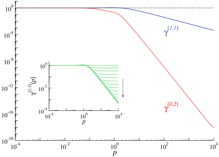
As an example of the numerical integration scheme that we have used we show in Fig. 1 the results for $\gamma^{(1,1)}(p)$ and $\gamma^{(0,2)}(p)$ for $d=3$ and $\varepsilon=2$. Both functions satisfy smoothly the renormalization condition at the infrared limit $p_{o}=10^{-4}$ while exhibiting a power-law decay in the ultra-violet. We observed the same qualitative behavior for any values of $d=2,3$ and $0\,<\,\varepsilon\,\leq\,4$. In the inset of Fig. 1 we show the regular convergence of the eddy diffusivity toward is final value.

We first discuss our numerical results in three dimensions.

\psfrag{LE}[b][b][1.2]{$\Lambda^{(\mathcal{E})}$}\psfrag{eps}[b][b][1.2]{$\varepsilon$}\includegraphics*[width=390.25534pt]{scaling-3d.eps}

Figure 3: (Color online) Scaling exponents $\Lambda$ in Eq. 99 of the dimensionless renormalized functions $\gamma^{(1,1)}(p)$ and $\gamma^{(0,2)}(p)$ and of the energy spectrum $\mathcal{E}$ as a function of $\varepsilon$ (blue solid circles) and $d=3$. We also show in red open squares the dependence of the scaling exponents $\eta_{\kappa}$ (upper panel) and $\eta_{F}$ (middle panel) on $\varepsilon$. The solid lines correspond to the respective renormalization group scaling of equations (77), and to $p^{-4\varepsilon/3}$ for the energy spectrum. The dashed lines in the upper and middle panels stand for the scalings $p^{-1}$ and $p^{1-d-4\varepsilon/3}$ respectively.

VI.1 3d

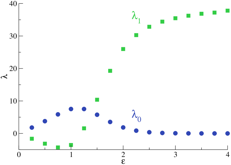
For each fixed value of $\varepsilon$ in $(0,4]$, we used the numerical scheme described above to integrate the equations (70) and obtained, for any initial value of the Grashof numbers for which we found convergence, a single stationary solution. This means that for each value of $\varepsilon$ there exist one single fixed point $(\lambda_{(0)},\lambda_{(1)})$ only. In Fig. 2, we show the dependence of the fixed point on $\varepsilon$. We have noted a slower convergence towards the solution as $\varepsilon\rightarrow 0$, making hard to explore the perturbative regime $\varepsilon\ll 1$. Nevertheless, our results suggest that the trivial fixed point of section IV.1 is reached in the limit of vanishing $\varepsilon$.

Surprisingly, for small values of $\varepsilon$, $\lambda_{(1)}<0$ and becomes positive for a value of $\varepsilon$ between $1$ and $1.25$. For $\varepsilon>2$, $\lambda_{(0)}$ decreases exponentially, but we always find a positive value.

To determine the ultra-violet scaling law as a function of $\varepsilon$, we computed

$$\Lambda^{(x,y)}\equiv\lim_{p\rightarrow\infty}\frac{\log\gamma^{(x,y)}}{\log p}\ ,$$ (99)

for $(x,y)=(1,1)$ or $(0,2)$, which defines the scaling exponent of the respective function. We denote with $\Lambda^{(\mathcal{E})}$ the analogous measure for the energy spectrum.

In Fig. 3 we show the scaling exponents $\eta_{\kappa}$ (red open squares in the upper panel) and $\eta_{F}$ (red open squares in the middle panel) as a function of $\varepsilon$. Our numerical results are in excellent agreement with the theoretical predictions (77) (solid lines), meaning that our closure yields the perturbative renormalization scaling. In the same figure we also show the scaling exponent of the dimensionless renormalized functions $\gamma^{(1.1)}$ (upper panel), $\gamma^{(0,2)}$ (middle panel) and of the energy spectrum (lower panel), as a function of $\varepsilon$.

Figure 4: (Color online) Basin of attraction of the fixed point in three dimensions, for different values of $\varepsilon$. Each yellow (light grey) dot, stands for an initial condition of $(\lambda_{(0)},\lambda_{(1)})$ for which convergence was reached. The square with dashed sides indicates the domain in which random initial conditions were drawn. The light grey solid circles stand for the trajectory of the fixed point in the $\lambda_{(0)}$-$\lambda_{(1)}$ plane and the blue (dark grey) circle, to the fixed point for the specific value of $\varepsilon$.

We observe two different regimes. In the first regime, for $\varepsilon<3/2$, the eddy diffusivity and the forcing amplitude scale in agreement with perturbative renormalization, as obtained in (78) and (79). Instead, for $\varepsilon>3/2$, both fields deviate individually from the perturbative renormalization prediction. In particular, in this regime the eddy diffusivity scales as $\gamma^{(1,1)}\sim p^{-1}$ independently of $\varepsilon$. This saturation has been predicted first in MoWe95 . More interestingly, the deviation of the forcing amplitude is such that the energy spectrum scaling is in agreement with perturbative renormalization i.e., $\mathcal{E}\sim p^{1-4\varepsilon/3}$, for all $\varepsilon$. Moreover, the deviations of the eddy diffusivity and the forcing amplitude from the perturbative renormalization coincide with those predicted by our simplified model, equations (91) and (96).

\psfrag{LE}[b][b][1.2]{$\Lambda^{(\mathcal{E})}$}\psfrag{eps}[b][b][1.2]{$\varepsilon$}\includegraphics*[width=390.25534pt]{scaling-3d-one-RC.eps}

Figure 5: (Color online) Scaling exponents $\Lambda$ in Eq. 99 of the dimensionless renormalized functions $\gamma_{\star}^{(1,1)}(p)$ and $\gamma_{\star}^{(0,2)}(p)$ and of the energy spectrum $\mathcal{E}$ as a function of $\varepsilon$ (blue solid circles) for the simplified model of section V and $d=3$. The red open squares in the upper panel correspond to $\eta_{\kappa}$. The solid and dashed lines correspond to the predicted scaling of equations (91), (96) and (97), for $\varepsilon<3/2$ and $\varepsilon>3/2$ respectively.

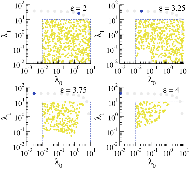
Finally, we would like to remark some properties of the convergence of the numerical scheme that we have used. As we mentioned above, the initial seed for the integration scheme comprises the initial value of the Grashof numbers. We have chosen this initial numbers by drawing $\lambda_{(0)}$ and $\lambda_{(1)}$ as random values in the domain $[0.01,10]$. By doing this, we found that the solution of our numerical scheme always converged to the fixed point when $\varepsilon<3$. However, for larger $\varepsilon$, we noticed that this was no longer the case. For $\varepsilon>3$ some of the initial conditions failed to converge. This can be seen in Fig. 4 in which we show as yellow (light grey) dots, those initial conditions that converged to the fixed point. We notice that the basin of attraction, limited to the $[0.01,10]\times[0.01,10]$ domain, shrinks as $\varepsilon$ grows. While we have no ultimate explanation for this behavior, it may be due either to the very small values that $\lambda_{(0)}$ attain for $\varepsilon>3$ or, more trivially, to the fact that our numerical scheme fails to converge to the fixed point (shown as the blue (dark grey) circle), when the initial condition is too far from it.

VI.2 Single renormalization condition

We have solved the simplified model of section V simply by setting $\eta_{F}=0$ and using the numerical scheme described above, by integrating equations (70), (76a) and (73a). In Fig. (5) we show the results that corroborate the predicted behavior of equations (91), (96) and (97).

In summary, we have obtained that the stationary solution to equations (70) is described by equations (91), (96) and (97), irrespectively if we impose the system to either one or two renormalization conditions.

Figure 6: (Color online) Dependence of the fixed point $(\lambda_{0},\lambda_{1})$ (blue dots) on $\varepsilon$ and $d=2$. The fixed point tends toward $(0,0)$ as $\varepsilon\rightarrow 0$.

VI.3 2d

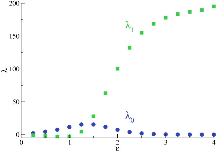
In two dimensions the results are in perfect agreement with the predictions of equations (91), (96) and (97), meaning that the fixed point found is consistent with the perturbative renormalization prediction. To start the discussion we show in Fig. 6 the fixed point for several values of $\varepsilon$. The behavior of the fixed point in two dimensions is qualitatively the same as in three dimensions, namely the fixed point $(\lambda_{0},\lambda_{1})$ tends to $(0,0)$ as $\varepsilon$ tends to zero; for $\varepsilon\lessapprox 1$, $\lambda_{(1)}<0$ and becomes positive for a value of $\varepsilon$ between $1$ and $1.25$; for $\varepsilon>2$, $\lambda_{(0)}$ decreases exponentially.

In Fig. 7 we show the scaling exponent $\eta_{\kappa}$ (red open squares in the upper panel) as a function of $\varepsilon$, in agreement with the prediction (77). Moreover, we also show the scaling exponent of the dimensionless renormalized functions $\gamma^{(1.1)}$ (upper panel), $\gamma^{(0,2)}$ (middle panel) and of the energy spectrum (lower panel), exhibiting the same behavior as in three dimensions, described by equations (91), (96) and (97).

Finally, as it was the case in three dimensions, in two dimensions we also observed that the basin of attraction shrinks for $\varepsilon\gtrapprox 3$, as is seen in Fig. 8.

\psfrag{LE}[b][b][1.2]{$\Lambda^{(\mathcal{E})}$}\psfrag{eps}[b][b][1.2]{$\varepsilon$}\includegraphics*[width=390.25534pt]{scaling-2d.eps}

Figure 7: (Color online) Scaling exponents $\Lambda$ in Eq. 99 of the dimensionless renormalized functions $\gamma^{(1,1)}(p)$ and $\gamma^{(0,2)}(p)$ and of the energy spectrum $\mathcal{E}$ as a function of $\varepsilon$ (blue solid circles) and $d=2$. We also show in red open squares the dependence of the scaling exponents $\eta_{\kappa}$ (upper panel) and $\eta_{F}$ (middle panel) on $\varepsilon$. The solid and dashed lines correspond to the predicted scaling of equations (91), (96) and (97), for $\varepsilon<3/2$ and $\varepsilon>3/2$ respectively.

VII Conclusions

Figure 8: (Color online) Basin of attraction of the fixed point in two dimensions, for different values of $\varepsilon$. Each yellow (light grey) dot, stands for an initial condition of $(\lambda_{(0)},\lambda_{(1)})$ for which convergence was reached. The square with dashed sides indicates the domain in which random initial conditions were drawn. The light grey solid circles stand for the trajectory of the fixed point in the $\lambda_{(0)}$-$\lambda_{(1)}$ plane and the blue (dark grey) circle, to the fixed point for the specific value of $\varepsilon$.

Power-law forcing provides us with a control parameter, $\varepsilon$, continuously changing the energy input from ultra-violet, as if due to thermal stirring, to infra-red as it is needed to interpret the stochastic Navier–Stokes as a model of fully developed Newtonian turbulence. The limit of vanishing $\varepsilon$ can be systematically investigated using the general principles of perturbative ultra-violet renormalization. These principles yield in three spatial dimensions the expression of the critical, fixed point, theory for vanishing $\varepsilon$. For fully developed turbulence the critical theory is not known, only some extrapolations can be made from the perturbative limit. The validity of these extrapolations is an open important question since they are based on the assumptions of the absence of any non-perturbative renormalization group fixed point and, provided this assumption holds, require controlling the limit of infinite integral scale of any statistical indicator of the theory after their perturbative expressions are re-summed for finite $\varepsilon$. The inquire of the Kraichnan model passive advection (see e.g. FaGaVe01 and references therein for review) has in recent years shed much light on how the limit of infinite integral scale can be investigated in a field theory model of fully developed turbulence. Namely, in the context of the Kraichnan model ultra-violet renormalization reduces to a trivial operation whilst the scaling properties of relevant physical indicators such as structure functions are fully specified by the analysis of composite operators (see e.g. AdAnVa98 and result discussion in KuMG07 ).

In this paper, we devise the simplest possible model of non-perturbative renormalization group flow complying with the requirements imposed by the general principles of ultra-violet renormalization as well as verifying the symmetries enjoyed by the stochastic Navier–Stokes equation. Specifically, these requirements translate in two classes of constraints. Vertices of the effective action must satisfy the Ward identities stemming from Galilean symmetry and space translational invariance. Furthermore, we adhere to the postulate of ultra-violet renormalization that no counter-term, can be consistently associated to non-local coupling. In other words, no independent renormalization constant can be associated either to the non-local forcing or to pressure. It is worth repeating here that explicit check show that non-local renormalization conditions yield inconsistencies already at second order in the perturbative expansion in powers of $\varepsilon$ (see e.g. AdHoKoVa05 ).

The intrinsic limitation of state-of-the art non-perturbative renormalization methods is that it allows us to derive explicit expressions only if we take into account a finite number of vertices in the renormalization group flow. As a guideline to operate this otherwise unjustified truncation, we restrict ourselves to interactions which can be assessed as relevant under renormalization at perturbative level. This is of course a dramatic approximation. We were encouraged in taking this step by the results, to some extent surprising, of CaChDeWs09 where it was shown that similar approximations appear to be able to capture the existence of a non-perturbative fixed point for the Kardar-Parisi-Zhang stochastic partial differential equation. This latter model shares with the stochastic Navier–Stokes equation invariance under Galilean transformations and convergence towards a non-Boltzmann steady state. An important difference between these two models resides, however, in the non-locality of the interactions that the incompressibility condition brings forth for Navier–Stokes. In our average action Ansatz (46) incompressibility simply appears in the form of transversal projectors acting on the classical field. In spite of this simple expression, the consequences of incompressibility are evident. The non-perturbative fixed point of the Kardar-Parisi-Zhang equation is suppressed. We also observe saturation to an $\varepsilon$-independent value of the scaling dimension of the eddy diffusivity at $\varepsilon=3/2$. Perturbative renormalization attributes to any integer power $n$ of the velocity field the scaling dimension $n\,(1-2\,\varepsilon/3)$. This means that the saturation we observe occurs exactly at the value of $\varepsilon$ when the velocity field (as well as all its integer powers) becomes an infra-red relevant operator. The fact may well be the indication of a change of critical behavior towards a regime not captured by our truncation. We do not observe saturation for $\varepsilon\,>\,2$ of the energy spectrum to the Kolmogorov value $-5/3$ for $d=3$, neither the inverse cascade $-5/3$ energy spectrum for $0\,<\,\varepsilon\,<\,2$ and $d=2$. If we identify the universality of the $-5/3$ energy spectrum in the above $\varepsilon$ domain with the presence of a scaling regime characterized by a constant energy flux, the inference is that it is not possible to describe a constant flux scaling regime in terms of an effective action comprising the vertices relevant under renormalization at perturbative level. Conversely, the average action Ansatz (46) yields scaling predictions in agreement with direct numerical simulations whenever the energy input at phenomenological level is not expected to sustain a constant flux solution of the Navier-Stokes equation ($0\,<\,\varepsilon\,<\,2$ for $d=3$ and $2\,<\,\varepsilon\,<\,3$ in $d=2$). Phenomenological reasoning suggests (see discussion in Frisch95 ; EyGo94 ) that the scaling properties of the constant flux solution are the consequence of the “localness” of the interactions within the turbulent fluid. This means that after isolating transport, “sweeping”, terms the critical theory should be described only by couplings involving local interactions in wave-number space. If this phenomenological reasoning is correct, constructing a renormalization group flow in the universality class of the constant flux solution poses a severe difficulty. On the one hand, our present results indicate that the flow should encompass in the Ansatz average action at least the set of proper vertices contributing to the flux. On the other, it is not a-priori evident how to reconcile these coupling with the requirement of localness.

As a conclusive remark we observe that renormalization methods may also have spin-offs for engineering applications. Obtaining, for example, a priori estimates for the eddy diffusivity and the Kolmogorov constant is very important for devising reliable large eddy simulations of turbulent flows Sagaut . In YaOr86 it was suggested that renormalized perturbation theory could be used to obtain quantitative predictions for the Kolmogorov constant. Whilst the treatment of the problem in YaOr86 can only be considered phenomenologically correct (see discussion in Ey94b and especially in section 2.10 of AdAnVa99 ), a controlled calculation of the Kolmogorov constant up to $O(\varepsilon^{3})$ in the renormalized perturbation theory evaluated for $\varepsilon=2$ in the limit of large spatial dimension can be found in AdAnGoKiKo08 . The result $C_{K}\sim 1.5+O(\varepsilon^{3},1/d)$ of AdAnGoKiKo08 is in reasonable agreement with experimental and numerical measurements Sre95 ; YeZh97 . The non-perturbative renormalization flow devised in this paper cannot be used in the present form to give predictions for indicators beyond scaling exponent. The reason is that the finite renormalization conditions we imposed only fix the ratio $F_{o}/\kappa^{3}$ between the “bare” parameters of the stochastic Navier–Stokes equation. In other words, we did not specify (neither had the need of specifying) the units in which the energy input is measured. Such way of proceeding is perfectly in line with the general renormalization group ideology which aims at determining scaling exponents as only indicators of universality classes. It is possible, however, to envisage imposing different renormalization conditions fully specifying the values of the “bare” parameters $F_{o}$, and $\kappa$. This is an issue which we leave for future work.

VIII Acknowledgments

We are grateful to Luca Peliti for pointing out to us references LiFi86 ; LiFi87 and their potential relevance for a renormalization group theory for the $2d$ inverse cascade. The work PMG was supported by Finnish Academy CoE “Analysis and Dynamics” and from the KITP program “The nature of Turbulence” (grant No. NSF PHY05-51164). The authors acknowledge support from the ESF and hospitality of NORDITA where part of this work has been done during their stay within the framework of the ”Non-equilibrium Statistical Mechanics” program.

Appendix A Variations of the generating of function

A.1 Renormalization group flow

Let us consider the deformation of (1) induced by the replacements $\kappa\mapsto\kappa+\kappa_{m_{r}}R$ and $\boldsymbol{f}\mapsto\boldsymbol{f}^{\prime}+\bar{\boldsymbol{\jmath}}$. We suppose that $\boldsymbol{f}^{\prime}$ is obtained from applying to $\boldsymbol{f}$ an high pass filter with infra-red cut off $m_{r}$. We have then

$$m_{r}\partial_{m_{r}}\mathcal{Z}_{\left(\boldsymbol{\jmath},\bar{\boldsymbol{\jmath}}\right)}=\prec\,e^{\boldsymbol{\jmath}\star\boldsymbol{v}}\boldsymbol{\jmath}\star(m_{r}\partial_{m_{r}}\boldsymbol{v})\,\succ\ ,$$ (100)

with

$$m_{r}\partial_{m_{r}}\boldsymbol{v}(\boldsymbol{x},t;\bar{\boldsymbol{\jmath}}+\boldsymbol{f})=\frac{\delta\boldsymbol{v}(\boldsymbol{x},t;\bar{\boldsymbol{\jmath}}+\boldsymbol{f})}{\delta\bar{\boldsymbol{\jmath}}}\star$$ (101)

$$\left\{(m_{r}\partial_{m_{r}}\kappa_{m_{r}}\,R)\star\partial^{2}\boldsymbol{v}+(m_{r}\partial_{m_{r}}\boldsymbol{f}^{\prime})\right\}\ .$$

In (101) the fluctuating response function satisfies

$$\frac{\delta\boldsymbol{v}(\boldsymbol{x}_{1},t_{1})}{\delta\bar{\boldsymbol{\jmath}}(\boldsymbol{x}_{2},t_{2})}=0\hskip 14.22636pt\forall\,t_{2}\leq t_{1}\ .$$ (102)

We furthermore interpret the product of the time $\delta$-correlated Gaussian field $\boldsymbol{f}^{\prime}$ with other functionals in (100) according to Stratonovich convention in order to preserve ordinary calculus. Using (102) we can write

$$\prec\,e^{\boldsymbol{\jmath}\star\boldsymbol{v}}\frac{\delta(\boldsymbol{\jmath}\star\boldsymbol{v})}{\delta\bar{\boldsymbol{\jmath}}}\star(m_{r}\partial_{m_{r}}\kappa_{m_{r}}\,R)\star\partial^{2}\boldsymbol{v}\,\succ$$ (103)

$$=\prec\,\frac{\delta\,e^{\boldsymbol{\jmath}\star\boldsymbol{v}}}{\delta\bar{\boldsymbol{\jmath}}}\star(m_{r}\partial_{m_{r}}\kappa_{m_{r}}\,R)\star\partial^{2}\boldsymbol{v}\,\succ$$

$$=\mathrm{tr}(m_{r}\partial_{m_{r}}\kappa_{m_{r}}\,R)\star\partial^{2}\mathcal{Z}_{(\boldsymbol{\jmath},\bar{\boldsymbol{\jmath}})}^{(1,1)}\ .$$

Furthermore, a functional integration by parts yields

$$\prec\,e^{\boldsymbol{\jmath}\star\boldsymbol{v}}\frac{\delta(\boldsymbol{\jmath}\star\boldsymbol{v})}{\delta\bar{\boldsymbol{\jmath}}}\star(m_{r}\partial_{m_{r}}\,\boldsymbol{f}^{\prime})\,\succ$$ (104)

$$=\frac{1}{2}\prec\,(m_{r}\partial_{m_{r}}\,\mathsf{F}^{\prime})\star\,\frac{\delta^{2}\,e^{\boldsymbol{\jmath}\star\boldsymbol{v}}}{\delta\bar{\boldsymbol{\jmath}}\delta\bar{\boldsymbol{\jmath}}}\succ\ ,$$

the factor $1/2$ being a consequence of Stratonovich convention.

A.2 Ward identity

Let $\boldsymbol{r}_{t}:\mathbb{R}\to\mathbb{R}^{d}$ a smooth path. The generalized Galilean transformation

$$\tilde{\boldsymbol{x}}=\boldsymbol{x}+\varepsilon\,\boldsymbol{r}_{t}\ ,$$ (105a)

$$\tilde{\boldsymbol{v}}=\boldsymbol{v}+\varepsilon\,\dot{\boldsymbol{r}}_{t}\ ,$$ (105b)

leaves (1) invariant in form when if accompanied by the redefinition of the forcing $\tilde{\boldsymbol{f}}=\boldsymbol{f}+\varepsilon\,\ddot{\boldsymbol{r}}_{t}$. We must have therefore

$$\mathcal{Z}_{(\boldsymbol{\jmath},\bar{\boldsymbol{\jmath}})}^{(\varepsilon)}=\mathcal{Z}_{(\boldsymbol{\jmath},\bar{\boldsymbol{\jmath}})}\ .$$ (106)

When we differentiate this equality at $\varepsilon$ equal zero and use (101) we obtain after standard manipulations (see e.g. Zinn )

$$0=\ddot{\boldsymbol{r}}\star\left(\frac{\delta\,\mathcal{W}_{\left(\boldsymbol{\jmath},\bar{\boldsymbol{\jmath}}\right)}}{\delta\boldsymbol{\bar{\jmath}}}\right)+$$ (107)

$$\boldsymbol{\jmath}\star\left(\boldsymbol{r}\cdot\boldsymbol{\partial}\frac{\delta\,\mathcal{W}_{\left(\boldsymbol{\jmath},\bar{\boldsymbol{\jmath}}\right)}}{\delta\boldsymbol{\jmath}}-\dot{\boldsymbol{r}}\right)+\boldsymbol{\bar{\jmath}}\star\,\left(\boldsymbol{r}\cdot\boldsymbol{\partial}\frac{\delta\,\mathcal{W}_{\left(\boldsymbol{\jmath},\bar{\boldsymbol{\jmath}}\right)}}{\delta\boldsymbol{\bar{\jmath}}}\right)\ .$$

An alternative way to derive the results of this appendix is based on the Janssen–De Dominicis De76 ; Ja76 path integral representation of (23). We refer to CoTo97 for a detailed presentation.

Appendix B Janssen–De Dominicis path integral and optimal fluctuation

The Janssen–De Dominicis De76 ; Ja76 representation is the formal measure on path space obtained by requiring through an infinite dimensional product of Dirac $\delta$-functions that at any space-time point (1) be satisfied. The resulting expression is then averaged over the realizations of the stochastic forcing. We obtain

$$\mathcal{Z}_{(\boldsymbol{\jmath},\bar{\boldsymbol{\jmath}})}=\int D[\boldsymbol{v}]D[\bar{\boldsymbol{v}}]e^{-\mathcal{A}}\ ,$$ (108a)

$$\mathcal{A}=\frac{\bar{\boldsymbol{v}}\star\mathsf{F}\star\bar{\boldsymbol{v}}}{2}-\boldsymbol{\jmath}\star\boldsymbol{v}$$ (108b)

$$-\imath\bar{\boldsymbol{v}}\star[(\partial_{t}-\kappa\partial_{\boldsymbol{x}}^{2})\boldsymbol{v}+\mathsf{T}(\boldsymbol{v}\cdot\partial_{\boldsymbol{x}}\boldsymbol{v})-\bar{\boldsymbol{\jmath}}]\ .$$

A precise meaning to (108) can be given on a space-time lattice using a pre-point discretization $dt\,(\bar{\boldsymbol{v}}\cdot\partial_{t}\boldsymbol{v})\sim\bar{\boldsymbol{v}}(t_{i})\cdot[\boldsymbol{v}(t_{i+1})-\boldsymbol{v}(t_{i})]$, $dt\,f(\bar{\boldsymbol{v}}(t),\boldsymbol{v}(t))\sim dt\,f(\bar{\boldsymbol{v}}(t_{i}),\boldsymbol{v}(t_{i}))$ for all other terms in (108b). Notice that in the limit of vanishing stirring $\mathsf{F}\downarrow 0$, (108) recovers the Fourier representation of a product of Dirac $\delta$-functions localizing the measure over the deterministic decaying dynamics. In this sense (108) remains meaningful also as a formal measure inclusive of compressible fluctuations. ¿From (108b) a stationary phase approximation yields the weak noise limit of the free energy $\mathcal{W}_{(\boldsymbol{\jmath},\bar{\boldsymbol{\jmath}})}$ around an optimal fluctuation $\boldsymbol{v}^{*}$. As usual Erdelyi , the stationary phase condition is derived by closing a contour in the complex variables

$$\bar{\boldsymbol{v}}=\bar{\boldsymbol{v}}_{\Re}+\imath\bar{\boldsymbol{v}}_{\Im}\ ,$$ (109)

which decomposes (108b) into the real and imaginary parts

$$\Re\mathcal{A}_{(\boldsymbol{\jmath},\bar{\boldsymbol{\jmath}})}=\frac{\bar{\boldsymbol{v}}_{\Re}\star\mathsf{F}\star\bar{\boldsymbol{v}}_{\Re}}{2}-\boldsymbol{\jmath}\star\boldsymbol{v}+$$ (110a)

$$\bar{\boldsymbol{v}}_{\Im}\star\left\{(\partial_{t}-\kappa\partial_{\boldsymbol{x}}^{2})\boldsymbol{v}+\mathsf{T}(\boldsymbol{v}\cdot\partial_{\boldsymbol{x}}\boldsymbol{v})-\frac{1}{2}\mathsf{F}\star\bar{\boldsymbol{v}}_{\Im}-\bar{\boldsymbol{\jmath}}\right\}\ ,$$

$$\Im\mathcal{A}_{(\boldsymbol{\jmath},\bar{\boldsymbol{\jmath}})}=$$ (110b)

$$-\bar{\boldsymbol{v}}_{\Re}\star\left\{(\partial_{t}-\kappa\partial_{\boldsymbol{x}}^{2})\boldsymbol{v}+\mathsf{T}(\boldsymbol{v}\cdot\partial_{\boldsymbol{x}}\boldsymbol{v})-\mathsf{F}\star\bar{\boldsymbol{v}}_{\Im}-\bar{\boldsymbol{\jmath}}\right\}\ .$$

The stationary phase condition $\Im\mathcal{A}_{(\boldsymbol{\jmath},\bar{\boldsymbol{\jmath}})}=0$ can then be solved for $\bar{\boldsymbol{v}}_{\Im}$ and leaves with a convex functional of the principal field $\boldsymbol{v}$. Assuming that we can minimize such functional for some assigned boundary condition, we find within logarithmic accuracy

$$\mathcal{W}_{(\boldsymbol{\jmath},\bar{\boldsymbol{j}})}\sim\boldsymbol{\jmath}\star\boldsymbol{v}^{*}$$ (111)

$$-\frac{\parallel(\partial_{t}-\kappa\partial_{\boldsymbol{x}}^{2})\boldsymbol{v}^{*}+\mathsf{T}(\boldsymbol{v}\cdot\partial_{\boldsymbol{x}}\boldsymbol{v})^{*}-\bar{\boldsymbol{\jmath}}\parallel_{\mathsf{F}}^{2}}{2}\,$$

where $\parallel\boldsymbol{v}\parallel_{\mathsf{F}}^{2}$ stands for $\parallel\boldsymbol{v}\parallel_{\mathsf{F}}^{2}=\boldsymbol{v}\star\mathsf{F}^{-1}\star\boldsymbol{v}$. The Legendre transform gives the conditions

$$\boldsymbol{u}=\boldsymbol{v}^{*}\ ,$$ (112a)

$$\bar{\boldsymbol{u}}=\mathsf{T}\star\mathsf{F}^{-1}\star\left\{(\partial_{t}-\kappa\partial_{\boldsymbol{x}}^{2})\boldsymbol{v}^{*}+\mathsf{T}(\boldsymbol{v}\cdot\partial_{\boldsymbol{x}}\boldsymbol{v})^{*}-\bar{\boldsymbol{\jmath}}\right\}$$ (112b)

whence we finally obtain (29). It must be stressed here that the “measure” $D[\boldsymbol{v}]D[\bar{\boldsymbol{v}}]$ in (108) does not exist in any rigorous mathematical sense. Thus, the above calculation is only formal. We give it a meaning in the following sense. A Gaussian measure is fully specified by its first and second moments. Since $\mathsf{F}$ is an incompressible correlation function it is consistent to consider the fields $\bar{\boldsymbol{v}},\bar{\boldsymbol{\jmath}}$ incompressible by definition. The field $\boldsymbol{v}^{*}$ is also incompressible because is solution of the classical Navier–Stokes equation with vanishing initial condition at time $t=-\infty$ and sustained by an incompressible forcing. Finally, the inversion operation in (112b) makes sense only away from the kernel of the transverse correlation $\mathsf{F}$ which therefore implies that $\bar{\boldsymbol{u}}$ is also incompressible.

Appendix C Explicit expression of the convolutions

An alternative derivation of the renormalization group equations is obtained if we observe that we may interpret the free energy defined by the Ansatz for the average action (62) as solution of a formal Janssen-De Dominicis De76 ; Ja76 path integral

$$\mathcal{W}(\boldsymbol{\jmath}\,,\boldsymbol{\bar{\jmath}})=\lim_{\varepsilon\searrow 0}\varepsilon\,\ln\int D[\boldsymbol{u}]D[\boldsymbol{\bar{u}}]\,e^{\frac{\boldsymbol{\jmath}\star\boldsymbol{u}+\boldsymbol{\bar{\jmath}}\star\boldsymbol{\bar{u}}-\mathcal{U}(\boldsymbol{u}\,,\boldsymbol{\bar{u}})}{\varepsilon}}\ .$$ (113)

Computing the right hand side in a perturbative expansion in powers of the interaction vertex (51),(55) we obtain by standard diagrammatic techniques

$$\kappa_{m_{r}}\,p^{2}\,\gamma^{(1,1)}(p/m_{r})=$$ (114)

$$\int\frac{d^{d}k}{(2\,\pi)^{d}}\frac{\left(1-\phi^{2}\right)\,N^{(1,1)}(p,k,\phi)\,g^{(0,2)}(k)}{2\,g^{(1,1)}(k)\,D_{1}(p,k,\phi)}\ ,$$

and

$$[\lambda_{(0)}m_{r}^{2-d-2\,\varepsilon}+\lambda_{(1)}]p^{2}\gamma^{(0,2)}(p/m_{r})=$$ (115)

$$\int\frac{d^{d}k}{(2\,\pi)^{d}}\frac{\left(1-\phi^{2}\right)\,N^{(0,2)}(p,k,\phi)\,\,g^{(0,2)}(Q)\,g^{(0,2)}(k)}{4\,g^{(1,1)}(k)\,g^{(1,1)}(Q)\,D_{1}(p,k,\phi)}\ .$$

We recover equations (70) by taking the logarithmic derivative $m_{r}\partial_{m_{r}}$ of both sides of (114), (115) Note that in (114), (115) we denoted

$$\boldsymbol{Q}:=\boldsymbol{p}-\boldsymbol{k}\ ,$$ (116)

and $\phi$ the cosine between the external $\boldsymbol{p}$ and the integration $\boldsymbol{k}$ wave-numbers:

$$\phi:=\frac{\boldsymbol{p}\cdot\boldsymbol{k}}{p\,k}\ .$$ (117)

We also defined the auxiliary integrand factors

$$D_{1}(p,k,\phi)=k^{2}\,g^{(1,1)}(k)+Q^{2}\,g^{(1,1)}(Q)\ ,$$ (118)

$$D_{2}(p,k,\phi)=2\,k^{2}\,g^{(1,1)}(k)+Q^{2}\,g^{(1,1)}(Q)\ ,$$ (119)

and the constants

$$C_{d}^{-1}=(d-1)\,\int_{-1}^{1}d\phi\,(1-\phi^{2})^{\frac{d-3}{2}}\ .$$ (120)

Finally, the convolutions depends upon certain integral kernels which stem from the expansion up to one loop accuracy of the Ansatz average action (62). These are

$$N^{(1,1)}(p,k,\phi):=$$ (121a)

$$\frac{(d-1)\,p^{3}\,(p-2\,\phi\,k)+k^{2}\,p\,[(d-3)\,p+2\,\phi\,k]}{k^{2}\,(p^{2}+k^{2}-2\,k\,p\,\phi)}\ ,$$

$$\tilde{N}^{(1,1)}(p,k,\phi):=$$ (121b)

$$\frac{p\,k\,[(d-1)\,p\,k-2\,(p^{2}+k^{2}-2\,p\,k\,\phi)\,\phi]}{k^{2}\,(p^{2}+k^{2}-2\,k\,p\,\phi)}\ ,$$

for the eddy diffusivity vertex, (121b) will be needed below, and

$$N^{(0,2)}(p,k,\phi):=$$ (122)

$$\frac{p^{2}\,[(d-1)\,p^{2}-2\,d\,p\,k\,\phi+2\,k^{2}\left(d+2\,\phi^{2}-2\right)]}{k^{2}\,(p^{2}+k^{2}-2\,k\,p\,\phi)^{2}}\ ,$$

for the force vertex. Finally in (70) there appear terms of the form

$$G^{(i,j)}_{l}(p):=$$ (123)

$$\frac{C_{d}}{2\,p^{2}}\int_{0}^{\infty}\frac{dk}{k}\,k^{d}\int_{-1}^{1}d\phi\,(1-\phi^{2})^{\frac{d-1}{2}}\,V^{(i,j)}_{l}(p,k,\phi)\ ,$$

with $l$ taking values $\left\{F,\kappa,o\right\}$ and $V^{(i,j)}_{l}(p,k,\phi)$ the non-linear convolutions specified below.

C.1 Equation for the eddy diffusivity vertex

The following three non-linear convolutions enter (70a):

$$V^{(1,1)}_{F}(p,k,\phi):=\frac{N^{(1,1)}(p,k,\phi)\,\lambda_{(1)}\chi_{(1)}(k)}{g^{(1,1)}(k)\,D_{1}(p,k,\phi)}\ ,$$ (124)

with coefficient $\eta_{F}$,

$$V^{(1,1)}_{\kappa}(p,k,\phi):=\frac{\check{R}(k)}{[D_{1}(p,k,\phi)]^{2}}\times$$ (125)

$$\left\{\frac{D_{2}(p,k,\phi)\,N^{(1,1)}(p,k,\phi)\,g^{(0,2)}(k)}{[g^{(1,1)}(k)]^{2}}\right.$$

$$\left.+\frac{k^{4}\,\tilde{N}^{(1,1)}(p,k,\phi)\,g^{(0,2)}(Q)}{Q^{2}g^{(1,1)}(Q)}\right\}\ ,$$

with coefficient $\eta_{\kappa}$, and

$$V^{(1,1)}_{o}(p,k,\phi)=$$ (126)

$$\frac{N^{(1,1)}(p,k,\phi)\,\sum_{i=0}^{1}\lambda_{(i)}\,(\boldsymbol{k}\cdot\partial_{\boldsymbol{k}}-d_{F_{(i)}})\chi_{(i)}(k)}{g^{(1,1)}(k)\,D_{1}(p,k,\phi)}$$

$$-\frac{(\boldsymbol{k}\cdot\partial_{\boldsymbol{k}}\check{R})(k)}{[D_{1}(p,k,\phi)]^{2}}\left[\frac{D_{2}(p,k,\phi)\,N^{(1,1)}(p,k,\phi)\,g^{(0,2)}(k)}{g^{(1,1)}(k)}\right.$$

$$\left.+\frac{k^{4}\,\tilde{N}^{(1,1)}(p,k,\phi)\,g^{(0,2)}(Q)}{Q^{2}\,g^{(1,1)}(Q)}\right]\ ,$$

with coefficient equal to the unity.

C.2 Equation for the force vertex

The following three non-linear convolutions enter (70b):

$$V_{F}^{(0,2)}(p,k,\phi):=\frac{N^{(0,2)}(p,k,\phi)\,g^{(0,2)}(Q)\,\chi_{(1)}(k)}{g^{(1,1)}(Q)\,g^{(1,1)}(k)\,D_{1}(p,k,\phi)}\ ,$$ (127)

with coefficient $\eta_{F}$,

$$V_{\kappa}^{(0,2)}(p,k,\phi):=N^{(0,2)}(p,k,\phi)\times$$ (128)

$$\frac{g^{(0,2)}(Q)\,g^{(0,2)}(k)\,\check{R}(k)D_{2}(p,k,\phi)}{g^{(1,1)}(Q)\,[g^{(1,1)}(k)]^{2}[D_{1}(p,k,\phi)]^{2}}\ ,$$

with coefficient $\eta_{\kappa}$, and

$$V_{o}^{(0,2)}(p,k,\phi):=\frac{N^{(0,2)}(p,k,\phi)\,g^{(0,2)}(Q)}{g^{(1,1)}(Q)\,g^{(1,1)}(k)\,D_{1}(p,k,\phi)}\times$$ (129)

$$\left\{\sum_{i=0}^{1}\lambda_{(i)}\left(\boldsymbol{k}\cdot\partial_{\boldsymbol{k}}-d_{F_{(i)}}\right)\chi_{(i)}(k,\mu)\right.$$

$$\left.-\frac{(\boldsymbol{k}\cdot\partial_{\boldsymbol{k}}\check{R})(k)\,g^{(0,2)}(k)}{g^{(1,1)}(k)}\,\frac{D_{2}(p,k,\phi)}{D_{1}(p,k,\phi)}\right\}\ ,$$

with coefficient equal to the unity.

References

- (1) A. N. Kolmogorov, Akademiia Nauk SSSR Doklady 30, 301 (1941).
- (2) A. N. Kolmogorov, Royal Society of London Proceedings Series A 434, 15 (1991).
- (3) U. Frisch, Turbulence: the legacy of AN Kolmogorov (Cambridge University Press, 1995).
- (4) D. Bernard, Physical Review E 60, 6184 (1999), chao-dyn/9902010.
- (5) D. Bernard, Europhysics Letters 50, 333 (2000), chao-dyn/9904034.
- (6) E. Lindborg, Journal of Fluid Mechanics 326, 343 (1996).
- (7) R. H. Kraichnan, Physics of Fluids 10, 1417 (1967).
- (8) G. Boffetta, Journal of Fluid Mechanics 589, 253 (2007), nlin/0612035.
- (9) K. Nam, T. M. Antonsen, P. N. Guzdar, and E. Ott, Physical Review Letters 83, 3426 (1999).
- (10) P. Constantin and F. Ramos, Communications in Mathematical Physics 275, 529 (2007), math/0611782.
- (11) G. Falkovich, Fluid Mechanics: A Short Course for Physicists (Cambridge University Press, 2011).
- (12) D. Forster, D. R. Nelson, and M. J. Stephen, Physical Review Letters 36, 867 (1976).
- (13) D. Forster, D. R. Nelson, and M. J. Stephen, Physical Review A 16, 732 (1977).
- (14) C. De Dominicis and P. C. Martin, Physical Review A 19, 419 (1979).
- (15) J. Zinn-Justin, Quantum field theory and critical phenomena, 4th ed. (Oxford University Press, 2002).
- (16) J. L. Cardy, Scaling and renormalization in statistical physics, Cambridge lecture notes in physics Vol. 5 (Cambridge University Press., 1996).
- (17) L. T. Adzhemyan, N. V. Antonov, and A. N. Vasil’ev, The field theoretic renormalization group in fully developed turbulence (Gordon and Breach, 1999).
- (18) J.-D. Fournier and U. Frisch, Physical Review A 28, 1000 (1983).
- (19) A. Sain, Manu, and R. Pandit, Physical Review Letters 81, 4377 (1998).
- (20) L. Biferale, M. Cencini, A. S. Lanotte, M. Sbragaglia, and F. Toschi, New Journal of Physics 6, 37 (2004), nlin/0401020.
- (21) A. Mazzino, P. Muratore-Ginanneschi, and S. Musacchio, Physical Review Letters 99, 144502 (2007), 0907.3396.
- (22) A. Mazzino, P. Muratore-Ginanneschi, and S. Musacchio, Journal of Statistical Mechanics: Theory and Experiment 2009, 10012 (2009), 0907.3396.
- (23) J. Honkonen, Physical Review E 58, 4532 (1998).
- (24) R. Lipowsky and M. E. Fisher, Physical Review Letters 57, 2411 (1986).
- (25) R. Lipowsky and M. E. Fisher, Physical Review B 36, 2126 (1987).
- (26) L. Canet, H. Chaté, B. Delamotte, and N. Wschebor, Physical Review Letters 104, 150601 (2009), 0905.1025.
- (27) J. Berges, N. Tetradis, and C. Wetterich, Physics Reports 363, 223 (2002), hep-ph/0005122.
- (28) C. Bagnuls and C. Bervillier, Physics Reports 348, 91 (2001), hep-th/0002034.
- (29) L. Canet and H. Chaté, Journal of Physics A Mathematical General 40, 1937 (2007), cond-mat/0610468.
- (30) C.-Y. Mou and P. B. Weichman, Physical Review E 52, 3738 (1995).
- (31) J. C. Bowman, J. A. Krommes, and M. Ottaviani, Physics of Plasmas 5, 3558 (1993).
- (32) S. D. Głazek and K. G. Wilson, Physical Review B 69, 094304 (2004), cond-mat/0303297.
- (33) A. Kupiainen, Séminaire Bourbaki 62, 1016 (2009-2010), 1005.0587.
- (34) C. Wetterich, Nuclear Physics B 352, 529 (1991).
- (35) J. Polchinski, Nuclear Physics B 231, 269 (1984).
- (36) C. Wetterich, Physics Letters B 301, 90 (1993).
- (37) J. Honkonen and M. Y. Nalimov, Zeitschrift für Physik B Condensed Matter 99, 297 (1996).
- (38) L. T. Adzhemyan, J. Honkonen, M. V. Kompaniets, and A. N. Vasil’ev, Physical Review E 71, 036305 (2005), nlin/0407067.
- (39) M. Bonini, M. D’Attanasio, and G. Marchesini, Nuclear Physics B 418, 81 (1994), hep-th/9307174.
- (40) E. Frey and U. C. Täuber, Physical Review E 50, 1024 (1994), cond-mat/9406068.
- (41) P. Tomassini, Physics Letters B 411, 117 (1997).
- (42) R. Collina and P. Tomassini, On the ERG approach in well developed turbulence, hep-th/9709185, 1997.
- (43) G. Falkovich, K. Gawȩdzki, and M. Vergassola, Reviews of Modern Physics 73, 913 (2001), cond-mat/0105199.
- (44) L. T. Adzhemyan, N. V. Antonov, and A. N. Vasil’ev, Physical Review E 58, 1823 (1998), chao-dyn/9801033.
- (45) A. Kupiainen and P. Muratore-Ginanneschi, Journal of Statistical Physics 126, 669 (2007), nlin/0603031.
- (46) G. L. Eyink and N. Goldenfeld, Physical Review E 50, 4679 (1994), cond-mat/9407021.
- (47) P. Sagaut, Large Eddy Simulation for Incompressible Flows, 3rd ed. (Springer, 2006).
- (48) V. Yakhot and S. A. Orszag, Journal of Scientific Computing 1, 3 (1986).
- (49) G. L. Eyink, Physics of Fluids 6, 3063 (1994).
- (50) L. T. Adzhemyan, N. V. Antonov, P. B. Gol’din, T. L. Kim, and M. V. Kompaniets, Journal of Physics A: Mathematical and Theoretical 41, 495002 (2008), 0809.1289.
- (51) K. R. Sreenivasan, Physics of Fluids 7, 2778 (1995).
- (52) P. K. Yeung and Y. Zhou, Physical Review E 56, 1746 (1997).
- (53) C. De Dominicis, Journal de Physique Colloques 37, C1 (1976).
- (54) H.-K. Janssen, Zeitschrift für Physik B Condensed Matter 23, 377 (1976).
- (55) A. Erdélyi, Asymptotic expansionsDover books on advanced mathematics (Courier Dover Publications, 1956).