THERMAL PRODUCTION OF AXINO DARK MATTER

Abstract

We discuss certain features of the low energy effective interactions of axion supermultiplet, which are relevant for axino cosmology, and examine the implication to thermal production of axino in the early Universe.

PACS numbers:

1 Introduction

Supersymmetric and axionic extension of the standard model provides an appealing solution to both of the gauge hierarchy problem and the strong CP problem. In such model, the superpartners of axion, i.e. the axino and saxion, can have a variety of cosmological implications[1, 2]. In particular, axino can be a good candidate for cold dark matter, depending upon the mechanism of supersymmetry breaking and cosmological evolution in the early Universe. Even when axino is not stable, so does not constitute the dark matter, it can affect the evolution of early Universe in various ways. For instance, late decays of axino might affect the relic dark matter density and/or the Big-Bang nucleosynthesis and/or the large scale structure formation[3].

One of the key issues in axino cosmology is the thermal production of axino by scattering or decay of particles in thermal equilibrium in the early Universe[4]. Most of the previous analysis of thermal axino production[4] is based on the local effective interaction of the form

$$\int d^{2}\theta\,\frac{1}{32\pi^{2}}\frac{A}{v_{PQ}}W^{a\alpha}W^{a}_{\alpha},$$ (1)

where $v_{PQ}$ is the scale of spontaneous breakdown of the PQ symmetry, and $A=(s+ia)/\sqrt{2}+\sqrt{2}\theta\tilde{a}+\theta^{2}F^{A}$ is the axion superfield which contains the axion $a$, the saxion $s$, and the axino $\tilde{a}$ as its component fields. In some cases, for instance the KSVZ-type model with heavy quark supermultiplet having a mass $M_{Q}\sim v_{PQ}$, the effective interaction (1) provides a good description of the low energy dynamics of axion supermultiplet. However, in other cases, e.g. the KSVZ-type model with $M_{Q}\ll v_{PQ}$ or the DFSZ-type model without exotic heavy quark, analysis using the effective interaction (1) alone yields a highly overestimated axino production rate as the correct rate experiences a cancellation due to other effective interactions[5]. In this talk, we discuss first generic structure of the low energy effective interactions of axion supermultiplet in models having a UV completion in which the PQ symmetry is linearly realized, and then consider its implication to cosmological axino production.

2 Effective interactions of axion supermultiplet

Generic Wilsonian effective lagrangian of the axion superfield at energy scale $\Lambda$ below the PQ scale $v_{PQ}$ takes the form

$${\cal L}_{\rm eff}(\Lambda) = \int d^{4}\theta\,\left(K_{A}(A+A^{\dagger})+Z_{n}(A+A^{\dagger})\Phi_{n}^{\dagger}\Phi_{n}\right)$$ (2)

$$+ \left[\,\int d^{2}\theta\,\left(\frac{1}{4}f^{\rm eff}_{a}(A)W^{a\alpha}W^{a}_{\alpha}+W_{\rm eff}\right)+{\rm h.c}\,\right],$$

where $\{\Phi_{n}\}$ denote the light gauge-charged matter fields, and

$$K_{A} = \frac{1}{2}(A+A^{\dagger})^{2}+{\cal O}\left(\frac{(A+A^{\dagger})^{3}}{v_{PQ}}\right),$$

$$\ln Z_{n} = \left.\ln Z_{n}\right|_{A=0}+\tilde{y}_{n}\frac{(A+A^{\dagger})}{v_{PQ}}+{\cal O}\left(\frac{(A+A^{\dagger})^{2}}{v^{2}_{PQ}}\right),$$

$$f^{\rm eff}_{a} = \frac{1}{\hat{g}_{a}^{2}(\Lambda)}-\frac{C^{a}_{W}}{8\pi^{2}}\frac{A}{v_{PQ}},$$

$$W_{\rm eff} = \frac{1}{2}e^{-(\tilde{x}_{n}+\tilde{x}_{m})A/v_{PQ}}M_{mn}\Phi_{m}\Phi_{n}$$

$$+ \frac{1}{6}e^{-(\tilde{x}_{n}+\tilde{x}_{m}+\tilde{x}_{p})A/v_{PQ}}\lambda_{mnp}\Phi_{m}\Phi_{n}\Phi_{p}.$$

The PQ symmetry is realized as $U(1)_{PQ}:A\rightarrow A+i\alpha v_{PQ},\Phi_{n}\rightarrow e^{i\tilde{x}_{n}\alpha}\Phi_{n}$, and the Wilsonian couplings between the axion superfield and the gauge/matter superfields are given by

$$\Delta_{1}{\cal L}(\Lambda) = -\int d^{2}\theta\,\frac{C^{a}_{W}}{32\pi^{2}}\frac{A}{v_{PQ}}W^{a\alpha}W^{a}_{\alpha},$$

$$\Delta_{2}{\cal L}(\Lambda) = \int d^{4}\theta\,\,\tilde{y}_{n}\frac{(A+A^{\dagger})}{v_{PQ}}\Phi_{n}^{\dagger}\Phi_{n},$$

$$\Delta_{3}{\cal L}(\Lambda) = -\int d^{2}\theta\,\frac{A}{v_{PQ}}\Big{[}\,\frac{(\tilde{x}_{m}+\tilde{x}_{n})}{2}M_{mn}\Phi_{n}\Phi_{m}$$ (3)

$$\qquad+\,\frac{(\tilde{x}_{m}+\tilde{x}_{n}+\tilde{x}_{p})\lambda_{mnp}}{6}\Phi_{m}\Phi_{n}\Phi_{p}\,\Big{]}.$$

Then there are three quantities $\{\,C_{W}^{a},\,C^{a}_{PQ},\,C^{a}_{1PI}\,\}$ which are related to the axino coupling to gauge supermultiplets, where $C_{W}^{a}$ are the Wilsonian couplings in (2), $C^{a}_{PQ}$ are the PQ anomaly coefficients defined as

$$\partial_{\mu}J^{\mu}_{PQ}=\frac{g^{2}}{16\pi^{2}}C_{PQ}^{a}F^{a\mu\nu}\tilde{F}^{a}_{\mu\nu},$$ (4)

and finally $C_{1PI}^{a}$ determines the leading part of the 1PI axino-gaugino-gauge boson amplitude

$${\cal A}^{a}_{1PI}(k,q,p)=-\frac{g^{2}}{16\pi^{2}\sqrt{2}v_{PQ}}\tilde{C}^{a}_{1PI}\delta^{4}(k+q+p)\bar{u}(k)\sigma_{\mu\nu}\gamma_{5}v(q)\epsilon^{\mu}p^{\nu}$$ (5)

which shows the behavior

$$\tilde{C}_{1PI}^{a}(k^{2}=q^{2}=0,\,M^{2}_{\rm light}<p^{2}<M^{2}_{\rm heavy})$$ (6)

$$= C_{1PI}^{a}+{\cal O}\left(\frac{M_{\rm light}^{2}}{p^{2}}\ln^{2}\left(\frac{p^{2}}{M_{\rm light}^{2}}\right)\right)+{\cal O}\left(\frac{p^{2}}{M_{\rm heavy}^{2}}\right),$$

where $M_{\rm light}$ and $M_{\rm heavy}$ denote the masses of matter fields in the effective theory (2). It is then straightforward to find[5]

$$C^{a}_{PQ}\,=\,C^{a}_{W}+2\sum_{n}\tilde{x}_{n}{\rm Tr}(T_{a}^{2}(\Phi_{n})),$$

$$C_{1PI}^{a}(M_{\Phi}^{2}<p^{2}<\Lambda^{2})\,=\,\frac{C^{a}_{W}(\Lambda)-2\sum_{n}\tilde{y}_{n}(p){\rm Tr}(T_{a}^{2}(\Phi_{n}))}{1-{\rm Tr}(T_{a}^{2}(G))g_{a}^{2}(p)/8\pi^{2}},$$

where $M_{\Phi}$ is the mass of the heaviest PQ-charged and gauge-charged matter field in the model, and $\tilde{y}_{n}(p)=v_{PQ}\left.{\partial\ln{\cal Z}_{n}}/{\partial A}\right|_{A=0}$ for the 1PI wavefunction coefficient ${\cal Z}_{n}$ of $\Phi_{n}$, which can be chosen to satisfy the matching condition ${\cal Z}_{n}(p^{2}=\Lambda^{2})=Z_{n}(\Lambda)$.

Within the effective theory (2), one can make a holomorphic field redefinition $\Phi_{n}\rightarrow e^{z_{n}A/v_{PQ}}\Phi_{n}$, after which the PQ symmetry is given by $U(1)_{PQ}:A\rightarrow A+i\alpha v_{PQ},\Phi_{n}\rightarrow e^{i(\tilde{x}_{n}-z_{n})\alpha}\Phi_{n}$, and the Wilsonian couplings of the axion superfield are changed as

$$C^{a}_{W}\rightarrow C^{a}_{W}+2\sum_{n}z_{n}{\rm Tr}(T_{a}^{2}(\Phi_{n})),$$ (7)

$$\tilde{y}_{n}\rightarrow\tilde{y}_{n}+z_{n},\quad\tilde{x}_{n}\rightarrow\tilde{x}_{n}-z_{n}.$$

Note that $C_{PQ}^{a}$ and $C_{1PI}^{a}$ are directly linked to observables, and therefore invariant under the reparametrization (7) of the Wilsonian couplings.

A key result of our discussion, which has direct implication for cosmological axino production, is that the 1PI axino-gaugino-gauge boson amplitude in the momentum range $M_{\Phi}^{2}<p^{2}<v_{PQ}^{2}$ is suppressed by $M_{\Phi}^{2}/p^{2}$, more specifically[5]

$$\tilde{C}_{1PI}^{a}(M_{\Phi}^{2}<p^{2}<v^{2}_{PQ})={\cal O}\left(\frac{M_{\Phi}^{2}}{p^{2}}\ln^{2}\left(\frac{M_{\Phi}^{2}}{p^{2}}\right)\right),$$ (8)

As we will see below, the result (8) applies to generic supersymmetric axion model if the model has a UV realization at $M_{*}\gg v_{PQ}$, in which (i) the PQ symmetry is linearly realized in the standard manner, i.e. $U(1)_{PQ}:\Phi_{I}\rightarrow e^{ix_{I}\alpha}\Phi_{I}$, where $\{\Phi_{I}\}$ stand for generic chiral matter superfields, and (ii) all higher dimensional operators of the model are suppressed by appropriate powers of $1/M_{*}$.

To see this, let $\{\Phi_{A}\}$ denote the gauge-singlet but generically PQ-charged matter fields, whose VEVs break $U(1)_{PQ}$ spontaneously, and $\{\Phi_{n}\}$ denote the gauge-charged matter fields in the model. Then the Kähler potential and superpotential at the UV scale $M_{*}$ can be expanded in powers of the gauge-charged matter fields as follows

$$K = K_{PQ}(\Phi_{A}^{\dagger},\Phi_{A})+\Big{(}1+\frac{\kappa_{\bar{A}Bn}}{M_{*}^{2}}\Phi_{A}^{\dagger}\Phi_{B}+...\Big{)}\Phi_{n}^{\dagger}\Phi_{n}+...,$$

$$W = W_{PQ}(\Phi_{A})+\frac{1}{2}\Big{(}\hat{\lambda}_{Amn}\Phi_{A}+\frac{\hat{\lambda}_{ABmn}}{M_{*}}\Phi_{A}\Phi_{B}+...\Big{)}\Phi_{m}\Phi_{n}$$ (9)

$$+\,\frac{1}{6}\Big{(}\hat{\lambda}_{mnp}+\frac{\hat{\lambda}_{Amnp}}{M_{*}}\Phi_{A}+...\Big{)}\Phi_{m}\Phi_{n}\Phi_{p}+...,$$

where $K_{PQ}$ and $W_{PQ}$ are the Káhler potential and superpotential of the PQ sector fields $\{\Phi_{A}\}$, $M_{*}$ is presumed to be the Planck scale or the GUT scale, and the ellipses stand for higher dimensional terms. Under the assumption that $K_{PQ}$ and $W_{PQ}$ provide a proper dynamics to break the PQ symmetry spontaneously, we can parameterize the PQ sector fields as $\Phi_{A}=\left(\frac{v_{A}}{\sqrt{2}}+U_{Ai}\rho_{i}\right)e^{x_{A}A/v_{PQ}}$, where $v_{A}=\langle\Phi_{A}\rangle$ with $v_{PQ}^{2}=\sum_{A}x_{A}^{2}|v_{A}|^{2}$, $\rho_{i}$ denote the massive chiral superfields in the PQ sector, and $U_{Ai}$ are the mixing coefficients which are generically of order unity. For this parametrization, the Kähler potential and superpotential at $M_{*}$ take the form

$$K = K_{PQ}(\rho_{i}^{\dagger},\rho_{i},A+A^{\dagger})+\left(Z_{n}^{(0)}+{\cal O}\Big{(}\frac{v_{PQ}}{M_{*}^{2}}(A+A^{\dagger}),\frac{v_{PQ}\rho_{i}}{M_{*}^{2}},\frac{v_{PQ}\rho^{\dagger}_{i}}{M_{*}^{2}}\Big{)}\right)\Phi_{n}^{\dagger}\Phi_{n}+...,$$

$$W = W_{PQ}(\rho_{i})+\frac{1}{2}\left(M_{mn}+{\cal O}\Big{(}\frac{M_{mn}\rho_{i}}{v_{PQ}}\Big{)}\right)e^{-(x_{m}+x_{n})A/v_{pQ}}\Phi_{m}\Phi_{n}$$ (10)

$$+\,\frac{1}{6}\left(\lambda_{mnp}+{\cal O}\Big{(}\frac{\rho_{i}}{M_{*}}\Big{)}\right)e^{-(x_{m}+x_{n}+x_{p})A/v_{PQ}}\Phi_{m}\Phi_{n}\Phi_{p}+...,$$

where $Z_{n}^{(0)}$ and $M_{mn}$ are field-independent constants, and the Yukawa coupling constants $\lambda_{mnp}$ obeys the PQ selection rule

$$(x_{m}+x_{n}+x_{p})\lambda_{mnp}=(x_{m}+x_{n}+x_{p})\left(\hat{\lambda}_{mnp}+{\cal O}\left(\frac{v_{PQ}}{M_{*}}\right)\right)={\cal O}\left(\frac{v_{PQ}}{M_{*}}\right).$$ (11)

One can now integrate out the massive $\rho_{i}$ as well as the high momentum modes of light fields, and also make an arbitrary field redefinition $\Phi_{n}\rightarrow e^{z_{n}A/v_{PQ}}\Phi_{n}$ to derive an effective theory in generic field basis. The resulting effective lagrangian at $\Lambda$ just below $v_{PQ}$ takes the form of (3) with

$$C^{a}_{W} = -8\pi^{2}v_{PQ}\frac{\partial f_{a}^{\rm eff}}{\partial A}=2\sum_{n}z_{n}{\rm Tr}(T_{a}^{2}(\Phi_{n})),$$

$$\tilde{x}_{n} = x_{n}-z_{n},$$

$$\tilde{y}_{n}(\Lambda) = v_{PQ}\left.\frac{\partial\ln Z_{n}}{\partial A}\right|_{A=0}=\,=\,z_{n}+{\cal O}\left(\frac{M_{\Phi}^{2}}{v_{PQ}^{2}},\frac{v_{PQ}^{2}}{M_{*}^{2}}\right).$$ (12)

We then have

$$C_{1PI}^{a}(p^{2}=\Lambda^{2})=C_{W}^{a}(\Lambda)-2\sum_{n}\tilde{y}_{n}(\Lambda){\rm Tr}(T_{a}^{2}(\Phi_{n}))={\cal O}\left(\frac{M_{\Phi}^{2}}{v_{PQ}^{2}},\frac{v_{PQ}^{2}}{M_{*}^{2}}\right),$$ (13)

and the PQ selection rule (11) takes the form

$$(\tilde{x}_{m}+\tilde{x}_{n}+\tilde{x}_{p}+\tilde{y}_{m}+\tilde{y}_{n}+\tilde{y}_{p})\lambda_{mnp}={\cal O}\left(\frac{M_{\Phi}^{2}}{v_{PQ}^{2}},\frac{v_{PQ}}{M_{*}}\right).$$

Including the 1PI RG evolution, the above estimate is valid for external momentum in the range $M_{\Phi}<p<v_{PQ}$, so the estimate (8) is valid even when higher loop effects are taken into account. This is in fact a simple consequence of that the axion supermultiplet is decoupled from gauge and matter supermultiplets in the limit $M_{\Phi}\rightarrow 0$ and $M_{*}\rightarrow\infty$, which is manifest in the full theory (9). With the boundary condition (13), one can determine $C_{1PI}^{a}$ at lower momentum scale $p<M_{\Phi}$ by computing the threshold correction, which yields

$$C_{1PI}^{a}(p) = C_{W}^{a}(\Lambda)-2\sum_{M^{2}_{n}<p^{2}}\tilde{y}_{n}(\Lambda){\rm Tr}(T_{a}^{2}(\Phi_{n}))+2\sum_{M_{m}^{2}>p^{2}}\tilde{x}_{m}(\Lambda){\rm Tr}(T_{a}^{2}(\Phi_{m}))$$ (14)

$$= 2\sum_{M^{2}_{m}>p^{2}}\Big{(}\tilde{x}_{m}(\Lambda)+\tilde{y}_{m}(\Lambda)\Big{)}{\rm Tr}(T_{a}^{2}(\Phi_{m})),$$

where $C_{W}^{a}(\Lambda),\tilde{y}_{n}(\Lambda)$ and $\tilde{x}_{n}(\Lambda)$ are the Wilsonian couplings in the effective lagrangian (2) at the cutoff scale $\Lambda$ just below $v_{PQ}$.

3 Thermal production of axino

To discuss thermal axino production, we choose a field basis in which the Wilsonian couplings of axion supermultiplet at $\Lambda$ are given by

$$C_{W}(\Lambda) = 0,\quad\tilde{x}_{n}\,=\,x_{n},\quad\tilde{y}_{n}(\Lambda)\,=\,{\cal O}\left(\frac{M_{\Phi}^{2}}{v_{PQ}^{2}},\,\frac{v_{PQ}^{2}}{M_{*}^{2}}\right),$$ (15)

which is always possible under the boundary condition (13), and convenient for describing the physics at energy scales in the range $M_{\Phi}<E<v_{PQ}$, since the decoupling of the axion supermultiplet in the limit $M_{\Phi}\rightarrow 0$ is manifest.

Let $\Phi,\Phi^{c}$ denote the heaviest PQ-charged and gauge-charged matter superfield with a supersymmetric mass $M_{\Phi}$. In the field basis (15), the relevant effective interaction of axion supermultiplet takes a simple form

$$-\int d^{2}\theta\,(x_{\Phi}+x_{\Phi^{c}})M_{\Phi}\frac{A}{v_{PQ}}\Phi\Phi^{c}+{\rm h.c},$$ (16)

where we have ignored the small $\tilde{y}_{n}={\cal O}(M_{\Phi}^{2}/v_{PQ}^{2},v_{PQ}^{2}/M_{*}^{2})$. A key element for the axino production by gauge supermultiplet is the 1PI axino-gaugino-gauge boson amplitudes which are given by

$$\widetilde{C}_{\text{1PI}}(k^{2}=q^{2}=0;\,p^{2}\gg M_{\Phi}^{2}) \simeq (x_{\Phi}+x_{\Phi^{c}})\frac{M_{\Phi}^{2}}{p^{2}}\ln^{2}\biggl{(}\frac{p^{2}}{M_{\Phi}^{2}}\biggr{)}$$

$$\widetilde{C}_{\text{1PI}}(k^{2}=q^{2}=0;\,p^{2}\ll M_{\Phi}^{2}) = x_{\Phi}+x_{\Phi^{c}}+{\cal O}\biggl{(}\frac{p^{2}}{M_{\Phi}^{2}}\biggr{)}.$$ (17)

With these 1PI amplitudes and also the axino-matter coupling (16), we can calculate the thermal production of axino in the temperature range of our interest.

To proceed, let us consider the axino production processes $I+J\rightarrow\tilde{a}+K$, where $I,J,K$ stand for the particles in gauge or matter supermultiplets. The 1PI amplitudes (17) imply that the amplitude of the axino production through the transition $g\rightarrow\tilde{g}+\tilde{a}$ in the temperature range $M_{\Phi}\ll T<v_{PQ}$ is suppressed by $M_{\Phi}^{2}/T^{2}$. As a result, in this temperature range, axinos are produced mostly by the transition $\Phi\rightarrow\tilde{\Phi}+\tilde{a}$ or $\tilde{\Phi}\rightarrow\Phi+\tilde{a}$, and the production rate is given by

$$\Gamma_{\tilde{a}}(M_{\Phi}\ll T<v_{PQ})={\cal O}(1)\times\frac{g^{2}M_{\Phi}^{2}T^{4}}{\pi^{5}v_{PQ}^{2}}.$$ (18)

On the other hand, at lower temperature $T\ll M_{\Phi}$, the matter multiplet $\Phi$ is not available anymore, and axinos are produced mostly by the transition $g\rightarrow\tilde{g}+\tilde{a}$ or $\tilde{g}\rightarrow g+\tilde{a}$, which results in

$$\Gamma_{\tilde{a}}(T\ll M_{\Phi})={\cal O}(1)\times\frac{g^{6}T^{6}}{64\pi^{7}v_{PQ}^{2}}.$$ (19)

Solving the Boltzmann equation, the relic axino number density over the entropy density can be determined as

$$Y_{\tilde{a}}\equiv\frac{n_{\tilde{a}}(T_{0})}{s(T_{0})}=\int_{T_{0}}^{T_{R}}\frac{dT}{T}\frac{\Gamma_{\tilde{a}}}{s(T)H(T)}$$ (20)

where $T_{R}$ is the reheat temperature, $s(T)=2\pi^{2}g_{*}T^{3}/45$ is the entropy density, and $H(T)=\sqrt{\pi^{2}g_{*}/90}T^{2}/M_{Pl}$ is the Hubble parameter for the effective degrees of freedom $g_{*}$ and the reduced Planck mass $M_{Pl}=2.4\times 10^{18}$ GeV. We then find

$$Y_{\tilde{a}}(T_{R}\ll M_{\Phi}) = {\cal O}(1)\frac{\bar{g}g^{6}M_{Pl}}{64\pi^{7}v_{PQ}^{2}}T_{R},$$

$$Y_{\tilde{a}}(M_{\Phi}\ll T_{R}\ll v_{PQ}) = {\cal O}(1)\frac{\bar{g}g^{2}M_{Pl}}{2\pi^{4}v_{PQ}^{2}}M_{\Phi},$$ (21)

where $\bar{g}={135\sqrt{10}}/{2\pi^{3}g_{*}^{3/2}}$.

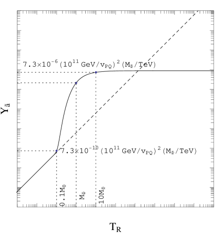
Figure 1: Relic axino number density over the entropy density vs the reheat temperature $T_{R}$ (solid line). The dashed line is the result one would get by using only the effective interaction (1).

Fig. 1 summarizes the results of our analysis. It shows $Y_{\tilde{a}}\propto T_{R}$ for $T_{R}\lesssim 0.1M_{\Phi}$, which is due to that axinos are produced mostly through the transition $g\rightarrow\tilde{g}+\tilde{a}$ or $\tilde{g}\rightarrow g+\tilde{a}$ when $T\lesssim 0.1M_{\Phi}$. If one uses only the effective interaction (1) to evaluate the axino production by $g\rightarrow\tilde{g}+\tilde{a}$ or $\tilde{g}\rightarrow g+\tilde{a}$, as one did in most of the previous analysis, one would get $Y_{\tilde{a}}\propto T_{R}$ even for $T_{R}\gtrsim 0.1M_{\Phi}$, as represented by the dashed line in Fig. 1. Taking it into account that the axino production at $T>M_{\Phi}$ is mostly due to the transition $\Phi\rightarrow\tilde{\Phi}+\tilde{a}$ or $\tilde{\Phi}\rightarrow\Phi+\tilde{a}$, one can easily understand the behavior of $Y_{\tilde{a}}$ for $T_{R}>10M_{\Phi}$, which is nearly independent of $T_{R}$. Note that the dashed line crosses the correct solid line at $T_{R}\sim 10^{3}M_{\Phi}$, implying that the previous analysis based on the effective interaction (1) alone gives rise to an overestimated axion relic density for the reheat temperature $T_{R}\gtrsim 10^{3}M_{\Phi}$, while it gives an underestimated $Y_{\tilde{a}}$ for $0.1M_{\Phi}\lesssim T_{R}\lesssim 10^{3}M_{\Phi}$.

4 Conclusion

For supersymmetric axion models which have a UV completion with linearly realized PQ symmetry at a fundamental scale $M_{*}\gg v_{PQ}$, the axion supermultiplet is decoupled from the gauge and matter supermultiplets in the limit $M_{\Phi}/v_{PQ}\rightarrow 0$ and $v_{PQ}/M_{*}\rightarrow 0$, where $M_{\Phi}$ is the mass of the heaviest PQ-charged and gauge-charged matter multiplet in the model. As a result, in models with small values of $M_{\Phi}/v_{PQ}$ and $v_{PQ}/M_{*}$, the axino production rate at temperature $T\gg M_{\Phi}$ is suppressed by the powers of small $M_{\Phi}/T$. This feature is particularly important for the cosmology of supersymmetric DFSZ axion model[5, 6] in which $M_{\Phi}$ corresponds to the MSSM Higgs $\mu$-parameter, so is far below $v_{PQ}$. Cosmology of KSVZ axion model can be significantly altered also, if the PQ-charged exotic quark has a mass well below $v_{PQ}$. One immediate consequence (see Fig. 1) is the relic axino density vs the reheat temperature for $0.1M_{\Phi}<T_{R}<v_{PQ}$, which is quite different from the previous result obtained using the effective interaction (1) alone.

References

• [1] For recent reviews, see L. Covi and J. E. Kim, New J. Phys.  11, 105003 (2009); F. D. Steffen, Eur. Phys. J.  C 59, 557 (2009).
• [2] See for instance K. Choi, E. J. Chun, J. E. Kim, Phys. Lett.  B403, 209 (1997); K. Choi, K. S. Jeong, W. -I. Park and C. S. Shin, JCAP 0911, 018 (2009); J. Fan, M. Reece and L. -T. Wang, JHEP 1109, 126 (2011).
• [3] E. J. Chun, H. B. Kim, J. E. Kim, Phys. Rev. Lett.  72, 1956 (1994); C. Cheung, G. Elor and L. J. Hall, Phys. Rev. D 85, 015008 (2012); A. Freitas, F. D. Steffen, N. Tajuddin and D. Wyler, JHEP 1106, 036 (2011).
• [4] L. Covi, H. B. Kim, J. E. Kim and L. Roszkowski, JHEP 0105, 033 (2001); L. Covi, L. Roszkowski and M. Small, JHEP 0207, 023 (2002); A. Brandenburg, F. D. Steffen, JCAP 0408, 008 (2004); A. Strumia, JHEP 1006, 036 (2010).
• [5] K. J. Bae, K. Choi and S. H. Im, JHEP 1108, 065 (2011).
• [6] K. J. Bae, E. J. Chun and S. H. Im, arXiv:1111.5962 [hep-ph].