Transport properties of a multichannel Kondo dot in a magnetic field

Abstract

We study the nonequilibrium transport through a multichannel Kondo quantum dot in the presence of a magnetic field. We use the exact solution of the two-loop renormalization group equation to derive analytical results for the $g$ factor, the spin relaxation rates, the magnetization, and the differential conductance. We show that the finite magnetization leads to a coupling between the conduction channels which manifests itself in additional features in the differential conductance.

Introduction.—The study of a localized spin coupled via an antiferromagnetic exchange interaction $J$ to $K$ independent electronic reservoirs has a long history in condensed matter physics.Hewson93 In the simplest case of $K=1$ the electron spins completely screen the local spin at low energies and thus lead to a Fermi liquid. In a renormalization group (RG) analysis this situation is characterized by the divergence of the renormalized exchange coupling $J(\Lambda)$ at the Kondo scale $\Lambda=T_{\text{K}}$. The situation is completely changedNozieresBlandin80 if the spin is coupled to more than one screening channel ($K>1$). Then the renormalized exchange coupling stays finite and flows to a non-trivial fixed pointNozieresBlandin80 ; Gan94 $J^{*}\sim 1/K$ at low energies, which manifests itself in unusual non-Fermi liquid behavior like a non-integer “ground-state degeneracy” or characteristic power laws in various observables.AndreiDestri84prl ; AffleckLudwig93

The recent developments in the ability to engineer devices on the nanoscale lead to the experimental realizationPotok-07 of two-channel Kondo physics in a quantum dot set-up.OregGoldhaber-Gordon03 In this set-up it was possible to measure the differential conductance and observe universal scaling and square-root behavior which are characteristic for the two-channel Kondo effect. This triggered theoretical studies2CK ; MitraRosch11 ; Eflow of the transport properties of multichannel systems using conformal field theory as well as numerical and perturbative RG methods. The latter uses a perturbative expansion in the renormalized exchange coupling which is well-controlled provided $K\gg 1$. Specifically, Mitra and RoschMitraRosch11 calculated the differential conductance, the splitting of the Kondo resonance in the $T$ matrix, and the current-induced decoherence in the absence of a magnetic field. Recently the spin dynamics was studiedEflow in the absence of a bias voltage and shown to possess pure power-law decay with an exponent $g=4/K$.

In this Brief Report we extend the analysis of Mitra and RoschMitraRosch11 to include an external magnetic field. We perform a real-time RG (RTRG) analysisSchoeller09 to derive the renormalized magnetic field, the spin relaxation rates, the magnetization of the quantum dot, and the current. In particular, we focus on inelastic cotunneling processes which lead to characteristic features in the differential conductance whenever one of the applied bias voltages $V_{i}$’s equals the value of the renormalized magnetic field. We further show that the finite magnetization on the dot leads to a coupling of the conduction channels which results in additional features in the differential conductance.

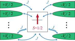
Figure 1: (Color online) Sketch of the $K$-channel Kondo model (1). The channels are labeled by $i=1,\ldots,K$, each channel is decomposed into two leads $\alpha=L,R$ held at chemical potentials $\mu_{L/R}^{i}=\pm V_{i}/2$. The spin-1/2 on the dot is subject to a magnetic field $h_{0}$. The exchange interaction $J$ between dot and leads present in all channels is depicted for the $K$th channel explicitly.

Model.—We consider a quantum dot possessing a spin-1/2 degree of freedom, which is coupled via an exchange interaction $J$ to $K$ independent electronic reservoirs. At low energies each reservoir constitutes one screening channel for the local spin thus leading to an over-screened situation for $K>1$. We will thus use the terms reservoir and channel interchangeably. Furthermore, the spin-1/2 is subject to an external magnetic field $h_{0}$. Each reservoir consists of a left ($L$) and right ($R$) lead which are held at chemical potentials $\mu_{\alpha}^{i}$, $\alpha=L,R$, $i=1,\ldots,K$ (see Fig. 1). Specifically we consider the system

$$\begin{split}H=&\sum_{i\alpha k\sigma}\epsilon_{k}\,c_{i\alpha k\sigma}^{\dagger}c_{i\alpha k\sigma}+h_{0}\,S^{z}\\ &+\frac{J_{0}}{2\nu_{0}}\sum_{i\alpha\alpha^{\prime}kk^{\prime}\sigma\sigma^{\prime}}\vec{S}\cdot\vec{\sigma}_{\sigma\sigma^{\prime}}c_{i\alpha k\sigma}^{\dagger}c_{i\alpha^{\prime}k^{\prime}\sigma^{\prime}}.\end{split}$$ (1)

Here $c_{i\alpha k\sigma}^{\dagger}$ and $c_{i\alpha k\sigma}$ create and annihilate electrons with momentum $k$ and spin $\sigma=\uparrow,\downarrow$ in lead $\alpha$ of the reservoir $i$, $\vec{\sigma}$ denotes the Pauli matrices, and $\vec{S}$ is the spin-1/2 operator on the dot. The antiferromagnetic exchange coupling $J_{0}>0$ is dimensionless in our convention. We stress that the exchange term does not couple different reservoirs. The chemical potentials in the leads are parametrized by $\mu_{L/R}^{i}=\pm V_{i}/2$ thus applying a bias voltage $V_{i}$ to each reservoir. Furthermore we introduce an ultra-violet cutoff $D$ in each reservoir via the density of states $N(\omega)=\nu_{0}D^{2}/(D^{2}+\omega^{2})$. In the absence of a magnetic field the transport properties of the model (1) have been previously studied in Ref. MitraRosch11, .

RG analysis.—Following Ref. Schoeller09, we have performed a two-loop RTRG analysis including a consistent derivation of the relevant relaxation rates. This method has been successfully applied to study transport properties of other Kondo-type quantum dots in the past.Schoeller09 ; PS11 The starting point is an RG equation for the renormalized exchange coupling $J(\Lambda)$ obtained by integrating out the high-energy degrees of freedom in the reservoirs. To accomplish this the one introduces a cutoff $\Lambda$ into the Fermi function and integrates out the Matsubara poles on the imaginary axis by decreasing the cutoff from its initial value $\Lambda_{0}\sim D$ down to some physical energy scale. The RG equation for the $K$-channel model (1) reads up to two loop

$$\Lambda\frac{d}{d\Lambda}J=\beta(J)=-2J^{2}(1-KJ),$$ (2)

which defines the reference solution $J(\Lambda)$ for our analysis. The RG flow has the well-knownNozieresBlandin80 non-trivial fixed point $J^{*}=1/K$. The scaling dimension of the leading irrelevant operator is $\Delta=\beta^{\prime}(J^{*})=2/K$, which is valid for $K\gg 1$ while the exact result is given byAffleckLudwig93 $\Delta=2/(K+2)$. The RG equation possesses the invariant

$$T_{\text{K}}=\Lambda_{0}\left(\frac{eJ_{0}}{J^{*}-J_{0}}\right)^{K/2}e^{-1/2J_{0}},$$ (3)

which defines the Kondo temperature. With the initial condition $J_{0}=J(\Lambda_{0})$ the solution of the RG equation can be explicitly written as

$$J(\Lambda)=\frac{J^{*}}{1+W(z)},\quad z=\left(\frac{\Lambda}{T_{\text{K}}}\right)^{\Delta}.$$ (4)

Here $W(z)$ denotes the Lambert W functionCorless96 defined by $z=W(z)e^{W(z)}$, which satisfies $W^{\prime}(z)={W(z)/z/(1+W(z))}$ for $z\neq 0$. The fixed point $J^{*}$ is reached for $\Lambda\to 0$ as $W(0)=0$. We note that the solution (4) is valid for all $J_{0}$ but, of course, the derivation of (2) requires $J_{0}\ll 1$. If $J_{0}<J^{*}$ we can perform the scaling limit $\Lambda_{0}\to\infty$ and $J_{0}\to 0$ while keeping the Kondo temperature constant. In this limit the solution for $\Lambda\ll T_{\text{K}}$ simplifies to

$$J(\Lambda)=J^{*}\left[1-\left(\frac{\Lambda}{T_{\text{K}}}\right)^{\Delta}\right],$$ (5)

i.e. there is a characteristic power-law behavior. Observables are calculated in a systematic expansion around the reference solution and can be expressed in terms of the renormalized exchange coupling $J_{c}\equiv J(\Lambda_{c})$ at the physical energy scalescale (we consider $T=0$)

$$\Lambda_{c}=\max\{V,h_{0}\}.$$ (6)

In contrast to the one-channel Kondo model the existence of the attractive fixed point $J^{*}=1/K$ implies that this expansion is well-defined for all $\Lambda_{c}$ provided $K\gg 1$. We have calculated the effective dot Liouvillian and the current kernel yielding the renormalized magnetic field, the spin relaxation rates, the dot magnetization, and the current including the leading logarithmic corrections. All calculations follow Ref. Schoeller09, , we present here only the results and discuss their properties.

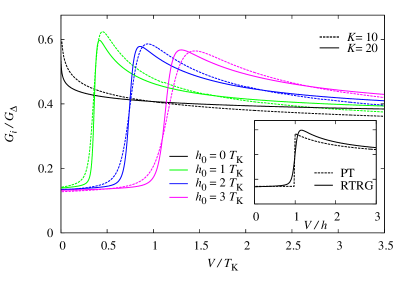
Figure 2: (Color online) Differential conductance of an individual channel for identical bias voltages $V_{i}=V$ and $K=10$ (dashed lines) or ${K=20}$ (solid lines) channels. We use the normalization $G_{\Delta}=(\frac{2e^{2}}{h})\frac{3\pi^{2}}{16}\Delta^{2}$. For zero field one findsMitraRosch11 $G/G_{\Delta}=1-2(V/T_{\text{K}})^{\Delta}$, i.e. $G/G_{\Delta}\to 1$ for $V\to 0$. Inset: Comparison of RTRG (solid line) and renormalized perturbation theory (PT) up to $\mathcal{O}(J_{c}^{2})$ (dashed line) for $h_{0}=T_{\text{K}}$ and $K=20$. We note that the broadening of the feature at $V=h$ is not captured in PT.

Identical bias voltages.—First let us assume that all bias voltages are identical, i.e. $V_{i}=V$. Straightforward calculation yields the renormalized magnetic field

$$h=\bigl{[}1-K(J_{c}-J_{0})\bigr{]}h_{0},$$ (7)

which gives for the $g$ factor in leading order (we consider the scaling limit $J_{0}\to 0$ from now)

$$g=2\frac{\partial h}{\partial h_{0}}=2(1-KJ_{c})\stackrel{{\scriptstyle\Lambda_{c}\ll T_{\text{K}}}}{{=}}2\left(\frac{\Lambda_{c}}{T_{\text{K}}}\right)^{\Delta}.$$ (8)

The longitudinal and transverse spin relaxation rates

$$\Gamma_{1} = \pi\left[h+\frac{1}{2}\big{(}\left|V-h\right|_{2}+V+h\big{)}\right]KJ_{c}^{2},$$ (9)

$$\Gamma_{2} = \frac{\pi}{2}\left[V+h+\frac{1}{2}\big{(}\left|V-h\right|_{1}+V+h\big{)}\right]KJ_{c}^{2},$$ (10)

with

$$\left|x\right|_{l}=\frac{2}{\pi}x\arctan\frac{x}{\Gamma_{l}},\quad l=1,2.$$ (11)

We note that for $\Lambda_{c}\gg T_{\text{K}}$ the renormalization of the magnetic field (7) is much stronger than in the one-channel Kondo model, as the spin on the dot is coupled to more screening channels.

Explicit formulas for the dot magnetization and the current are given in Eq. (14) below for the case of different bias voltages. Simplifying to $V_{i}=V$ we obtain the differential conductance $G_{i}=dI_{i}/dV_{i}$ per channel, which is plotted in Fig. 2. The conductance sharply increases around $V=h$ where inelastic cotunneling processes start to contribute. Due to the strong renormalization of the magnetic field the increase occurs at voltages much smaller than the applied magnetic field $h_{0}$. Close to the resonance we find

$$G_{i}=\begin{cases}\frac{\pi}{4}J_{c}^{2}\bigl{[}1+2J_{c}\mathcal{L}_{2}\big{(}V-h\big{)}\bigr{]}&\text{for }V<h,\\[5.69054pt] \pi J_{c}^{2}\bigl{[}1+2\pi J_{c}\mathcal{L}_{2}\big{(}V-h\big{)}\bigr{]}&\text{for }V>h,\end{cases}$$ (12)

where we assumed $|V-h|\ll h$ and defined

$$\mathcal{L}_{l}\big{(}x\big{)}=\ln\frac{\Lambda_{c}}{\sqrt{x^{2}+\Gamma_{l}^{2}}},\quad l=1,2.$$ (13)

We note that (12) is formally identical to the differential conductance in the one-channel Kondo modelSchoeller09 except for the functional form of the renormalized coupling (5). In particular, there is no explicit dependence on the number of channels. We further note that close to the fixed point the conductance (12) is a quantity of order $1/K^{2}$. The logarithmic divergencies at $V=h$ are cut off by the transverse spin relaxation rate $\Gamma_{2}$. Thus, as $\Gamma_{2}\sim 1/K$, this feature becomes sharper with increasing $K$. At small voltages $V<h$ the conductance is independently of the bias voltage given by $G_{i}=\pi J_{c}^{2}/4$. In particular, a power-law behavior in the voltage is only found for vanishing magnetic fieldMitraRosch11 while (5) yields a power-law dependence on the magnetic field. In the limit of a large field $h\gg T_{\text{K}}$ the linear conductance can be derived usingCorless96 $W(z)\sim\ln z$ for $z\to\infty$ to be $G_{i}(V=0,h)=\pi/16/\ln^{2}(h/T_{\text{K}})$, which is identical to the result in the one-channel model.

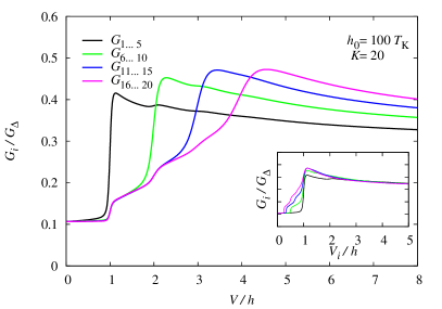
Figure 3: (Color online) Differential conductance $G_{i}$ through channel $i$ for $h_{0}=100\,T_{K}$ and $K=20$. The bias voltages are applied such that series of five channels have identical voltages, i.e. $V_{i}=a_{i}V$ with $a_{1,\ldots,5}=1$, $a_{6,\ldots,10}=1/2$, $a_{11,\ldots,15}=1/3$, and $a_{16,\ldots,20}=1/4$. For $h_{0}=0$ the conductance is similar to the black curve in Fig. 2, i.e. there are no features. Inset: Same situation as in the main panel, but plotted with respect to the respective bias voltage $V_{i}$.

Different bias voltages.—In the following we relax the condition $V_{i}=V$ and consider channel-dependent bias voltages $V_{i}$. This introduces further energy scales which will give rise to additional features in the dot magnetization and thus the differential conductance. In this general set-up the magnetization and current through the $i$th channel are given by

$$M=-\frac{f_{1}}{2f_{2}},\quad I_{i}=f_{I}^{i}+2Mf_{M}^{i}$$ (14)

where $f_{1,2}$ denote rates appearing in the Liouvillian and $f^{i}_{I,M}$ are similar terms in the current kernel. Explicitly these rates read

$$f_{1} = 2\pi KJ_{c}^{2}h+4\pi KJ_{c}^{3}h\mathcal{L}_{2}\big{(}h\big{)}$$ (15)

$$-2\pi J_{c}^{3}\sum\nolimits_{j=1\ldots K}(V_{j}-h)\mathcal{L}_{2}\big{(}V_{j}-h\big{)},$$

$$f_{2} = \pi KJ_{c}^{2}h+2\pi KJ_{c}^{3}h\mathcal{L}_{2}\big{(}h\big{)}$$

$$\* +\frac{\pi}{2}J_{c}^{2}\sum\nolimits_{j=1\ldots K}\big{(}\left|V_{j}-h\right|_{2}+V_{j}+h\big{)}$$

$$+\pi J_{c}^{3}\sum\nolimits_{j=1\ldots K}\big{(}\left|V_{j}-h\right|_{2}-V_{j}+h\big{)}\mathcal{L}_{2}\big{(}V_{j}-h\big{)},$$

$$f_{I}^{i} = \frac{3}{4}\pi J_{c}^{2}V_{i}+\pi J_{c}^{3}V_{i}\mathcal{L}_{1}\big{(}V_{i}\big{)}$$ (17)

$$+\pi J_{c}^{3}(V_{i}-h)\mathcal{L}_{2}\big{(}V_{i}-h\big{)},$$

$$f_{M}^{i} = -\frac{\pi}{4}J_{c}^{2}\big{(}\left|V_{i}-h\right|_{2}-V_{i}-h\big{)}+\pi J_{c}^{3}V_{i}\mathcal{L}_{1}\big{(}V_{i}\big{)}$$ (18)

$$+\pi J_{c}^{3}h\mathcal{L}_{2}\big{(}h\big{)}-\frac{\pi}{2}J_{c}^{3}\left|V_{i}-h\right|_{2}\mathcal{L}_{2}\big{(}V_{i}-h\big{)}.$$

The relaxation rates for the case of different bias voltages are obtained by straightforward generalization of Eqs. (9) and (10). In the derivation of Eqs. (15)–(18) we have neglected all terms in order $J_{c}^{3}$ that do not contain logarithms at either $h=0$, $V=0$, or $V=h$. Thus when calculating the magnetization one has to expand consistently up to this order.

Figure 4: Derivative of the magnetization with respect to the voltage, i.e. $\partial M/\partial V$. All parameters are as in Fig. 3. We observe pronounced features at $V=h$ and $V=2h$. Inset: Magnetization as a function of the bias voltage.

We stress that although the different channels are not directly coupled via exchange interactions, the finite magnetization $M$ mediates a feedback between them. Consider for example the differential conductance of channel 1, i.e. the black curve in Fig. 3. The sharp increase at $V=V_{1}=h$ is again due to the onset of inelastic cotunneling processes. However, there is a second feature at $V\approx 2h$ which is caused by the non-trivial voltage dependence of the dot magnetization. This can be seen in the derivative $\partial M/\partial V$ shown in Fig. 4, which directly enters the differential conductance [see (14)]. Similarly, the conductance in channel 6 (green curve in Fig. 3) possesses a feature at $V=2V_{6}=h$ which is caused by the effect of the applied voltage in channels 1 to 5 onto $M$, while the increase at $V_{6}=h$ (i.e. $V=2h$) is due to the onset of inelastic cotunneling in channel 6. In this way the nonequilibrium magnetization introduces additional features into the individual conductances. We stress that such coupling effects between the channels are absent for vanishing magnetic fieldMitraRosch11 or if all applied bias voltages are identical (see Fig. 2).

As a special case of the general set-up with channel-dependent bias voltages we can recover the experimental situation realizedPotok-07 by Potok et al. in a semiconductor quantum dot. This is achieved by setting the chemical potentials to $\mu_{L/R}^{1}=\pm V/2$ and $\mu_{L/R}^{i}=0$ for $i=2,\ldots,K$. In each of the channels $2,\ldots,K$ we introduce even and odd combinations of the electron operators, $(c_{iLk\sigma}\pm c_{iRk\sigma})/\sqrt{2}$, such that the even combinations couple to the spin on the dot with exchange interaction $2J$ while the odd ones decouple completely. The resulting RG equation for $J$ is given by (2) and thus possesses the fixed point $J^{*}$. The experimental set-up Potok-07 is now obtained by specializing to $K=2$. In the presence of a magnetic field the resulting differential conductance is very similar to the case of identical bias voltages shown in Fig. 2. In particular, since the second channel does not provide an additional energy scale there appear no features in the differential conductance beside the cotunneling peak at $V=h$. A possible experimental set-up to observe the additional features shown in Fig. 3 thus requires at least two channels with non-zero and different bias voltages.

Conclusions.—To sum up, we have studied the nonequilibrium transport properties of a multichannel Kondo quantum dot in the presence of a magnetic field. We used the solution of the two-loop RG equation to derive analytical results for the $g$ factor, the spin relaxation rates, the dot magnetization, and the differential conductance. The latter shows typical features of inelastic cotunneling. We showed that the main difference to the previously studiedMitraRosch11 situation without magnetic field is the appearance of additional features in the differential conductance, which originate in the feedback between the channels mediated by the finite dot magnetization.

We thank S. Andergassen, A. Rosch, and H. Schoeller for useful discussions. This work was supported by the German Research Foundation (DFG) through the Emmy-Noether Program.

References

- (1) A. C. Hewson, The Kondo Problem to Heavy Fermions (Cambridge University Press, Cambridge, 1993).
- (2) P. Nozières and A. Blandin, J. Phys. France 41, 193 (1980).
- (3) J. Gan, N. Andrei, and P. Coleman, Phys. Rev. Lett. 70, 686 (1993); J. Gan, J. Phys.: Condens. Matter 6, 4547 (1994).
- (4) N. Andrei and C. Destri, Phys. Rev. Lett. 52, 364 (1984); A. M. Tsvelick and P. B. Wiegmann, Z. Phys. B 54, 201 (1984); I. Affleck and A. W. W. Ludwig, Phys. Rev. Lett. 67, 161 (1991).
- (5) A. W. W. Ludwig and I. Affleck, Phys. Rev. Lett. 67, 3160 (1991); I. Affleck and A. W. W. Ludwig, Phys Rev. B 48, 7297 (1993).
- (6) R. M. Potok, I. G. Rau, H. Shtrikman, Y. Oreg, and D. Goldhaber-Gordon, Nature (London) 446, 167 (2007).
- (7) Y. Oreg and D. Goldhaber-Gordon, Phys. Rev. Lett. 90, 136602 (2003).
- (8) A. I. Tóth, L. Borda, J. von Delft, and G. Zaránd, Phys. Rev. B 76, 155318 (2007); R. Žitko and J. Bonča, ibid. 77, 245112 (2008); E. Sela and I. Affleck, Phys. Rev. Lett. 102, 047201 (2009); E. Vernek, C. A. Büsser, G. B. Martins, E. V. Anda, N. Sandler, and S. E. Ulloa, Phys. Rev. B 80, 035119 (2009); A. K. Mitchell and D. E. Logan, ibid. 81, 075126 (2010); E. Sela, A. K. Mitchell, and L. Fritz, Phys. Rev. Lett. 106, 147202 (2011); A. K. Mitchell, D. E. Logan, and H. R. Krishnamurthy, Phys. Rev. B 84, 035119 (2011); A. K. Mitchell, E. Sela, and D. E. Logan, Phys. Rev. Lett. 108, 086405 (2012); A. K. Mitchell and E. Sela, e-print arXiv:1203.4456.
- (9) A. Mitra and A. Rosch, Phys. Rev. Lett. 106, 106402 (2011).
- (10) M. Pletyukhov and H. Schoeller, e-print arXiv:1201.6295.
- (11) H. Schoeller, Eur. Phys. J. Special Topics 168, 179 (2009); H. Schoeller and F. Reininghaus, Phys. Rev. B 80, 045117 (2009); ibid. 80, 209901(E) (2009).
- (12) D. Schuricht and H. Schoeller, Phys. Rev. B 80, 075120 (2009); M. Pletyukhov, D. Schuricht, and H. Schoeller, Phys. Rev. Lett 104, 106801 (2010); M. Pletyukhov and D. Schuricht, Phys. Rev. B 84, 041309(R) (2011); C. B. M. Hörig, D. Schuricht, and S. Andergassen, ibid. 85, 054418 (2012).
- (13) R. M. Corless, G. H. Gonnet, D. E. G. Hare, D. J. Jeffrey, and D. E. Knuth, Adv. Comput. Math. 5, 329 (1996).
- (14) For the numerical evaluation we use .