Mesoscopic Biochemical Basis of Isogenetic Inheritance and Canalization: Stochasticity, Nonlinearity, and Emergent Landscape

Abstract

Biochemical reaction systems in mesoscopic volume, under sustained environmental chemical gradient(s), can have multiple stochastic attractors. Two distinct mechanisms are known for their origins: ($a$) Stochastic single-molecule events, such as gene expression, with slow gene on-off dynamics; and ($b$) nonlinear networks with feedbacks. These two mechanisms yield different volume dependence for the sojourn time of an attractor. As in the classic Arrhenius theory for temperature dependent transition rates, a landscape perspective provides a natural framework for the system’s behavior. However, due to the nonequilibrium nature of the open chemical systems, the landscape, and the attractors it represents, are all themselves emergent properties of complex, mesoscopic dynamics. In terms of the landscape, we show a generalization of Kramers’ approach is possible to provide a rate theory. The emergence of attractors is a form of self-organization in the mesoscopic system; stochastic attractors in biochemical systems such as gene regulation and cellular signaling are naturally inheritable via cell division. Delbrück-Gillespie’s mesoscopic reaction system theory, therefore, provides a biochemical basis for spontaneous isogenetic switching and canalization.

1 Introduction

Epigenetic inheritance at the cellular level preserves certain phenotypes through cell divisions [[31]]. Since the definition of “epigenetic” means the inheritability is not due to genes, i.e., DNA sequences, the epigenetic phenomenon must be a biochemical process [[39, 53]]. DNA and histone modifications, gene regulations by transcriptional factors, signaling networks, and metabolic pathways are all parts of cellular biochemistry. Current research chiefly focuses on the “code” of epigenetic inheritance in terms of DNA methylation and/or histone acetylation [[56, 29, 36]].

While the gene expressions and their regulations are a central component of epigenetic processes, it is less certain what the roles of cellular signaling networks, or metabolic networks, are. Even more importantly, are different gene expressions the cause of the epigenetic phenomenon, or consequences of the dynamics of a larger intracellular biochemical network as a whole? In the present paper, we advance a theory for biochemical reaction systems in a mesoscopic volume [[42]]. Taking a broader perspective that is rooted in stochastic, nonlinear dynamical systems [[43]], we illustrate that it is likely that the code for epigenetic inheritance is distributive [[26]]. Using two classes of biochemical networks (see Fig. 1) as illustrations, we investigate mesoscopic, nonlinear biochemical reaction networks with multiple stochastic attractors [[60]]. More importantly, we shall show that two very different types of mesoscopic bistabilities exist: the stochastic bistability which has no macroscopic counterpart [[30, 50, 27, 49, 63, 6]], and the nonlinear bistability which exhibits deterministic bistability when the system’s volume tends to macroscopic scale [[58, 19, 35, 51]].

There is a growing awareness of mesoscopic biochemical bistability [[37, 14, 55, 12, 9]]. Multistability in a mesoscopic chemical reaction system can be mathematically represented by the Delbrück-Gillespie processes (DGP) whose probability distribution function follows chemical master equation [[13]] and whose exact stochastic trajectories can be obtained by the widely known Gillespie algorithm [[3, 25]]. This approach has found numerous applications in recent studies. For an introduction to this chemical reaction system theory, see [[43, 42, 35, 48, 62, 5]]. A review by [46] is particularly accessible.

In principle, a biochemical reaction system in a small volume of the size of a cell, on a very large time scale (years, hundreds years), will have a steady state probability distribution which reflects the continuous jumping among the multiple stochastic attractors: regions with high local probability [[20, 19, 66]]. In terms of this stationary distribution, the dynamics of a mesoscopic biochemical system can be cogently visualized and even quantified by a landscape representation [[18, 66, 61, 28, 21]].

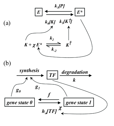
Figure 1: A biochemical signaling network of phosphorylation-dephosphorylation cycle (PdPC) and gene expression regulatory network for a self-regulating gene are essentially isomorphic. (a) An enzyme $E$ can be phosphorylated to become $E^{*}$, catalyzed by a kinase $K$. Dephosphorylation of $E^{*}$ is catalyzed by phosphatase $P$. The activity of $K$, however, is modified through binding $\chi$ copies of $E^{*}$: $K^{{\dagger}}$ denotes $K(E^{*})_{\chi}$ complex. (b) The expression of a transcription factor (TF) is regulated by the very TF, in monomer or dimer form ($\chi=1,2$). The TF is degradated with rate $k$. $g_{1}$ and $g_{0}$ are the respective biosynthesis rates when the TF is on and off the gene. If $g_{1}<g_{0}$, the TF is a repressor; and if $g_{1}>g_{0}$ the TF is an activator. [Redrawn based on Fig. 14 of [23].]

It will be illustrated in this paper that multistability is not only stable against noise, i.e., robust, but also could be readily inherited during the process of cell volume change and division. Within a cell cycle, it is not necessary to directly control the concentration of a biochemical species: As soon as cellular concentrations are deviated from their locally most stable values, the dynamics will cause them to spontaneously relax back as long as the deviations are within the limit of the basin of the attraction (stable state). Indeed, this restoring phenomenon should be regarded as a form of “self-organization”. Such state naturally has stability and robustness. On the larger landscape scale, the system is “digital”. This kind of “inheritable code” is not only distributive but also dynamic [[26]], in contrast to Watson-Crick basepairng.

Some mathematical analysis of the DGP is at the foundation of our current landscape theory [[42, 43]]. In Sec. 4 we offer some discussions. Intuitive and appealing as it is, the justification of using the stationary probability distribution as the landscape involves subtle mathematical ideas which deserves further investigations [[20, 21]].

2 Biosynthesis of Self-regulating Repressor with Slow On-and-off Gene Fluctuations

We first consider a simple model for the biosynthesis and degradation of a repressor with stochastic gene expression, which is regulated by the repressor. The canonical kinetic scheme for this model, neglecting the intermediate stage of mRNA, is in Fig. 1b. For simplicity, we assume that the repressor-gene binding rate $h(n)=h_{o}n$ which involves a monomer, and $g_{0}>g_{1}$. See [30], [50] [27], and [60] for extensive studies of this model, and related systems with self-activation dimer ($h(n)\propto n(n-1)$, $g_{1}>g_{0}$). We choose this model to demonstrate bistability due to slow, nonadiabatic fluctuations in the gene state. This is a stochastic effect due to single-molecule behavior [[4, 63]] which disappears in the macroscopic Law of Mass Action [[27, 47]] (see Methods).

2.1 Stochastic bimodality and bistability

It is generally accepted that, in biochemistry, noise-induced bistability means a small kinetic system has bimodal distribution while its macroscopic counterpart has only uni-stability [[27, 49, 6]]. Usually, the meaning of “macroscopic counterpart” is defined as the same chemical or biochemical reaction systems at same concentrations. For a large volume, the concentrations are deterministic variables; but in a mesoscopic volume, the copy numbers fluctuate. This “correspondence principle” is consistent with the experimental practices: In the past most biochemical experiments on gene expression were carried out with DNA measured in concentrations [[59]].

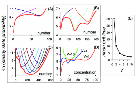
Figure 2: Steady state probability distributions for the repressor molecule numbers in mesoscopic systems with different volume $V$ but same DNA concentration $x_{t}=1$. (A) One gene with $V=1$. The red curve is the repressor distribution. The two thin curves are $p^{ss}(n|m)$ with $m=1,0$. Model parameters are taken from [27]. (B) Four genes with $V=4$. The thin curves are for $p^{ss}(n|m)$ with $m=4,3,2$. (C) Ten genes with $V=10$. (D) Distributions for the concentration of the repressor protein as functions of increasing $V$ approaching to the macroscopic prediction with steady state at $y^{*}=27.8$ (see Methods). (E) The mean exit time for the all-off, low-transcription state, defined when possible as the well at $n=Mg_{1}/k=(g_{1}x_{t}/k)V$, decreases with $V$.

With increasing volume of the a reaction system ($V$) and the copy numbers DNA ($M$), stability of one of the two states decreases while the other increases. For a sufficiently large $V$, the bistability disappears all together [[27, 47]]. We call such bistability stochastic bistability. Fig. 2 shows how the stationary probability distributions change with the increasing $V$ and DNA copy number $M$ while keeping its concentration $x_{t}=M/V=1$.

In agreement with the visual landscapes in Figs. 2A-D, 2E also shows how the mean sojourn time for the all-off, low transcription state ($m=0,n\leq 80$ in Eq. 6.1) decreases as a function of $V$. This is in sharp contrast to the nonlinear bistability (Fig. 5) we shall discuss next.

3 Phosphorylation Dephosphorylation Cycle with Nonlinear Feedbacks

A gene regulatory network with dimeric activator also exhibits bistability [[30, 60, 51]], but by a different mechanism. To illustrate this, and also to broaden the scope of our discussions, we shall consider a cellular phosphorylation dephosphorylation cycle (PdPC) signaling network in Fig. 1a. In particular, we shall consider the case of positive feedback with a dimer ($\chi=2$). The same analysis can be applied to the gene expression system with $\chi=2$ and $g_{1}>g_{0}$ in Fig. 1b. It is easy to show that for $\chi=0,1$, the cellular signaling network in Fig. 1a, with slow fluctuating kinase activity, exhibits stochastic bistability [[6, 47]]. The theory we present here is general to both types of biochemical networks in terms of nonlinear chemical kinetics.

The class of networks in Fig. 1a has been widely implicated, such as in Src family kinase membrane signaling [[11]], Rab 5 GTPase in endocytic pathway [[65]], Xenopus oocytes regulation for cell fate [[15]], and long-term neural memory [[37, 9]]. The network has been studied in [16, 45, 19, 6]. The detailed kinetic scheme is given in Eq. 1 for which a DGP is uniquely specified (see Methods):

$$E+K^{{\dagger}}+ATP\overset{k_{1}}{\underset{k_{-1}}{\rightleftharpoons}}E^{*}+K^{{\dagger}}+ADP,$$ (1)

$$K+2E^{*}\overset{k_{2}}{\underset{k_{-2}}{\rightleftharpoons}}K^{{\dagger}},\ \ \ E^{*}+P\overset{k_{3}}{\underset{k_{-3}}{\rightleftharpoons}}E+P+Pi.$$

Note that the stochastic Delbrück-Gillespie approach is not an alternative to the traditional enzyme kinetic modeling (Eqs. 10, 11). When copy numbers in a chemical reaction system are large, a Delbrück-Gillespie process (DGP) automatically yields the deterministic dynamics predicted by the traditional Law of Mass Action [[5, 46]]. One of the most important predictions of the DGP theory is a dynamic landscape for the system, as shown in Fig. 3 as well as Figs. 2A-D. Such a landscacpe can only be rigorously defined in a stochastic model; it can be computed using a chemical master equation.

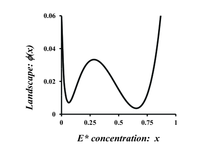
Figure 3: The landscape for the PdPC kinetic system in Eq. 1, $\phi(x)$, according to Eq. 16, using parameters $x_{t}=1$, $\alpha=43$, $\beta=10$, $\epsilon=0.01$ and $\delta=0.5$. From Eq. 11, the steady states are $x_{1}^{*}=0.05$ (stable), $x_{2}^{*}=0.632$ (stable), and $x_{3}^{*}=0.368$ (unstable).

4 Time Scales, Emergent Landscape and Implications to Epigenetics

4.1 Three time scales of cellular dynamics

Double-well landscapes shown in Figs. 2 and 3 suggest multiple time scales in the biochemical dynamics. In fact, there are three distinct time scales in such systems. Note that while fluctuations modify the “down-hill” deterministic kinetics, they lead to “up-hill” dynamics which is impossible in a macroscopic system. The time for “barrier crossing”, however, is extremely slow in comparison to the down-hill kinetics.

Therefore, the fast time scale in the system is the individual biomolecular reactions in Fig. 1. For the present work, they are given in terms of the rate parameters $k$’s in Fig. 1a and $f,g,h,k$ in Fig. 1b (or equivalently, the $\alpha,\beta,\epsilon,\delta$ in Eq. 9.) Millisecond are not unreasonable, even though individual biochemical reactions inside a cell could be much faster or slower.

The middle time scale is the relaxation kinetics of a network to its steady states, as illustrated in the Fig. 3 by the downhill dynamics. Note that the very existence of a steady state (an attractor), or steady states, is a consequence of “self-organization” of a complex reaction network.

The slow time scale is the transition rates between the two basins of attraction, or “wells”. Both the middle (deterministic) and slow (stochastic) time scales are emergent properties of the biochemical network. Following [23] we shall denote them molecular signaling time scale (MSts), biochemical network time scale (BNts), and cellular evolution time scale (CEts), respectively.

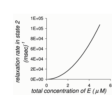
Figure 4: Relaxation kinetics in the state 2, the well on the right in Fig. 3 corresponding to state $x_{2}^{*}$, as a function of the total concentration of $E$, $x_{t}$, according to Eq. 12. The parameter used are $\alpha=4.3\mu sec^{-1}\mu M^{-2}$, $\beta=10msec^{-1}$, $\epsilon=1msec^{-1}\mu M^{-2}$ and $\delta=0.5msec^{-1}$.

Again taking the signaling system in Fig. 1a (also Eq. 1) as an example. For biochemically realistic situations, $\epsilon\ll\alpha$. We thus have the landscape given in Eq. 16 simplified into

$$\phi(x)=x_{t}\ln(x_{t}-x)-x\ln\left[\frac{(\alpha x^{2}+\delta)(x_{t}-x)}{\beta x}\right]$$

$$-2\sqrt{\frac{\delta}{\alpha}}\arctan\left(\sqrt{\frac{\alpha}{\delta}}x\right)+2x.$$ (2)

The parameters $\alpha,\beta,\delta$ in Eq. 2 define the MSts. We can now use the model to investigate the role of $\alpha,\beta$ and $\delta$ on the BNts and CEts. The BNts is given by the $r_{1}$ and $r_{2}$ in Eq. 12, and the CEts is given by the $T_{1\rightarrow 2}$ and $T_{2\rightarrow 1}$ in Eqs. 18-20.

The BNts changes with total concentrations of the regulators $E$ inside the system, as well as the concentrations of other factors. Fig. 4 shows how in the simple model the time-scale decrease, i.e., rate increases, with the total concentration of $E$, $x_{t}$. Within less than one order of magnitude change of $x_{t}$, from 1 to 6$\mu M$, the relaxation rate in the state 2, i.e., the well on the right in Fig. 3, increase by a factor of 100. Eq. 12 confirms that there is a square dependence of the relaxation rate to the concentration.

The CEts is extremely sensitive to the number of molecules in the biochemical system. Fig. 5 shows that with the MSts on the order of milli- and microsecond, and with concentration of $E$ on the order of micromolar , the transition times between the two states in Fig. 3 can be as long as thirty thousand years! Hence, the stability of the emergent attractors could be extremely robust against spontaneous concentration fluctuations (i.e., intrinsic noise) in the system. We also notice that both transition rates decrease with the $V$. This will be explained in Sec. 4.3 below.

More interesting biologically, we note that the range of 700-1000 copy number of $E$ corresponds to a time range of 10 hours to 30 years. In yeast, [24] have reported that the copy numbers for most of the transcription factors are centered arround $2^{10}=1024$ per cell.

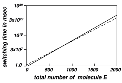
Figure 5: The switching times between two stable states, $T_{1\rightarrow 2}$ (dashed line) and $T_{2\rightarrow 1}$ (solid line) increase with the volume $V$ in nonlinear bistability (according to Eqs. 18). $x_{t}=0.1\mu M$, $\alpha=4.3\mu sec^{-1}$, $\beta=10msec^{-1}$, $\epsilon=1msec^{-1}$ and $\delta=0.5msec^{-1}$. A cell has a volume at about 10-20 femtoliter. With concentration $x_{t}=0.1\mu M$, there are 600-1200 number of total molecules. This gives the switching time around $3\times 10^{4}$ to $10^{12}$ sec. That is 10 hours to thirty thousand years! Therefore, with rather rapid individual biochemical reaction rates $\alpha$, $\beta$, $\epsilon$ and $\delta$, the emergent epigenetic states can be extremely stable.

4.2 Epigenetic inheritance and canalization on the CEts

Let us consider two replica of a mesoscopic biochemical reaction system in a laboratory, for example one of those in Fig. 1a which do not involve gene expression. If the two systems have same total $E$ but different initial values for $E^{*}$, one near zero and one near the total $E$, then these two systems settle to the two different attractors. In the time scale much shorter than the evolutionary transitions, the numbers of $E^{*}$ fluctuate around the $n_{1}^{*}$ and $n_{2}^{*}$, respectively, or equivalently around the $c_{1}^{*}$ and $c_{2}^{*}$ if the volume of systems do not change. (If the volumes are changing, then the fluctuations are around the $c_{1}^{*}$ and $c_{2}^{*}$, but not $n_{1}^{*}$ and $n_{2}^{*}$!) However, at the time scale greater than the cellular evolution, there will be transitions between the two attractors. This is shown in Fig. 6A. The probability distribution for the concentration of $E^{*}$ is shown in Fig. 6C.

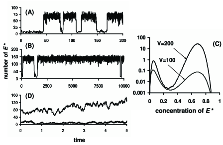
Figure 6: Nonequilibrium steady state fluctuation of the number of phosphorylated $E^{*}$ as functions of time, with $V=100$ in (A) and $V=200$ in (B). The steady state distributions of the number of $E^{*}$ for the $V=100,n_{t}=100$ and $V=200,n_{t}=200$ are shown in (C). The parameters used are $\alpha=43,\beta=10,\epsilon=0.01$ and $\delta=0.5$. (D) The volume $V$ and $n_{t}$ are increased by a factor of 2 from $V=100,n_{t}=100$ to $V=200,n_{t}=200$ within the time 0 to 5. One sees that the two attractors are well separated in the volume doubling process.

Fig. 6B shows the identical reaction system, except its volume and total $E$ are twice as large (keeping the concentration invariant). What we observe from the Fig. 6C is that the “concentration” distribution for $E^{*}$ in the two cases have essentially the same locations for the peaks and trough. This implies that if the size of the biochemical reaction system increases in the time scale sufficiently short, then the identities of the attractors can be preserved.

The stable state of the system is not only stable against intrinsic noise, but also could be readily transferred to the two daughter cells. During the cell cycle, the concentrations of biochemical substances might become approximately one half of the original value, in the extreme cases due to cell volume increase, and the system deviates from its corresponding stable state. The kinetic law of these two daughter systems is just the same as their mother cell except they have not relaxed to any of the stable states. As we have shown previously that the relaxation scale is not very large, so they will spontaneously relax back to the same corresponding stable state as long as not leaving an basin. Many previous work of epigenetics always searched for a stable chemical substance like DNA, which could be self-propagated and inherited to the daughter cells, while here we give another alternative possibility that the code of epigenetic is at the dynamic level of the whole biochemical network.

Further, there are clear upper and lower bounds for the rate of volume increase: it can not be too large such that the instantaneous changing concentration is outside the basin of an attractor; it can not be too slow such that it is on the cellular evolution time scale. Surely, the stability of epigenetic code is weaker than that for a stable chemical substance and it is more flexible facing the influence of the fluctuating environment, but it is suffient for a normal cell, a chemical system, to survive and inherit even in a fluctuating environment.

Fig. 6D shows precisely two of such simulations. Consider the volume, and the total $E$, double within the time of 5 units. This is a duration much shorter than the cellular evolution time. The top and bottom traces are the number of $E^{*}$ from two simulations. At the end of the doubling, if each system is divided into two, both “daughter systems” will also inherit the biochemical state of the “mother system”. The biochemistry of a mesoscopic reaction system is inheritable! The epigenetic stability, i.e., canalization [[36]] could be directly related to the CEts.

4.3 Mesoscopic stochastic dynamics on a landscape

The foregoing discussion clearly illustrates the power of the “landscape” perspective in visualizing and representing the global dynamics in bistable systems. We see that for stochastic bistability, at least one of the “barrier heights” decrease with volume $V$ (Fig. 2), while for nonlinear bistability, the both barrier heights increase with the volume (Figs. 5 and 6).

What determines the entire landscape? Since it is defined on the space for all possible concentrations and/or copy numbers of all the molecular species in the reaction system, itself can not be determined by the concentrations and copy numbers. Rather, it is determined by the all possible molecules involved and their interaction/reaction rate constants. In other words, biochemical reaction networks. Since the molecular interaction/reaction rate constants are properties of molecular structures, which in turn is determined by the primary sequences in the case of proteins, we conclude that the landscape, conceptually, is encoded in the DNA sequence, together with the extracellular environment including the volume $V$, but is independent of the expression patterns of transcription factors. They are the consequences of a biochemical reaction system’s dynamics [[50]].

There are many similarities between the energy landscape for a protein in equilibrium [[18]] and the landscape for an open mesoscopic chemical system in a nonequilibrium steady state [[66, 41, 23]]. We, however, want to emphasize a key difference: Recall that an energy landscape exists a priori for a dynamical protein [18]. The open-chemical systems are fundamentally different in this respect [[40, 41, 23]]. Specifically, for any finite volume $V$, a mesoscopic reaction system has a stationary probability distribution for the number of copies of all its biochemical species, $p_{V}({\bf n})$, where ${\bf n}=(n_{X},n_{Y},n_{Z},\cdots)$ are the copy numbers of the molecules $X,Y,Z$ etc. It can be shown that such a distribution can be expressed as

$$p_{V}({\bf n})=\exp\left[-V\phi({\bf x})+\phi_{1}({\bf x})+\frac{\phi_{2}({\bf x})}{V}+\cdots\right],$$ (3)

where ${\bf x}={\bf n}/V$. Furthermore, it can be shown that the function $\phi({\bf x})$ is a meaningful landscape for the complex dynamics of the nonlinear biochemical system. That is, the dynamics always goes “down the hill” of $\phi({\bf x})$ [[28, 21]], though usually not by the steepest descent path. As we have seen, the landscape provides an very useful organizational device for thinking about cellular biochemical dynamics at widely different time scales, ranging from individual signaling reactions to cellular phenotype switching.

Eq. 3 shows that the stationary distribution $p_{V}({\bf x})$ changes with $V$. When the $V$ becomes macroscopic volume, the probabilities are concentrated only at the global minima of the function $\phi({\bf x})$. However, with increasing $V$, $-(1/V)\ln p_{V}({\bf n})$ approach to the function $\phi({\bf x})$ which is defined on the entire space of ${\bf x}$. It is an important insight that such a landscape exist and it is independent of the system’s volume, as long as the volume is reasonably large [[28, 21]].

The nonlinear bistability, therefore, is the mesoscopic manifestation of a double well in the $\phi({\bf x})$. Its macroscopic counterpart has two stable steady states. However, stochastic bistability is something very different: The bimodal distribution only exists when the $V$ is sufficiently small; when $\phi_{1}$ and $\phi_{2}$ in Eq. 3 contribute to the $p_{V}({\bf n})$. $\phi({\bf x})$ has only a single well. With increasing volume: the barrier in the nonlinear bistability increases, while that of stochastic bistability decreases.

The emergent landscape of cellular interaction network dynamics and the landscape for protein dynamics are fundamentally different. The lack of detailed balance due to the open chemical nature of the former gives rise to the cycle flux underneath the landscape [[61, 23]]. The cycle flux makes the landscape non-local. When such a flux is sufficiently strong (i.e., mathematically characterized by the emerging of complex eigenvalue and eigenvectors), a synchronized dynamics arises [[44, 22]]. The emergence of synchronized dynamics requires an entirely new kind of phenomenology. In the macroscopic classical world, this is the birth of oscillatory behavior and wave phenomena that have ruled classical engineering for a century.

5 Discussion

5.1 Adaptive landscape

While the concept of energy landscape becoming a very useful term in protein dynamics, the concept of adaptive landscape in evolutionary dynamics is still highly controversial [[8]]. We believe one of the main reasons for this situation is that the landscape in the latter, as the landscape in the present work, is an emergent entity, which is not given a priori. There are two issues related to this important distinction: (1) The mathematical existence of such a landscape in a general, nonlinear stochastic dynamics which does not have detailed balance; and (2) How is such a landscape, even exists, related to the dynamics, both deterministic and stochastic. The most nontrivial issue here is the logical relationship between the landscape and the dynamics: It is rather clear that in systems with detailed balance, the landscape exists a priori and the dynamics is a consequence of the landscape. However, for system without detailed balance, the dynamics, as defined by the reaction networks and all the individual rate constants, define the overall dynamics as well as define the landscape. Dynamics and the landscape have correlations but no causality. Hence, logically, it is not correct to view the dynamics as a consequence of the landscape. Nevertheless, the landscape is still a very useful device to understand and characterize the overall dynamics. The concept of emergent landscape, thus, should only be understood in this “historically retrospective” sense.

5.2 Genocentric epigenetic inheritable memory and a possible alternative

Currently, methylation of DNA is considered to be the leading candidate for epigenetic inheritance. Even though this mechanism is not based on Watson-Crick basepairing, its function is still intimately dependent on the discovery of 1950s. Namely, the “code” is still a part of an extended, modified DNA structure. While certainly methylation is a part of the “whole picture” of epigenetic regulation, such a view might be too genocentric and too limited. It is not unlikely that the code of epigenetic inheritance is dynamics rather than static, distributive rather than localized: It is an emergent property of the whole system rather than depend on a very few number of substances or regulatory mechanisms. The emergent landscape of a mesoscopic chemical reaction system share certain features with the content addressable memory proposed by J.J. Hopfield years ago, but eliminated the technical need for detailed balance [[26]].

We would like to point out the fundamental difference of our proposal is a non-genome, pure biochemical based epigenetic mechanism. While DNA methylation is a part of this picture, our proposed mechanism moves the focus away from DNA basepair recognition and memory, and shift it to biochemical networks. The memory in our model, in principle, can be independent of DNA. We understand that immunological diversity and memory has now been shown to be DNA based [[54]]. Still, the digital “quantal” nature of immunity at individual cell level has been noted [[52]]. Also, in the field of neuroplasticity, cellular mechanism for memory has been proposed to be very similar to our PdPC model [[37, 9]]. A biochemical based memory is too natural to be completely neglected by evolution.

At single cell level, bimodality has been regularly observed in diverse cell types. Recently, for example, [10] demonstrated in their Fig. 1C bimodal expression level of lactose permease in E. coli. corresponding to the two states of a bacteria cell, uninduced or induced by lactose analog TMG (methyl-b-D-thiogalactoside). [7] in their Figure 4 reported bimodal Raman spectra as an indicator for DNA fragmentation in apoptosis of DAOY cell line (human brain tumor medulloblatoma), and in Figures 6 and 7, [64] showed bimodal FITC-Annexin V protein in apoptosis of U2OS cell line (human osteosarcoma).

5.3 What is a pathway, and what are cross-talks?

The concept of biochemical regulatory pathway is widely accepted in the molecular cellular biology. In general applications, a pathway provides a sequential events of activation/deactivation in terms of the regulatory/signaling proteins. However, from our biochemical reaction system perspective, the state of a cell, as a stochastic attractor, is defined by the states of all the regulatory/signaling proteins [[22]]. Hence, from a more rigorous theoretical standpoint, one needs to know, when a protein $Y$ is activated, what are the states of its upper-stream and down-stream proteins, $X$ and $Z$. In this sense, the “pathway view” of cellular signaling is similar to the “structural pathway” view of protein conformational change. While it is useful, it can be mis-leading [[17]].

Almost universally in the discussion of cellular signaling, the concept of “certain pathway leading to certain response” is an established language. But knowing a great deal of “cross-talks” in signaling pathways [[34, 38]], this linear thinking is incorrect. In fact, a response is really a changing state of a cell, be it proliferation versus growth arrest, apoptosis versus senescence. So they should not be associated with only one pathway or another. Rather, they are different states of entire integrated network. It is true, by “activating certain pathway” while keeping other the same, one might promote a particular state, but that does not imply the response is only associated with that pathway.

Now if we take the view these responses are different “states” of a cell, then many pathways are involved. And the most important things about biological complexity is how many these stable states are “available” in the system [[50]]. More states also means more possible transitions between them (whether a transition actually occurs is an issue of time scales), and thus the complexity is associated with multi-stability. This view is consistent with the definition of cellular complexity by possible number of responses to combinatorial stimuli [[38]]. If there is only one state, then the system always goes back to somewhere it starts, then no complexity.

The key idea here is not to associate a particular cellular response to a particular pathway; but rather activating particular pathway promotes certain response which is defined as state change.

5.4 Living matter: Mesoscopic open chemical system as a biochemical machine

[33] have discussed the possible new phenomena at mesoscopic scale which they called the middle way. Others has asked “what is and how is living matter different from the three (or five) known states of matters from physics [[1]]. The study of mesosopic chemical systems offers some insights:

1) If a chemical system is too large (for example, grinding all the cells into a single tube without the small volume of a cell), then the chemistry is different. It completely loses the possibility of multi-stability at that CEts [[19]], which is a defining feature of complex dynamics [[47]]. The size of biological cells might indeed be a consequnce of living matters possessing mesoscopic complexity.

2) This idea is generally understood but its implication has not been widely appreciated: A living matter has to be in continuous exchange of materials, with chemical gradient, with its environment; The driven nature of a living matter is completely different from the classical way of thinking a “matter” which is being in isolation. To define a living matter, one can not completely separate the system from its environment: This is the origin of systems view of holistic biology.

3) The classical thesis of “irreversibility” of Boltzmann is to understand the spontaneous processes leading to equilibrium. This is a different problem as that suggested by Schrödinger in his “what is life”. The former is to understand the macroscopic irreversibility in a system with Newtonian mechanics, while the latter is a completely different problem; Life is an open system: To a first-order approximation, it is an isothermal system sustained by an active input and output of chemicals with Gibbs free energy difference. The irreversibility of such a system is self-evident. Hence, essential thesis in nonequilibrium physics of living matter is not that of Boltzmann, but more quantitative understanding of how such chemically driven systems give rise to complex “living” behavior such as self-organization and inheritability.

4) The significance of the bistability arising from the Delbrück-Gillespie is not that it has two different “phenotypical” states for relatively low and relatively high levels of “inducer”, borrowing the language from Lac operon [[10]], but that both states co-exist for an range of intermediate level of inducer! This is reflected by the distribution in this intermediate range being bimodal. Such a realization was emphasized in protein folding by [32]. This realization can have important implications: A pre-cancerous state might already exist “on the other side of the mountain”, which is encoded in our genome [[2]].

6 Methods

6.1 Self-regulating gene and stochastic bistability

We consider the coupled birth-death process for the gene regulatory network in Fig. 1b with $\chi=1$. We note that in a macroscopic biochemical experiment the rate of protein synthesis per DNA is $g_{i}$ $(i=0,1)$. Furthermore, we denote the concentration of the DNA with repressor $x=m/V$ and the concentration of the repressor $y=n/V$. Then

$$\frac{dp(m,n)}{dt}$$

$$= g(m)p(m,n-1)\ +\ (n+1)kp(m,n+1)$$

$$+ \frac{h_{o}n}{V}(M-m-1)p(m-1,n)$$

$$- \left(g(m)+nk+\frac{h_{o}n}{V}(M-m)+mf\right)p(m,n)$$

$$+ (m+1)fp(m+1,n),$$

where $g(m)=g_{0}(M-m)+g_{1}m$, $M=x_{t}V$ is the copy number of DNA. This model, in the limit of $V\rightarrow\infty$, yields the Mass Action kinetic equation

$$\frac{dx}{dt}=h_{o}y(x_{t}-x)-fx,\ \ \ \frac{dy}{dt}=g_{0}(x_{t}-x)+g_{1}x-ky.$$ (5)

Eq. 5 has two roots but one in the interval $(0,x_{t})$. For parameters $g_{0}=80,g_{1}=1,k=1,h_{o}=0.007,f=0.1,k=1.0,x_{t}=1$, we have the steady state $x^{*}=0.66$ and $y^{*}=27.8$.

Using nonadiabatic approximation, we have $p(n|m)$ being a Poisson distribution with mean $g(m)/k$. Then the 2-d model is reduced to 1-d with birth rates $h_{o}(M-m)g(m)/(kV)$ and death rate $mf$. The stationary distribution for the 1-d model can be analytically studied following [6].

Mathematically, one can understand the problem as an eigenvalue perturbation: The Markov operator involved has the block structure [[47]]:

$$\left(\begin{array}[]{cc}\mathbf{L_{0}}-\mathbf{h}&\mathbf{f}\\ \mathbf{h}&\mathbf{L_{1}}-\mathbf{f}\end{array}\right),$$ (6)

in which $\mathbf{h}$ and $\mathbf{f}$ are small and treated as a perturbation. The unperturbed operator has a degenerated eigenvalue zero, with eigenvectors on the left $(\mathbf{1},\mathbf{1})$ and $(\mathbf{1},-\mathbf{1})$, and on the right $(\mathbf{p}_{0},\mathbf{p}_{1})^{T}$ and $(\mathbf{p}_{0},-\mathbf{p}_{1})^{T}$. $\mathbf{p}_{0}$ and $\mathbf{p}_{1}$ are Poisson distributions with mean $\overline{n}_{0}=g_{0}/k$ and $\overline{n}_{1}=g_{1}/k$, which are the stationary distributions for the nonperturbed problem. Now for the perturbed system, it is easy to verify that zero is still an eigenvalue $\lambda_{0}=0$; however, there is also a nonzero, smallest eigenvalue

$$\lambda_{1}=\frac{\left(\begin{array}[]{cc}\mathbf{1},-\mathbf{1}\end{array}\right)}{2}\left(\begin{array}[]{cc}-\mathbf{h}&\mathbf{f}\\ \mathbf{h}&-\mathbf{f}\end{array}\right)\left(\begin{array}[]{c}\mathbf{p}_{0}\\ -\mathbf{p}_{1}\end{array}\right)=-(h_{o}\overline{n}_{0}+f).$$ (7)

Furthermore, the approximated right eigenvectors associated with $\lambda_{0}$ and $\lambda_{1}$ are precisely

$$\left(\frac{f}{h_{o}\overline{n}_{0}+f}\mathbf{p}_{0},\frac{h_{o}\overline{n}_{0}}{h_{o}\overline{n}_{0}+f}\mathbf{p}_{1}\right)\ \ \textrm{ and }\ \ (\mathbf{p}_{0},-\mathbf{p}_{1}).$$ (8)

A more accurate approximations for the two eigenvectors can be obtained, if needed, by carrying through the first-order perturbation calculations [[51]]. The eigenvectors for the $\lambda_{1}$ has a nodal decomposition which yields two connected domains with positive and negative values. This provides a rigorous mathematical definition for the two states of the system. Since all the other eigenvalues $\lambda_{i}\gg\lambda_{1}$ $(i\geq 2)$, the dynamics within each of the two domains are on a different time scale, and fast equilibrated. The remaining slow dynamics corresponds precisely to a two state system [[58]] with transition rates $h$ and $f$. The nonadiabaticity plays a decisive role in this problem.

6.2 Chemical master equation and landscape $\phi(x)$

The PdPC with feedback in Eq. 1 is the same as that in Fig. 1a with $k_{0}=0$. With rapid binding $K+2E^{*}\rightleftharpoons K^{\dagger}$ and assuming $\frac{k_{-2}}{k_{2}}\gg[E^{*}]^{2}$, we have the following autocatalytic, nonlinear chemical reaction system:

$$E+2E^{*}\overset{\alpha}{\underset{\epsilon}{\rightleftharpoons}}3E^{*},\ \ E^{*}\overset{\beta}{\underset{\delta}{\rightleftharpoons}}E,$$ (9)

in which $\alpha=\frac{k_{1}k_{2}}{k_{-2}}[K][ATP]$, $\beta=k_{3}[P]$, $\epsilon=\frac{k_{-1}k_{2}}{k_{-2}}[K][ADP]$, and $\delta=k_{-3}[P][Pi]$, where $[K]$ and $[P]$ are the concentrations of the kinase and the phosphatase. One can see that this kinetic model is intimately related to the Schlögl model which has been the prototype of nonlinear chemical bistability [[5, 58]].

Let $x$ be the concentration of $E^{*}$, then the macroscopic kinetic equation for (9) in terms of the Law of Mass Action is

$$\frac{dx}{dt}=\alpha x^{2}(x_{t}-x)-\beta x-\epsilon x^{3}+\delta(x_{t}-x),$$ (10)

where $x_{t}$ is the total concentration of the $E$ and $E^{*}$, assumed to be constant in the system. The dynamic has three positive fixed points. For most biochemical applications $\epsilon\ll\alpha$ and $\delta\ll\beta$. Hence, one can approximately have the three steady states

$$x_{1}^{*}=\frac{\delta x_{t}}{\beta},\ \ x_{2}^{*}=\frac{x_{t}+\sqrt{x_{t}^{2}-4\beta/\alpha}}{2},$$

and

$$x_{3}^{*}=\frac{x_{t}-\sqrt{x_{t}^{2}-4\beta/\alpha}}{2}.$$ (11)

Hence, when $\alpha x_{t}^{2}>4\beta$, there is bistability. $x_{1}^{*}$ and $x_{2}^{*}$ are stable steady states, and $x_{3}^{*}$ is unstable. The basins of attraction for $x_{1}^{*}$ and $x_{2}^{*}$ are $[0,x_{3}^{*})$ and $(x_{3},\infty)$, respectively. The corresponding linear relaxation rate for the steady state $x_{i}^{*}$, $(i=1,2)$, is $r_{i}=3\alpha\left(x^{*}_{i}\right)^{2}-2\alpha x_{t}x_{i}^{*}+\beta$. That is,

$$r_{1}=\beta\ \textrm{ and }\ r_{2}=\alpha x_{2}^{*}(2x_{2}^{*}-x_{t}).$$ (12)

The chemical master equation for the system in Eq. 9 is

$$\frac{dp(n)}{dt}=$$ (13)

$$\left(\frac{\alpha}{V^{2}}(n-1)(n-2)+\delta\right)(n_{t}-n+1)p(n-1)$$

$$+ \left(\beta+\frac{\epsilon}{V^{2}}n(n-1)\right)(n+1)p(n+1)$$

$$- \left[\left(\frac{\alpha}{V^{2}}n(n-1)+\delta\right)(n_{t}-n)\right.$$

$$\left.+\left(\beta+\frac{\epsilon}{V^{2}}(n-1)(n-2)\right)n\right]p(n),$$

where $n_{t}$ is the total number of $E$ and $E^{*}$ molecules, and $V$ is the volume of the mesoscopic system. The steady state probability distribution for the number of $E^{*}$ is

$$p^{ss}(n)=C\prod_{k=2}^{n}\frac{[\alpha k(k-1)+\delta V^{2}](n_{t}-k)}{\left[\beta V^{2}+\epsilon k(k-1)\right](k+1)},$$ (14)

where $C$ is a normalization factor. If $V$ and $n_{t}$ are large, but their ratio is hold constant, then one can develop an approximated formula for the probability density function for the concentration $x=n/V$:

$$f^{ss}(x)\propto e^{-V\phi(x)},$$ (15)

where the $\phi(x)$

$$\phi(x)=x_{t}\ln(x_{t}-x)-x\ln\left[\frac{(\alpha x^{2}+\delta)(x_{t}-x)}{(\beta+\epsilon x^{2})x}\right]$$ (16)

$$-2\sqrt{\frac{\delta}{\alpha}}\arctan\left(\sqrt{\frac{\alpha}{\delta}}x\right)+2\sqrt{\frac{\beta}{\epsilon}}\arctan\left(\sqrt{\frac{\epsilon}{\beta}}x\right).$$

One can check the extrema of $\phi(x)$ by setting its derivative being zero:

$$\frac{d\phi(x)}{dx}=-\ln\frac{(\alpha x^{2}+\delta)(x_{t}-x)}{(\beta+\epsilon x^{2})x}=0.$$ (17)

We see that the extrema of $\phi(x)$ are precisely the roots of Eq. 10, $x_{1}^{*},x_{2}^{*}$ and $x_{3}^{*}$: The ratio in the logarithm being 1 corresponds to the right-hand-side of Eq. 10 being 0.

6.3 The switching time

The mean time for switching from $x_{1}^{*}$ attractor to $x_{2}^{*}$ attractor can be analytically computed for 1-d model. For discrete case, this formulae has been widely used in the various lattice hopping models with birth-death processes [57]:

$$T_{1\rightarrow 2}=\sum_{n=0}^{n_{1}^{*}}p^{ss}(n)\sum_{m=n_{1}^{*}+1}^{n_{2}}\frac{1}{w_{m}p^{ss}(m)}$$

$$+\sum_{n=n_{1}^{*}+1}^{n_{2}^{*}-1}p^{ss}(n)\sum_{m=n+1}^{n_{2}^{*}}\frac{1}{w_{m}p^{ss}(m)}.$$ (18)

where $n_{i}^{*}=[x_{i}^{*}V]$, and

$$u_{n}=\left(\frac{\alpha}{V^{2}}(n-1)(n-2)+\delta\right)(n_{t}-n+1),$$

$$w_{n}=\left(\beta+\frac{\epsilon}{V^{2}}(n-1)(n-2)\right)n.$$

When $V\rightarrow\infty$, $w_{m}\sim w\left(\frac{m}{V}\right)V$ where $w(x)=\beta x+\epsilon x^{3}$, and $p^{ss}(n)\sim(C/V)e^{-V\phi\left(\frac{n}{V}\right)}$, we have (see Appendix)

$$T_{1\rightarrow 2}\approx\frac{2\pi e^{V(\phi(x_{3}^{*})-\phi(x_{1}^{*}))}}{w(x_{3}^{*})\sqrt{-\phi^{{}^{\prime\prime}}(x_{1}^{*})\phi^{{}^{\prime\prime}}(x_{3}^{*})}}.$$ (19)

and similarly,

$$T_{2\rightarrow 1}\approx\frac{2\pi e^{V(\phi(x_{3}^{*})-\phi(x_{2}^{*}))}}{w(x_{3}^{*})\sqrt{-\phi^{{}^{\prime\prime}}(x_{2}^{*})\phi^{{}^{\prime\prime}}(x_{3}^{*})}}.$$ (20)

This result, as expected, is very similar to Kramers formula for overdamped barrier crossing in the energy landscape $\phi(x)$ with “frictional coefficient” being $1/w(x_{3}^{*})$. Note that at $x_{3}^{*}$, $w(x_{3}^{*})=u(x_{3}^{*})$; hence a symmetric expression for the “fractional coefficient” is $2/(w(x_{3}^{*})+u(x_{3}^{*}))$.

7 Acknowledgements

We thank Peter Wolynes and X. Sunney Xie for many helpful discussions. HQ was partially supported by NSF grant EF0827592 (PI: Dr. H. Sauro).

Appendix A Mean Switching Time for 1-D CME

The mean time for switching from $x_{1}^{*}$ attractor to $x_{2}^{*}$ attractor can be analytically computed. For discrete case, according to [57], let

$$u_{n}=\left(\frac{\alpha}{V^{2}}(n-1)(n-2)+\delta\right)(n_{t}-n+1),$$

$$w_{n}=\left(\beta+\frac{\epsilon}{V^{2}}(n-1)(n-2)\right)n,$$

we have

$$T_{1\rightarrow 2}=\sum_{n=0}^{x_{1}^{*}V}p^{ss}(n)\sum_{m=x_{1}^{*}V+1}^{x_{2}^{*}V}\frac{1}{w_{m}p^{ss}(m)}$$

$$+\sum_{n=x_{1}^{*}V+1}^{x_{2}^{*}V-1}p^{ss}(n)\sum_{m=n+1}^{x_{2}^{*}V}\frac{1}{w_{m}p^{ss}(m)}.$$ (21)

$w_{m}\approx w\left(\frac{m}{V}\right)V$, where $w(x)=\beta x+\epsilon x^{3}$, and $p^{ss}(n)\approx(C/V)e^{-V\phi\left(\frac{n}{V}\right)}$, we have

$$T_{1\rightarrow 2} \approx \sum_{n=0}^{x_{1}^{*}V}\frac{e^{-V\phi(\frac{n}{V})}}{V}\sum_{m=x_{1}^{*}V+1}^{x_{2}^{*}V}\frac{1}{w(\frac{m}{V})e^{-V\phi(\frac{m}{V})}}$$

$$+\sum_{n=x_{1}^{*}V+1}^{x_{2}^{*}V}\frac{e^{-V\phi(\frac{n}{V})}}{V}\sum_{m=n+1}^{x_{2}^{*}V}\frac{1}{w(\frac{m}{V})e^{-V\phi(\frac{m}{V})}}$$

$$\approx \sum_{n=0}^{x_{1}^{*}V}e^{-V\phi(\frac{n}{V})}\int_{x_{1}^{*}}^{x_{2}^{*}}\frac{1}{w(x)e^{-V\phi(x)}}dx$$

$$+\sum_{n=x_{1}^{*}V+1}^{x_{2}^{*}V-1}e^{-V\phi(\frac{n}{V})}\int_{\frac{n}{V}}^{x_{2}^{*}}\frac{1}{w(x)e^{-V\phi(x)}}dx$$

$$\approx V\int_{0}^{x_{1}^{*}}e^{-V\phi(x)}dx\int_{x_{1}^{*}}^{x_{2}^{*}}\frac{1}{w(x)e^{-V\phi(x)}}dx$$

$$+V\int_{x_{1}^{*}}^{x_{2}^{*}}e^{-V\phi(y)}\int_{y}^{x_{2}^{*}}\frac{1}{w(x)e^{-V\phi(x)}}dxdy.$$

Applying Laplace’s method, one has

$$\int_{0}^{x_{1}^{*}}e^{-V\phi(x)}dx\approx\frac{\sqrt{2\pi}e^{-V\phi(x_{1}^{*})}}{2\sqrt{V\phi^{{}^{\prime\prime}}(x_{1}^{*})}},$$

$$\int_{x_{1}^{*}}^{x_{2}^{*}}\frac{1}{w(x)e^{-V\phi(x)}}dx\approx\frac{{\frac{\sqrt{2\pi}}{w(x_{3}^{*})e^{-V\phi(x_{3}^{*})}}}}{\sqrt{-V\phi^{{}^{\prime\prime}}(x_{3}^{*})}},$$

$$\int_{y}^{x_{2}^{*}}\frac{1}{w(x)e^{-V\phi(x)}}dx\approx\left\{\begin{array}[]{ll}\frac{{\frac{\sqrt{2\pi}}{w(x_{3}^{*})e^{-V\phi(x_{3}^{*})}}}}{\sqrt{-V\phi^{{}^{\prime\prime}}(x_{3}^{*})}}&x_{1}^{*}\leq y\leq x_{3}^{*},\\[8.0pt] -\frac{\frac{1}{w(y)e^{-V\phi(y)}}}{V\phi^{{}^{\prime}}(y)}&x_{3}^{*}\leq y\leq x_{2}^{*}.\end{array}\right.$$

Then

$$T_{1\rightarrow 2}\approx\frac{\pi e^{V(\phi(x_{3}^{*})-\phi(x_{1}^{*}))}}{w(x_{3}^{*})\sqrt{-\phi^{{}^{\prime\prime}}(x_{1}^{*})\phi^{{}^{\prime\prime}}(x_{3}^{*})}}$$ (22)

$$+V\int_{x_{1}^{*}}^{x_{3}^{*}}e^{-V\phi(y)}dy\frac{{\frac{\sqrt{2\pi}}{w(x_{3}^{*})e^{-V\phi(x_{3}^{*})}}}}{\sqrt{-V\phi^{{}^{\prime\prime}}(x_{3}^{*})}}$$

$$+V\int_{x_{3}^{*}}^{x_{2}^{*}}e^{-V\phi(y)}-\frac{\frac{1}{w(y)e^{-V\phi(y)}}}{V\phi^{{}^{\prime}}(y)}dy.$$

Furthermore,

$$\int_{x_{1}^{*}}^{x_{3}^{*}}e^{-V\phi(y)}dy\approx\frac{\sqrt{2\pi}e^{-V\phi(x_{1}^{*})}}{2\sqrt{V\phi^{{}^{\prime\prime}}(x_{1}^{*})}},$$

hence

$$T_{1\rightarrow 2}\approx\frac{2\pi e^{V(\phi(x_{3}^{*})-\phi(x_{1}^{*}))}}{w(x_{3}^{*})\sqrt{-\phi^{{}^{\prime\prime}}(x_{1}^{*})\phi^{{}^{\prime\prime}}(x_{3}^{*})}}-\int_{x_{3}^{*}}^{x_{2}^{*}}\frac{1}{w(y)\phi^{{}^{\prime}}(y)}dy,$$

in which the second term is comparable to $\int_{x_{3}^{*}}^{x_{2}^{*}}\frac{1}{u(y)-w(y)}dy$ which is the time relaxing from the unstable fixed point $x_{3}^{*}$ to $x_{2}^{*}$. It should be neglectable when the noise is present.

Finally, when $V\rightarrow\infty$, we have the switching time in terms of $\phi(x)$:

$$T_{1\rightarrow 2}\approx\frac{2\pi e^{V(\phi(x_{3}^{*})-\phi(x_{1}^{*}))}}{w(x_{3}^{*})\sqrt{-\phi^{{}^{\prime\prime}}(x_{1}^{*})\phi^{{}^{\prime\prime}}(x_{3}^{*})}},$$ (23)

and

$$T_{2\rightarrow 1}\approx\frac{2\pi e^{V(\phi(x_{3}^{*})-\phi(x_{2}^{*}))}}{w(x_{3}^{*})\sqrt{-\phi^{{}^{\prime\prime}}(x_{2}^{*})\phi^{{}^{\prime\prime}}(x_{3}^{*})}}.$$ (24)

Comparison with Kramers’ theory

The Kramers theory considers a diffusing particle that obeys the Fokker-Planck equation

$$\frac{\partial p(x,t)}{\partial t}=\frac{1}{\eta}\left(\frac{\partial}{\partial x}[U^{{}^{\prime}}(x)p(x,t)]+k_{B}T\frac{\partial^{2}}{\partial x^{2}}p(x,t)\right).$$

For energy function $U(x)$ with two energy wells, say well $a$ and well $b$, he derived [57] the rate constant for transition from $a$ to $c$ by crossing barrier $c$, known as the celebrated Kramers’ formula:

$$k_{a\rightarrow b}=\frac{\sqrt{\mu_{a}\mu_{c}}}{2\pi\eta}e^{(U_{a}-U_{c})/k_{B}T},$$ (25)

where $\mu_{a}$ and $\mu_{c}$ are the curvatures of the energy function $U(x)$ at $a$, the well, and $c$, the transition state. Similarly one has $k_{b\rightarrow a}$. Then their ratio, which relates the populations in the two wells at equilibrium:

$$\frac{k_{a\rightarrow b}}{k_{b\rightarrow a}}=\sqrt{\frac{\mu_{a}}{\mu_{b}}}e^{-\frac{U_{b}-U_{a}}{k_{B}T}}=e^{-\frac{F_{b}-F_{a}}{k_{B}T}},$$

where $F_{a}=U_{a}+k_{B}T\ln\sqrt{\mu_{a}}$ is the free energy of energy well $a$.

Comparison with diffusion approximation to CME

The result in Eq. 23, as far as we know, is new. In the past, analysis of barrier crossing in the CME, in the limit of large $V$, have been based on diffusion approximation to the CME. In that approach, one derives a one-dimensional Fokker-Planck equation for large $V$:

$$\frac{\partial p(x,t)}{\partial t}=-\frac{\partial}{\partial x}(u(x)-w(x))p(x,t)$$

$$+\frac{\partial^{2}}{\partial x^{2}}\left(\frac{u(x)+w(x)}{2V}\right)p(x,t).$$ (26)

Here, it suggests a potential

$$\psi(x)=-2\int^{x}\frac{u(x)-w(x)}{u(x)+w(x)}\ dx,$$ (27)

which is different from our

$$\phi(x)=-\int^{x}\log\frac{u(x)}{w(x)}\ dx.$$ (28)

$\phi(x)$ is the correct one while $\psi(x)$ could give incorrect result for the $T_{1\rightarrow 2}$ and $T_{2\rightarrow 1}$. See [[58]] for an extensive discussion.

Appendix B Transition Time in Nonadiabatic Gene Switching

We consider the coupled birth-death process with probability distribution $\left[p_{0}(n),p_{1}(n)\right]$, where $0$ and $1$ represent the gene states, with and without bound transcription factor, and $n$ represent the copy number of the transcription factor which is the gene product. The distribution satisfies the chemical master equation

$$\frac{dp_{0}(n)}{dt} = g_{0}p_{0}(n-1)-\left(g_{0}+nk\right)p_{0}(n)$$

$$+ (n+1)kp_{0}(n+1)-h(n)p_{0}(n)+fp_{1}(n)$$

$$\frac{dp_{1}(n)}{dt} = g_{1}p_{0}(n-1)-\left(g_{1}+nk\right)p_{0}(n)$$

$$+ (n+1)kp_{0}(n+1)+h(n)p_{0}(n)-fp_{1}(n).$$

We shall consider $h(n)=hn(n-1)/2$. If the gene switching between $0$ and $1$ is slow, i.e., it is nonadiabatic, then we have the rapid pre-steady states (conditional probability) in the state $i$ ($=0,1$) following their respective Poisson distribution

$$p(n|i)=\frac{1}{n!}\left(\frac{g_{i}}{k}\right)^{n}e^{-g_{i}/k}.$$ (29)

Then the mean transition rate from state $0$ to $1$, and $1$ to $0$, are

$$k_{0\rightarrow 1}=\sum_{n=0}^{\infty}h(n)p(n|0)=\frac{hg_{0}^{2}}{2k^{2}},\ \ \ k_{1\rightarrow 0}=\sum_{n=0}^{\infty}fp(n|1)=f.$$ (30)

Perturbation method for eigenvalue problem

We can also solve the eigenvalue problem using the method of perturbation theory. Note that the unperturbed system, i.e., when $h=f=0$, has degeneracy. For the perturbed system, we still have an eigenvalue 0, corresponding to the stationary distribution $[p(n|0),p(n|1)]^{T}$. The other eigenvector on the left is $[1,-1]$ and on the right is $[p(n|0),-p(n|1)]^{T}$, with the corresponding nonzero eigenvalue:

$$\lambda_{1}=-f-\frac{hg_{0}^{2}}{2k^{2}},$$ (31)

which is exactly the $k_{0\rightarrow 1}+k_{1\rightarrow 0}$ in Eq. 30. Expressing the $\lambda_{1}$ in terms of the nondimensionalized parameters in [[60, 51]], we have

$$-\frac{\lambda_{1}}{k}=\frac{h}{2k}\left(n_{N}^{{\dagger}}\right)^{2}+\frac{hg_{1}^{2}}{2k^{3}}\left(\frac{g_{0}}{g_{1}}\right)^{2}$$

$$=\kappa\left[\left(\frac{k}{g_{1}}n_{N}^{{\dagger}}\right)^{2}+\left(\frac{g_{0}}{g_{1}}\right)^{2}\right]=0.29\kappa.$$ (32)

The stochastic separatrix is well defined in this case by the domains of positive and negative values of the eigenvector associated with eigenvalue $\lambda_{1}$ [[58]].

Nonadiabatic reduction to 1-d with $M$ copies of DNA

The 1-d model has the transition rates:

$$m\rightarrow m+1:\ \ \frac{h_{o}(g_{0}(M-m)+g_{1}m)}{Vk}(M-m),$$

$$m+1\rightarrow m:\ \ f(m+1).$$ (33)

If we let $x=m/V$ then we have

$$(g_{0}-g_{1})x^{2}+\left(g_{1}x_{t}-2g_{0}x_{t}-\frac{kf}{h_{o}}\right)x+g_{0}x_{t}^{2}=0.$$ (34)

This should be compared with the quadratic equation for the model in [6]:

$$(k_{1}+k_{-1})x^{2}-(k_{1}x_{t}-k_{2}-k_{-2})x-k_{-2}x_{t}=0.$$ (35)

References

- [1] Abad-Zapatero, C. (2007) Notes of a protein crystallographer: quo vadis structural biology. Acta Cryst. D, 63, 660–664.
- [2] Ao, P.; Galas, D.; Hood, L.; Zhu, X.-M. (2007) Cancer as robust intrinsic state of endogenous molecular-cellular network shaped by evolution. Med. Hypotheses, 70, 678–684.
- [3] Arkin, A.P.; Ross, J.; McAdams, H.H. (1998) Stochastic kinetic analysis of developmental pathway bifurcation in phage lambda-infected Escherichia coli cells. Genetics, 149, 1633–1648.
- [4] Bai, C.-L.; Wang, C.; Xie, X.S.; Wolynes, P.G. (1999) Single molecule physics and chemistry. Proc. Natl. Acad. Sci. USA, 96, 11075–11076.
- [5] Beard, D.A.; Qian, H. (2008) Chemical Biophysics: Quantitative Analysis of Cellular Systems. Cambridge Texts in Biomedical Engineering, Cambridge Univ. Press.
- [6] Bishop, L.M.; Qian, H. (2010) Stochastic bistability and bifurcation in a mesoscopic signaling system with autocatalytic kinase. Biophys. J., 98, 1–11.
- [7] Buckmaster, R.; Asphahani, F.; Thein, M.; Xu, J.; Zhang, M.-Q. (2009) Detection of drug-induced cellular changes using confocal Raman spectroscopy on patterned single-cell biosensors. Analyst, 134, 1440–1446.
- [8] Carneiro, M.; Hartl, D.L. (2010) Adaptive landscapes and protein evolution. Proc. Natl. Acad. Sci. USA, 107, 1747–1751.
- [9] Castellani, G.C.; Bazzani, A.; Cooper, L.N. (2009) Toward a microscopic model of bidirectional synaptic plasticity. Proc. Natl. Acad. Sci. USA, 106, 14091–14095.
- [10] Choi, P.J.; Cai, L.; Frieda, K.; Xie, X.S. (2008) A stochastic single-molecule event triggers phenotype switching of a bacterial cell. Science, 322, 442–446.
- [11] Cooper, J.A.; Qian, H. (2008) A mechanism for SRC kinase-dependent signaling by noncatalytic receptors. Biochemistry, 47, 5681–5688.
- [12] Das, J.; Ho, M.; Zikherman, J.; Govern, C.; Yang, M.; Weiss, A.; Chakraborty, A.K.; Roose, J.P. (2009) Digital signaling and hysteresis characterize Ras activation in lymphoid cells. Cell, 136:337–351.
- [13] Delbrück, M. (1940) Statistical fluctuations in autocatalytic reactions. J. Chem. Phys., 8, 120–124.
- [14] Dodd, I.B.; Micheelsen, M.A.; Sneppen, K.; Thon, G. (2007) Theoretical analysis of epigenetic cell memory by nucleosome modification. Cell, 129, 813–822.
- [15] Ferrell, J.E.; Machleder, E.M. (1998) The biochemical basis of an all-or-none cell fate switch in Xenopus oocytes. Science, 280, 895–898.
- [16] Ferrell, J.E.; Xiong, W. (2001) Bistability in cell signaling: How to make continuous processes discontinuous, and reversible processes irreversible. Chaos, 11, 227–236.
- [17] Formaneck, M.S.; Ma, L.; Cui, Q. (2006) Reconciling the “old” and “new” views of protein allostery: A molecular simulation study of Che Y. Prot. Struct. Funct. Bioinf., 63, 846–867.
- [18] Frauenfelder, H.; Sliger, S.; Wolynes, P.G. (1991) The energy landscapes and motions of proteins. Science, 254, 1598–1603.
- [19] Ge, H.; Qian, H. (2009) Thermodynamic limit of a nonequilibrium steady-state: Maxwell-type construction for a bistable biochemical system. Phys. Rev. Lett., 103, 148103.
- [20] Ge, H.; Qian, H. (2011) Nonequilibrium phase transition in mesoscoipic biochemical systems: From stochastic to nonlinear dynamics and beyond. J. R. Soc. Interf., 8, 107–116.
- [21] Ge, H.; Qian, H. (2012) Asymptotic limit of a singularly perturbed stationary diffusion equation: The case of a limit cycle. http://arxiv.org/abs/1011.4049.
- [22] Ge, H.; Qian, H.; Qian, M. (2008) Synchronized dynamics and nonequilibrium steady states in a stochastic yeast cell-cycle network. Math. Biosci., 211, 132–152.
- [23] Ge, H.; Qian, M.; Qian, H. (2012) Stochastic theory of nonequilibrium steady states (Part II): Applications in chemical biophysics. Phys. Rep., 510, 87–118.
- [24] Ghaemmaghami, S.; Huh, W.-K.; Bower, K.; Howson, R.W.; Belle, A.; Dephoure, N.; O’Shea, E.K.; Weissman, J.S. (2003) Global analysis of protein expression in yeast. Nature, 425, 737–741.
- [25] Gillespie, D.T. (2007) Stochastic simulation of chemical kinetics. Ann. Rev. Phys. Chem. 58, 35–55.
- [26] Hopfield, J.J. (1984) Neurons with graded response have collective computational properties like those of two state neurons. Proc. Natl. Acad. Sci. USA, 81, 3088–3092.
- [27] Hornos, J.E.M.; Schultz, D.; Innocentini, G.C.P.; Wang, J.; Walczak, A.M.; Onuchic, J.N.; Wolynes, P.G. (2005) Self-regulating gene: An exact solution. Phys. Rev. E., 72, 051907.
- [28] Hu, G. (1986) Lyapounov function and stationary probability distributions. Zeit. Phys. B, 65, 103–106.
- [29] Jones, P.A.; Takai, D. (2001) The Role of DNA methylation in mammalian epigenetics. Science, 293, 1068–1070.
- [30] Kepler, T.B.; Elston, T.C. (2001) Stochasticity in transcriptional regulation: Origins, consequences, and mathematical representations. Biophys. J., 81, 3116–3136.
- [31] Kussell, E.; Kishony, R.; Balaban, N.Q; Leibler, S. (2005): Bacterial persistence: a model of survival in changing environments. Genetics, 169, 1804–1807.
- [32] Lattman, E.E.; Rose, G.D. (1993) Protein folding — what’s the question? Proc. Natl. Acad. Sci. USA, 90, 439–441.
- [33] Laughlin, R.B.; Pines, D.; Schmalian, J.; Stojković, B.P.; Wolynes, P.G. (2000) Proc. Natl. Acad. Sci. USA, 97, 32–37.
- [34] Lee, N.; Zhang, Y. (2008) Chemical answers to epigenetic crosstalk. Nature Cell Biol., 4, 335–337.
- [35] Liang, J.; Qian, H. (2010) Computational cellular dynamics based on the chemical master equation: A challenge for understanding complexity. J. Comput. Sci. Tech., 25, 154–168.
- [36] Martin, C.; Zhang, Y. (2007) Mechanisms of epigenetic inheritance. Curr. Opin. Cell Bio., 19, 266–272.
- [37] Miller, P.; Zhabotinsky, A.; Lisman, J.; Wang, X.-J. (2005). The stability of a stochastic CaMKII switch: Dependence on the number of molecules and protein turnover. PLoS Biol., 3, 705–717.
- [38] Natarajan, M.; Lin, K.-M.; Hsueh, R.C.; Sternweis, P.C.; Ranganathan, R. (2006) A global analysis of cross-talk in a mammalian cellular signalling network. Nature Cell Biol., 8, 571–580.
- [39] Ptashne, M. (2007) On the use of the word ‘epigenetic’. Curr. Biol., 17, R233–R236.
- [40] Qian, H. (2006) Open-system nonequilibrium steady-state: Statistical thermodynamics, fluctuations and chemical oscillations. J. Phys. Chem. B, 110, 15063–15074.
- [41] Qian, H. (2007) Phosphorylation energy hypothesis: Open chemical systems and their biological functions. Ann. Rev. Phys. Chem., 58, 113–142.
- [42] Qian, H. (2010) Cellular biology in terms of stochastic nonlinear biochemical dynamics: Emergent properties, isogenetic variations and chemical system inheritability. J. Stat. Phys., 141, 990–1013.
- [43] Qian, H. (2011) Nonlinear stochastic dynamics of mesoscopic homogeneous biochemical reactions systems - An analytical theory. Nonlinearity, 24, R19–R49.
- [44] Qian, H.; Qian, M. (2000) Pumped biochemical reactions, nonequilibrium circulation, and stochastic resonance. Phys. Rev. Lett., 84, 2271–2274.
- [45] Qian, H.; Reluga, T.C. (2005) Nonequilibrium thermodynamics and nonlinear kinetics in a cellular signaling switch. Phys. Rev. Lett., 94, 028101.
- [46] Qian, H.; Bishop, L.M. (2010) The chemical master equation approach to nonequilibrium steady-state of open biochemical systems: Linear single-molecule enzyme kinetics and nonlinear biochemical reaction networks (Review). Int. J. Mol. Sci., 11, 3472–3500.
- [47] Qian, H.; Shi, P.-Z.; Xing, J. (2009) Stochastic bifurcation, slow fluctuations, and bistability as an origin of biochemical complexity. Phys. Chem. Chem. Phys. 11, 4861–4870.
- [48] Samoilov, M.S.; Arkin, A.P. (2006) Deviant effects in molecular reaction pathways. Nat. Biotechnol., 24, 1235–1240.
- [49] Samoilov, M.; Plyasunov, S.; Arkin, A.P. (2005) Stochastic amplification and signaling in enzymatic futile cycles through noise-induced bistability with oscillations. Proc. Natl. Acad. Sci. USA, 102, 2310–2315.
- [50] Sasai, M.; Wolynes, P.G. (2002) Stochastic gene expression as a many-body problem. Proc. Natl. Acad. Sci. USA, 100, 2374–2379.
- [51] Shi, P.-Z.; Qian, H. (2011) A perturbation analysis of rate theory of self-regulating genes and signaling networks. J. Chem. Phys., 134, 065104.
- [52] Smith, K.A. (2006) The quantal theory of immunity. Cell Res., 16, 11–19.
- [53] Spudich, J.L.; Koshland, D.E. (1976) Non-genetic individuality: chance in the single cell. Nature, 262, 467–471.
- [54] Tonegawa, S. (1983) Somatic generation of antibody diversity. Nature, 302, 575–581.
- [55] Turcotte, M.; Garcia-Ojalvo, J.; Süel, G.M. (2008) A genetic timer through noise-induced stabilization of an unstable state. Proc. Natl. Acad. Sci. USA, 105, 15732–15737.
- [56] Turner, B.M. (2000) Histone acetylation and an epigenetic code. Bioessays, 22, 836–45.
- [57] van Kampen, N.G. (1992) Stochastic Processes in Physics and Chemistry, Elsevier Science, North-Holland.
- [58] Vellela, M.; Qian, H. (2009) Stochastic dynamics and nonequilibrium thermodynamics of a bistable chemical system: The Schlögl model revisited. J. R. Soc. Interf., 6, 925–940.
- [59] von Hippel, P.H. (2007) From ‘simple’ protein-DNA interactions to the macromolecular machines of gene expression. Ann. Rev. Biophys. Biomol. Struct., 36, 79–105.
- [60] Walczak, A.M.; Onuchic, J.N.; Wolynes, P.G. (2005) Absolute rate theories of epigenetic stability. Proc. Natl. Acad. Sci. USA, 102, 18926–18931.
- [61] Wang, J.; Xu, L.; Wang, E. (2008) Potential landscape and flux framework of nonequilibrium networks: Robustness, dissipation, and coherence of biochemical oscillations. Proc. Natl. Acad. Sci. USA, 105, 12271–12276.
- [62] Wilkinson, D.J. (2006) Stochastic Modeling for Systems Biology. New York: Chapman & Hall/CRC.
- [63] Wolynes, P.G. (2009) Gene regulation: Single molecule chemical physics in a natural context. In Single Molecule Spectroscopy in Chemistry, Physics and Biology (Nobel Symposium), Springer Series in Chemical Physics, vol. 96, A. Gräslund, R. Rigler and J. Widengren, eds. Springer, pp. 553–560.
- [64] Xu, L.; Chen, Y.; Song, Q.; Wang, Y.; Ma, D. (2009) PDCD4 interacts with Tip60 and functions as a cooperator in acetyltransferase activity and DNA damage-induced apoptosis. Neoplasia, 11, 345–354.
- [65] Zhu, H.; Qian, H.; Li, G.-P. (2010) Delayed onset of positive feedback activation of Rab5 by Rabex-5 and Rabaptin-5 in endocytosis. PLoS ONE, 5, e9226.
- [66] Zhu, X.-M.; Yin, L.; Hood, L.; Ao, P. (2004) Robustness, stability and efficiency of phage lambda genetic switch: Dynamical structure analysis. J. Bioinf. Compt. Biol., 2, 785–817.