Maier-Saupe nematogenic fluid: field theoretical approach

Abstract

We adopt a field theoretical approach to the study of the structure and thermodynamics of a homogeneous Maier-Saupe nematogenic fluid interacting with anisotropic Yukawa potential. In the mean field approximation we retrieve a standard Maier-Saupe theory for liquid crystals. In this theory, the single-particle distribution function is expressed via the second order Legendre polynomial of molecule orientations. In the Gaussian approximation we obtain analytical expressions for correlation functions, free energy, pressure, chemical potential, and elasticity constant. Subsequently we find corrections due to fluctuations and show that the single-particle distribution function now contains Legendre polynomials of higher orders. We also use Ward symmetry identities to set a simple condition for correlation functions.

Maier-Saupe nematogenic fluid, field theoretical approach, correlation function, thermodynamics

64.70.M-, 64.10.+h, 05.70.Fh

Abstract

Ми застосовуємо теоретико-польовий пiдхiд для вивчення структурних i термодинамiчних властивостей однорiдного нематичного плину Майєра-Заупе з анiзотропною взаємодiєю типу Юкави. У наближеннi середнього поля нами отримано стандартну теорiю Майєра-Заупе для рiдких кристалiв. У цiй теорiї одночастинкова функцiя розподiлу виражається через полiном Лєжандра другого порядку взаємної орiєнтацiї частинок. У гаусiвському наближеннi нами отримано аналiтичнi вирази для кореляцiйних функцiй, константи еластичностi, вiльної енергiї, тиску i хiмiчного потенцiалу. За допомогою тотожностi Ворда нами встановлено просту умову для кореляцiйних функцiй. Нами також знайдено поправки внаслiдок флуктуацiй i показано що вираз для одночастинкової функцiї розподiлу вже мiстить полiноми Лєжандра вищих порядкiв. нематичний плин Майєра-Заупе, теоретико-польовий пiдхiд, кореляцiйна функцiя, термодинамiка

1 Introduction

Maier-Saupe nematogenic fluid [1] is one of the simplest models that account for the isotropic-nematic phase transition in the liquid crystal phase. The properties of this model have been intensively studied by the liquid theory methods such as integral equations for correlation functions [2, 3, 4, 5, 6, 7]. In the integral equation theory there is a problem of the correctness of taking the fluctuation effects into account, the treatment of which depends on closure relations used in integral equations. In order to treat the fluctuations more properly and to control the level of this treatment, in this paper we will apply the field theoretical approach. This is the first time the field theoretical approach is applied to the description of anisotropic molecular fluids.

The method we are proposing focuses on fluctuations of the field at a given point and implements a perturbative scheme by expanding the Hamiltonian on density fluctuations. In the past, the statistical field theory proved to be successful in the description of a variety of systems with Coulomb [8, 9, 10, 11, 12] and Yukawa-type interactions [13, 14]. In this work we show that this approach also reproduces the familiar results for anisotropic systems, notably the mean field Maier-Saupe theory. Subsequently we go beyond this approximation and obtain an analytical expression for the pair correlation function. In the Gaussian approximation we also obtain new results for the main structural and thermodynamic properties of the system. The expressions we derive contain the orientational order parameter allowing us to compare the results for the isotropic and nematic phases. Finally, we calculate the correction to the mean field single-particle distribution function due to fluctuations which is expressed in terms of the fourth order Legendre polynomials of molecule orientations. Our results for the pair correlation functions predict the appearance of Goldstone modes in the system which is in full agreement with the theory of de Gennes [15].

For the purpose of simplification, in this paper we consider a fluid of point particles. However, in the future we hope to modify the obtained results for non-point particles using the mean spherical results [2, 3, 7] as it was done for a non-point ionic system [16].

2 The model and field theory formalism

We consider a molecular fluid of particles interacting via an anisotropic Yukawa-type potential $\nu(r_{12}\,,\Omega_{1}\Omega_{2})$:

$$\nu(r_{12}\,,\Omega_{1}\Omega_{2}) =\frac{A}{r_{12}}\re^{-\alpha r_{12}}P_{2}(\cos{\theta_{12}})$$

$$=\frac{A}{r_{12}}\re^{-\alpha r_{12}}\frac{1}{5}\sum\limits_{m}{Y^{*}_{2m}(\Omega_{1})Y_{2m}(\Omega_{2})},$$ (1)

where $r_{12}$ denotes the distance between particles 1 and 2, $\Omega=\left(\theta,\phi\right)$ are orientations of particles, $P_{2}(\cos{\theta_{12}})=(3\cos^{2}\theta_{12}-1)/2$ is the second order Legendre polynomial of relative molecule orientations, $Y_{lm}(\Omega)$ are standard spherical harmonics [17] without the normalization factor $1/\sqrt{4\pi}$, $A$ is the amplitude of the interaction, and $\alpha$ is the inverse range.

In a series of papers on ionic and Yukawa fluids [8, 14, 13] it was shown that it is possible to describe these fluids using the field theoretical approach. In this paper we will develop this approach for the description of an anisotropic molecular fluid with the interaction of the form (2).

Within the field-theoretical formalism, the Hamiltonian is a functional of density field and can be written as

$$\beta H[\rho(\mathbf{r},\Omega)] =\beta H^{\rm entr}[\rho(\mathbf{r},\Omega)]+\beta H^{\rm int}[\rho(\mathbf{r},\Omega)]$$

$$=\int\rho(\mathbf{r},\Omega)\left[\ln(\rho(\mathbf{r},\Omega)\Lambda_{\rm R}\Lambda_{\rm T}^{3})-1\right]\rd$$

$$+\frac{\beta}{2}\int{\nu(r_{12}\,,\Omega_{1}\Omega_{2})\rho(\mathbf{r}_{1}\,,\Omega_{1})\rho(\mathbf{r}_{2}\,,\Omega_{2})}\rd{\mathbf{r}_{1}}\rd{\mathbf{r}_{2}\rd{\Omega_{1}}\rd{\Omega_{2}}}\,,$$ (2)

where $\beta=1/k_{\rm B}T$ is the inverse temperature, $\rd\Omega=(1/4\pi)\sin\theta\rd\theta\rd\phi$ is the normalized angle element, $\rho(\mathbf{r},\Omega)$ is particle density per angle such that $\int{\rho(\mathbf{r},\Omega)\rd{\Omega}}=\rho(\mathbf{r})$, $\Lambda_{\rm T}$ is the thermal de Broglie wavelength of the molecules, and the quantity $\Lambda^{-1}_{\rm R}$ is the rotational partition function for a single molecule [17].

As in previous papers [8, 14, 13], we adopt the canonical ensemble approach. We fix the number of particles by the condition $\int\rho(\mathbf{r})\rd\mathbf{r}=N$ or $\frac{1}{V}\int\rho(\mathbf{r})\rd\mathbf{r}=\rho$, where $V$ is the volume and $\rho$ is the average density of the system. To verify this condition in a formally unconstrained calculus we introduce a Lagrange multiplier $\lambda$ such that

$$\frac{\delta\beta H[\rho(\mathbf{r},\Omega)]}{\delta\rho(\mathbf{r},\Omega)}=\lambda.$$ (3)

The partition function $Z_{N}\left[\rho(\mathbf{r},\Omega)\right]$ can be expressed as

$$Z_{N}\left[\rho(\mathbf{r},\Omega)\right]=\int\textit{D}\rho(\mathbf{r},\Omega)\exp\{-\beta H[\rho(\mathbf{r},\Omega)]\},$$

where $\textit{D}\rho(\mathbf{r},\Omega)$ denotes functional integration over all possible density distributions such that the total number of particles is $N$. The logarithm of the partition function gives the Helmholtz free energy

$$\beta F=-\ln Z_{N}\,.$$ (4)

Due to the character of the interparticle interaction, the considered system is characterized by two non-dimensional parameters: non-dimensional density $\rho^{*}=\rho/\alpha^{3}$ and non-dimensional inverse temperature $\beta^{*}=-\beta A\alpha=1/T^{*}$. As we will see in our calculations, the third non-dimensional parameter appears $M^{*}=-4\pi\rho\beta A/\alpha^{2}=4\pi\rho^{*}\beta^{*}$.

In order to calculate the functional integral, we expand the Hamiltonian around the real angle-dependent density $\rho(\Omega)$ which in the homogeneous case does not depend on $\mathbf{r}$:

$$\beta H [\rho(\Omega)+\delta\rho(\mathbf{r},\Omega)]=$$

$$=\int\big{(}\rho(\Omega)+\delta\rho(\mathbf{r},\Omega)\big{)}\left[\ln\left(\frac{\rho(\Omega)}{\rho}\right)+\ln\left(1+\frac{\delta\rho(\mathbf{r},\Omega)}{\rho(\Omega)}\right)-1\right]\rd\mathbf{r}\rd\Omega$$

$$+\frac{\beta}{2}\int{\nu(r_{12}\,,\Omega_{1}\Omega_{2})\big{(}\rho(\Omega_{1})+\delta\rho(\mathbf{r}_{1}\,,\Omega_{1})\big{)}\big{(}\rho(\Omega_{2})+\delta\rho(\mathbf{r}_{2}\,,\Omega_{2})\big{)}}\rd{\mathbf{r}_{1}}\rd{\mathbf{r}_{2}\rd{\Omega_{1}}\rd{\Omega_{2}}}\,.$$ (5)

3 Mean field approximation

In order to obtain thermodynamic properties of the considered fluid we need to calculate the partition function. The lowest order approximation for the partition function is the saddle point for the functional integral which is the mean field approximation (MFA) from the physical point of view. In the canonical formalism it corresponds to fixing the Lagrange parameter $\lambda$ such that the relation (3) is true for the average density.

Expanding the logarithm in (2), we obtain

$$\frac{\delta\beta H[\rho(\mathbf{r},\Omega)]}{\delta\rho(\mathbf{r}_{1}\,,\Omega)}=\ln\frac{\rho(\Omega)}{\rho}+\beta\int\nu(r_{12}\,,\Omega_{1}\Omega_{2})\rho(\Omega_{2})\rd{\mathbf{r}_{2}}\rd{\Omega_{2}}\,.$$ (6)

The second term on the right-hand side of equation (6) equals

$$\beta\int\nu(r_{12}\,,\Omega_{1}\Omega_{2})\rho(\Omega_{2})\rd{\mathbf{r}_{2}}\rd{\Omega_{2}}=$$

$$=\beta\int\frac{A}{r_{12}}\re^{-\alpha r_{12}}\rd{\mathbf{r}_{2}}\int\frac{1}{5}\sum\limits_{m^{\prime}}{Y^{*}_{2m^{\prime}}(\Omega_{2})Y_{2m^{\prime}}(\Omega_{1})}\sum\limits_{lm^{\prime\prime}}\rho_{lm^{\prime\prime}}Y_{lm^{\prime\prime}}(\Omega_{2})\rd{\Omega_{2}}$$

$$=\beta\frac{1}{5}\nu\sum\limits_{m}\rho_{2m}Y_{2m}(\Omega_{1}),$$ (7)

where we have used

$$\nu =\int\frac{A}{r_{12}}\re^{-\alpha r_{12}}\rd{\mathbf{r}_{12}}=\frac{4\pi A}{\alpha^{2}}\,.$$ (8)

If we choose the value of parameter $\lambda$ to be

$$\re^{\lambda}\equiv\left(\int{\rd}\Omega\exp\left[-\beta\frac{1}{5}\nu\sum\limits_{m}\rho_{2m}Y_{2m}(\Omega)\right]\right)^{-1}\equiv\frac{1}{Z}$$ (9)

then from (6) we get the following equation for density within MFA:

$$\rho(\Omega)=\frac{\rho}{Z}\,\exp\left[-\beta\frac{1}{5}\nu\sum\limits_{m}\rho_{2m}Y_{2m}(\Omega)\right]\equiv\rho f(\Omega),$$ (10)

where $f(\Omega)$ is the single-particle distribution function and the averages can be calculated according to $\langle\ldots\rangle_{\Omega}=\int f(\Omega)(\ldots)\rd\Omega$.

Figure 1: Dependence of orientational order parameter S on parameter $1/{M}^{*}$.

Figure 2: Density-temperature phase diagram.

If we multiply both sides of equation (10) by $Y_{2m}(\Omega)$ and integrate by $\rd\Omega$ we will obtain

$$\sum\limits_{l^{\prime}m^{\prime}}\rho_{l^{\prime}m^{\prime}}\int\rd{\Omega}\,Y_{l^{\prime}m^{\prime}}(\Omega)Y_{2m}(\Omega) =\rho\langle Y_{2m}(\Omega)\rangle_{\Omega}\,,$$

$$\rho_{2m} =\rho\langle Y_{2m}(\Omega)\rangle_{\Omega}\,.$$ (11)

In normal nematics, the orientational distribution function $f(\Omega)$ is axially symmetric with respect to a preferred direction $\mathbf{n}$ and depends only on the angle $\theta$ between the molecular orientation $\Omega$ and $\mathbf{n}$ [2]. This means that only quantities independent of angle $\phi$, in the plane perpendicular to $\mathbf{n}$, yield non-zero averages and therefore for any $m\neq 0$ the averages $\langle Y_{2m}(\Omega)\rangle_{\Omega}$ equal 0. As a result, we obtain a well-known Maier-Saupe equation [15]

$$\langle Y_{20}(\Omega)\rangle_{\Omega} =\frac{1}{Z}\,\int Y_{20}(\Omega)\exp\left[-\beta\frac{1}{5}\nu\rho\langle Y_{20}(\Omega)\rangle_{\Omega}Y_{20}(\Omega)\right]\rd\Omega.$$ (12)

In terms of the orientational order parameter $S$ and reduced unit $M^{*}$, equations (10) and (12) can be rewritten as follows:

$$\frac{\rho(\Omega)}{\rho}=\frac{\exp\left[\frac{3}{2}M^{*}S\cos^{2}\theta\right]}{\int\limits_{0}^{1}\exp\left[\frac{3}{2}M^{*}Sx^{2}\right]\rd x}\,,$$ (13)

$$S=\langle{P_{2}(\cos{\theta})}\rangle_{\Omega}=\frac{1}{\sqrt{5}}\langle Y_{20}(\Omega)\rangle_{\Omega}=-\frac{1}{2}+\frac{3}{2}\,\frac{\int\limits_{0}^{1}x^{2}\exp\left[\frac{3}{2}M^{*}Sx^{2}\right]\rd x}{\int\limits_{0}^{1}\exp\left[\frac{3}{2}M^{*}Sx^{2}\right]\rd x}\,.$$ (14)

The order parameter $S$ can take on values from 0 to 1 with values $S>0$ corresponding to the nematic phase. Equation (14) is self-consistent and must be solved numerically. The resulting relationship between $S$ and $M^{*}$ is presented in figure 3. The theory predicts a weak first-order phase transition from the isotropic phase with $S=0$ to the nematic phase with $S>0$. The smallest value of the order parameter $S=0.324$ corresponding to $M^{*}=4.484$ defines the stability of the isotropic phase. A stable nematic phase is given by the solution that minimizes the free energy which in the MFA can be presented in the form

$$\frac{\beta F}{N}=\ln\left(\rho\Lambda_{\rm T}^{3}\Lambda_{\rm R}\right)-1+\frac{1}{2}M^{*}S^{2}.$$ (15)

As a result, the stable nematic phase appears at $M^{*}=4.587$ and the value of the order parameter at the transition is $S=0.435$. The region between $M^{*}=4.484$ and $M^{*}=4.587$ corresponds to the two-phase region which separates the isotropic and the nematic phases. The corresponding phase diagram in ‘‘density-temperature’’ coordinates is presented in figure 3.

4 Fluctuation and correlation effects: Gaussian approximation

In the MFA, fluctuations are neglected. In this section we take them into account. To this end we should expand the Hamiltonian. From (2), the quadratic term in the Hamiltonian equals

$$\beta H_{2}\left[\rho(\mathbf{r},\Omega)\right] =\frac{1}{2}\int\frac{1}{\rho(\Omega)}\,\delta\rho^{2}(\mathbf{r},\Omega)\rd{\mathbf{r}}\rd\Omega$$

$$+\frac{\beta}{2}\int\nu(r_{12}\,,\Omega_{1}\Omega_{2})\delta\rho(\mathbf{r}_{1}\,,\Omega_{1})\delta\rho(\mathbf{r}_{2}\,,\Omega_{2})\rd{\mathbf{r}_{1}}\rd{\mathbf{r}_{2}}\rd\Omega_{1}\rd\Omega_{2}\,.$$ (16)

Expanding on the Fourier components

$$\delta\rho(\mathbf{r},\Omega)=\sum\limits_{\mathbf{k}}\delta\rho(\mathbf{k},\Omega)\re^{\ri\mathbf{kr}},$$ (17)

we obtain the expression for the quadratic term in the $\mathbf{k}$-space

$$\beta H_{2}\left[\rho(\mathbf{k},\Omega)\right] =\frac{V}{2}\sum\limits_{\mathbf{k}}\int\rd\Omega_{1}\rd\Omega_{2}\delta\rho(\mathbf{k},\Omega_{1})\delta\rho(\mathbf{-k},\Omega_{2})$$

$$\times\left(\frac{\delta_{\Omega_{1}\Omega_{2}}}{\rho(\Omega_{1})}+\frac{4\pi\beta A}{k^{2}+\alpha^{2}}\frac{1}{5}\sum\limits_{m}{Y^{*}_{2m}(\Omega_{1})Y_{2m}(\Omega_{2})}\right).$$ (18)

4.1 Correlation functions

The expression for a pair correlation function $h$ is

$$h(r_{12}\,,\Omega_{1}\Omega_{2})\langle\rho(\mathbf{r}_{1}\,,\Omega_{1})\rangle\,\langle\rho(\mathbf{r}_{2}\,,\Omega_{2})\rangle =\langle\delta\rho(\mathbf{r}_{1}\,,\Omega_{1})\delta\rho(\mathbf{r}_{2}\,,\Omega_{2})\rangle$$

$$-\langle\delta\rho(\mathbf{r}_{1}\,,\Omega_{1})\rangle\,\langle\delta\rho(\mathbf{r}_{2}\,,\Omega_{2})\rangle -\delta(\mathbf{r}_{1}-\mathbf{r}_{2})\delta_{\Omega_{1}\Omega_{2}}\langle\rho(\mathbf{r}_{1}\,,\Omega_{1})\rangle.$$ (19)

The second term on the right-hand side of equation (4.1) disappears like in the homogeneous case $\langle\delta\rho(\mathbf{r},\Omega)\rangle=0$. The first term equals

$$\langle\delta\rho(\mathbf{r}_{1}\,,\Omega_{1})\delta\rho(\mathbf{r}_{2}\,,\Omega_{2})\rangle =\frac{1}{Z_{N}}\int\textit{D}\left(\delta\rho(\mathbf{r},\Omega)\right)\,\re^{-\beta H_{2}\left[\rho(\mathbf{r},\Omega)\right]}\delta\rho(\mathbf{r}_{1}\,,\Omega_{1})\delta\rho(\mathbf{r}_{2}\,,\Omega_{2})$$

$$=\sum\limits_{\mathbf{k}}\re^{\ri\mathbf{k}(\mathbf{r}_{1}-\mathbf{r}_{2})}\langle\delta\rho(\mathbf{k},\Omega_{1})\delta\rho(\mathbf{-k},\Omega_{2})\rangle\,$$

$$=\sum\limits_{\mathbf{k}}\re^{\ri\mathbf{k}(\mathbf{r}_{1}-\mathbf{r}_{2})}\frac{\int\textit{D}\left(\delta\rho(\mathbf{k},\Omega)\right)\,\re^{-\beta H_{2}\left[\rho(\mathbf{k},\Omega)\right]}\delta\rho(\mathbf{k},\Omega_{1})\delta\rho(\mathbf{-k},\Omega_{2})}{\int\textit{D}\left(\delta\rho(\mathbf{k},\Omega)\right)\,\re^{-\beta H_{2}\left[\rho(\mathbf{k},\Omega)\right]}}\,.$$ (20)

As in the basis (17) the Hamiltonian is of diagonal form, and the Gaussian integral (20) yields

$$\langle\delta\rho(\mathbf{k},\Omega_{1})\delta\rho(\mathbf{-k},\Omega_{2})\rangle=\frac{1}{V}\left(\frac{\delta_{\Omega_{1}\Omega_{2}}}{\rho(\Omega_{1})}+\frac{4\pi\beta A}{k^{2}+\alpha^{2}}\frac{1}{5}\sum\limits_{m}{Y^{*}_{2m}(\Omega_{1})Y_{2m}(\Omega_{2})}\right)^{-1}.$$ (21)

The inverse of the matrix in brackets is

$$\left(\frac{\delta_{\Omega_{1}\Omega_{2}}}{\rho(\Omega_{1})}+\frac{4\pi\beta A}{k^{2}+\alpha^{2}}\frac{1}{5}\sum\limits_{m}{Y^{*}_{2m}(\Omega_{1})Y_{2m}(\Omega_{2})}\right)^{-1}=h(k,\Omega_{1}\Omega_{2})\rho(\Omega_{1})\rho(\Omega_{2})+\delta_{\Omega_{1}\Omega_{2}}\rho(\Omega_{1}).$$ (22)

Identity (22) is in essence the Ornstein-Zernike equation in the random phase approximation (RPA) for point particles [18, 19]

$$h(k,\Omega_{1}\Omega_{2})=C(k,\Omega_{1}\Omega_{2})+\int\rd\Omega_{3}C(k,\Omega_{1}\Omega_{3})h(k,\Omega_{2}\Omega_{3})\rho(\Omega_{3})$$ (23)

with the closure

$$C(\mathbf{r}_{12}\,,\Omega_{1}\Omega_{2})=-\beta\nu(r_{12}\,,\Omega_{1}\Omega_{2}),$$ (24)

where $C(k,\Omega_{1}\Omega_{2})$ and $h(k,\Omega_{1}\Omega_{2})$ are the Fourier transforms of the direct and pair correlation functions, respectively.

In (23) we can expand $f(k,\Omega_{1}\Omega_{2})$ on spherical harmonics

$$f(k,\Omega_{1}\Omega_{2})=\sum\limits_{lmnn^{\prime}}f_{lmnn^{\prime}}(k)Y^{*}_{lm}(\Omega_{1})Y_{nn^{\prime}}(\Omega_{2}).$$ (25)

Due to the closure (24) and symmetry properties of the nematic we can write $f(r_{12}\,,\Omega_{1}\Omega_{2})$ in the form

$$f(r_{12}\,,\Omega_{1}\Omega_{2}) =\sum\limits_{m}f_{22m}(r_{12})Y_{2m}^{*}(\Omega_{1})Y_{2m}(\Omega_{2}),$$ (26)

where

$$C_{22m}(r) =-\frac{1}{5}\frac{\beta A}{r}\re^{-\alpha r}.$$ (27)

This reduces to the following equation for harmonics

$$h_{22m}(k)=C_{22m}(k)+\langle Y_{2m}^{2}(\Omega)\rangle_{\Omega}\,\rho h_{22m}(k)C_{22m}(k),$$ (28)

resulting in the following expression for the harmonics of a pair correlation function

$$h_{22m}(k)=-\frac{1}{5}\frac{4\pi\beta A}{k^{2}+\alpha^{2}+\langle Y_{2m}^{2}(\Omega)\rangle_{\Omega}\,\frac{1}{5}4\pi\rho\beta A}\,,$$ (29)

which is a renormalized, ‘‘effective’’ Yukawa potential in the k-space. In the r-space

$$h_{22m}(r)=-\frac{1}{5}\frac{\beta A}{r}\,\exp\left[-r\sqrt{\alpha^{2}+\langle Y_{2m}^{2}(\Omega)\rangle_{\Omega}\frac{1}{5}4\pi\rho\beta A}\right],$$ (30)

where $\langle Y^{2}_{2m}(\Omega)\rangle_{\Omega}=(1/\rho)\int\rd\Omega\rho(\Omega)|Y_{2m}^{2}(\Omega)|$.

Dependencies of quantities $\langle Y^{2}_{2m}(\Omega)\rangle_{\Omega}$ on the product $SM^{*}$ are presented in figure 3. Due to the normalization condition of functions $Y_{2m}(\Omega)$, for $SM^{*}$=0, the averages $\langle Y^{2}_{2m}(\Omega)\rangle_{\Omega}=1$.

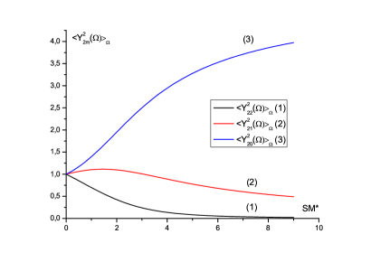
Figure 3: Dependence of quantities $\langle Y_{2m}^{2}(\Omega)\rangle_{\Omega}$ on parameter $SM^{*}$ for $m=0,1,2$.

4.2 Correction to the single-particle distribution function

Correction to the single-particle distribution function due to Gaussian fluctuations can be found according to

$$\frac{\rho^{\rm CR}(\Omega)}{\rho} =\frac{f^{\rm MF}(\Omega)}{Z^{\prime}}\big{(}1+[h(r,\Omega_{1}\Omega_{2})-C(r,\Omega_{1}\Omega_{2})]\big{)}\left|{}_{\begin{smallmatrix}\Omega_{1}\rightarrow\Omega_{2}\\ \mathbf{r}_{1}\rightarrow\mathbf{r}_{2}\end{smallmatrix}}\right.$$

$$=\frac{1}{Z^{\prime}}\,\re^{\,\frac{3}{2}M^{*}S\cos^{2}\theta}\big{(}1+\sum\limits_{m}Y_{2m}^{*}(\Omega)Y_{2m}(\Omega)[h_{22m}(r)+\beta\nu(r)]\big{)}\bigg{|}_{r\rightarrow 0},$$ (31)

where the normalization constant $Z^{\prime}$ can be found from condition $\int\rho^{\rm CR}(\Omega)\rd\Omega=\rho$. Since

$$\lim_{r\rightarrow 0}[h_{22m}(r)+\beta\nu(r)]=-\frac{1}{5}\beta^{*}\left[\sqrt{1-\frac{1}{5}\langle Y_{2m}^{2}(\Omega)\rangle_{\Omega}M^{*}}-1\right],$$ (32)

then the corrected single-particle distribution function has the form

$$\frac{\rho^{\rm CR}(\Omega)}{\rho}=\frac{\re^{\frac{3}{2}SM^{*}\cos^{2}\theta}\left(1+\beta^{*}-\frac{1}{5}\beta^{*}\sum\limits_{m}|Y_{2m}(\Omega)|^{2}\,\sqrt{1-\frac{1}{5}\langle Y_{2m}^{2}(\Omega)\rangle_{\Omega}M^{*}}\right)}{\int\rd\Omega\,\re^{\frac{3}{2}M^{*}S\cos^{2}\theta}\left(1+\beta^{*}-\frac{1}{5}\beta^{*}\sum\limits_{m}|Y_{2m}(\Omega)|^{2}\,\sqrt{1-\frac{1}{5}\langle Y_{2m}^{2}(\Omega)\rangle_{\Omega}M^{*}}\right)}\,.$$ (33)

We can also approximate the corrected single-particle distribution function in an exponential form as

$$\frac{\rho^{\rm EXP}(\Omega)}{\rho}=\frac{1}{Z^{\prime\prime}}\exp\left[\frac{3}{2}M^{*}S\cos^{2}\theta-\frac{1}{5}\beta^{*}\sum\limits_{m}|Y_{2m}(\Omega)|^{2}\,\sqrt{1-\frac{1}{5}\langle Y_{2m}^{2}(\Omega)\rangle_{\Omega}M^{*}}\right],$$ (34)

where $Z^{\prime\prime}$ is the normalization constant such that $\int\rho^{\rm EXP}(\Omega)\rd\Omega=\rho$.

Note that

$$|Y_{2m}(\Omega)|^{2}=\sum\limits_{l}\frac{5}{(2l+1)^{\frac{1}{2}}}\left(\begin{array}[]{ccc}{\,2}\quad\,{\,\,2}\quad{\,l}\\ {m}\,\,{-m}\,\,{\,\,0}\end{array}\right)\left(\begin{array}[]{ccc}{2}\quad{2}\quad{l}\\ {0}\quad{0}\quad{0}\end{array}\right)Y_{l0}(\Omega),$$ (39)

where $l=0,2,4$; $\left(\begin{smallmatrix}2&2&l\\ m&-m&0\end{smallmatrix}\right)$ and $\left(\begin{smallmatrix}2&2&l\\ 0&0&0\end{smallmatrix}\right)$ are the corresponding Clebsch-Gordon coefficients [17].

We can see that in the Gaussian approximation the dependence of the single-particle distribution function on $\beta^{*}$ and $\rho^{*}$ is more complicated than in the MFA: $\rho(\Omega)$ now depends not only on $M^{*}$ but there is also a direct $\beta^{*}$-dependence and a $\langle Y_{2m}^{2}(\Omega)\rangle_{\Omega}$-dependence. We also see that in the Gaussian approximation the single-particle distribution function contains Legendre polynomials of the second and fourth orders of molecule orientations whereas in the linear approximation only Legendre polynomials of the second order are present. From expression (34) it is readily seen that the role of the fluctuation term increases with an increase of inverse temperature $\beta^{*}$.

4.3 Free energy, pressure, and chemical potential

For a homogeneous system, the part of the Helmholtz free energy responsible for field interaction can be calculated by integrating with respect to the coupling parameter $\lambda$:

$$F-F_{\rm id}=\frac{V}{2}\int\rd\mathbf{r}\rd\Omega_{1}\rd\Omega_{2}\rho(\Omega_{1})\rho(\Omega_{2})\nu(r,\Omega_{1}\Omega_{2})\int\limits_{0}^{1}\rd\lambda[1+h(\lambda,r,\Omega_{1}\Omega_{2})],$$ (40)

where

$$h(\lambda,r,\Omega_{1}\Omega_{2}) =\sum\limits_{m}h_{2m}(\lambda,r)Y^{*}_{2m}(\Omega_{1})Y_{2m}(\Omega_{2})$$

$$=\sum\limits_{m}\left(-\frac{\lambda\beta{A}}{r}\frac{1}{5}\exp\left[-r\sqrt{{\alpha^{2}+\langle{Y_{2m}^{2}(\Omega)}\rangle_{\Omega}{\frac{1}{5}4\pi\rho\beta{A}\lambda}}}\right]\right)Y_{2m}^{*}(\Omega_{1})Y_{2m}(\Omega_{2}).$$ (41)

Expression (40) in terms of parameter $B=\frac{1}{5}4\pi\rho\beta A$ yields

$$\beta\left(F-F_{\rm id}\right) =V\frac{B\rho}{2\alpha^{2}}\langle Y_{20}(\Omega)\rangle^{2}_{\Omega}$$

$$+V\sum\limits_{m}\left[-\frac{\left(\alpha^{2}+\langle Y_{2m}^{2}(\Omega)\rangle_{\Omega}B\right)^{3/2}}{12\pi}+\frac{\alpha^{3}}{12\pi}+\frac{\alpha\langle{Y_{2m}^{2}(\Omega)}\rangle_{\Omega}B}{8\pi}\right].$$ (42)

Having an explicit expression for the free energy, we can find the pressure:

$$\beta P= -\beta\left[\frac{\partial}{\partial V}F\right]_{T,N}=\rho+\frac{B\rho}{2\alpha^{2}}\left(\langle Y_{20}(\Omega)\rangle^{2}_{\Omega}+\rho\frac{\partial}{\partial\rho}\langle Y_{20}(\Omega)\rangle^{2}_{\Omega}\right)$$

$$-\sum\limits_{m}\left(-\frac{\left(\alpha^{2}+\langle Y_{2m}^{2}(\Omega)\rangle_{\Omega}B\right)^{3/2}}{12\pi}+\frac{\alpha^{3}}{12\pi}+\frac{\alpha\langle{Y_{2m}^{2}(\Omega)}\rangle_{\Omega}B}{8\pi}\right)$$

$$+\frac{\rho B}{8\pi}\sum\limits_{m}\left(\frac{1}{\rho}\langle Y_{2m}^{2}(\Omega)\rangle_{\Omega}+\frac{\partial}{\partial\rho}\langle Y_{2m}^{2}(\Omega)\rangle_{\Omega}\right)\left(\alpha-\left(\alpha^{2}+\langle Y_{2m}^{2}(\Omega)\rangle_{\Omega}B\right)^{1/2}\right),$$ (43)

where the derivatives of the averages $\langle\ldots\rangle_{\Omega}$ are equal to

$$\frac{\partial}{\partial\rho}\left\langle Y_{2m}^{2}(\Omega)\right\rangle_{\Omega} =\frac{B}{\rho\alpha^{2}}\left(\left\langle Y_{20}(\Omega)\right\rangle_{\Omega}+\rho\frac{\partial}{\partial\rho}\left\langle Y_{20}(\Omega)\right\rangle_{\Omega}\right)$$

$$\times\bigg{(}\left\langle Y_{2m}^{2}(\Omega)\right\rangle_{\Omega}\left\langle Y_{20}(\Omega)\right\rangle_{\Omega}-\left\langle Y_{2m}^{2}(\Omega)Y_{20}(\Omega)\right\rangle_{\Omega}\bigg{)},$$ (44)

$$\frac{\partial}{\partial\rho}\left\langle Y_{20}(\Omega)\right\rangle_{\Omega} =\frac{B\left[\left\langle Y_{20}(\Omega)\right\rangle_{\Omega}^{3}-\left\langle Y_{20}^{2}(\Omega)\right\rangle_{\Omega}\left\langle Y_{20}(\Omega)\right\rangle_{\Omega}\right]}{\rho\alpha^{2}-\rho B\left[\left\langle Y_{20}(\Omega)\right\rangle^{2}_{\Omega}-\left\langle Y_{20}^{2}(\Omega)\right\rangle_{\Omega}\right]}\,.$$ (45)

In the isotropic phase $\langle Y_{20}(\Omega)\rangle_{\Omega}=0$ and expression (4.3) considerably simplifies:

$$\beta P =-\beta\left[\frac{\partial}{\partial V}F\right]_{T,N}=\rho+\sum\limits_{m}\left(\frac{\alpha^{2}\left(\alpha^{2}+B_{2m}\right)^{1/2}}{12\pi}-\frac{\alpha^{3}}{12\pi}-\frac{B_{2m}\left(\alpha^{2}+B_{2m}\right)^{1/2}}{24\pi}\right),$$ (46)

where $B_{2m}\equiv\langle Y_{2m}^{2}(\Omega)\rangle_{\Omega}B$. This expression is similar to the one obtained in [20, 13], where there is a supplementary summation over $m$ and the quantity $B$ is replaced by $B_{2m}$ . The chemical potential $\mu$ of the fluid can be found from expressions (4.3) and (4.3) as $\mu=\left(F+PV\right)/N$ and equals

$$\beta\mu =\ln\left(\rho\Lambda_{\rm T}^{3}\Lambda_{\rm R}\right)+\frac{B}{\alpha^{2}}\left(\langle{Y_{20}(\Omega)}\rangle^{2}_{\Omega}+\frac{1}{2}\rho\frac{\partial}{\partial\rho}\,\langle{Y_{20}(\Omega)}\rangle^{2}_{\Omega}\right)$$

$$+\frac{B}{8\pi}\sum\limits_{m}\left(\frac{1}{\rho}\langle Y_{2m}^{2}(\Omega)\rangle_{\Omega}+\frac{\partial}{\partial\rho}\langle Y_{2m}^{2}(\Omega)\rangle_{\Omega}\right)\left(\alpha-\left(\alpha^{2}+\langle Y_{2m}^{2}(\Omega)\rangle_{\Omega}B\right)^{1/2}\right).$$ (47)

4.4 Broken symmetry problem and the elasticity constant

A specific feature of the considered molecular fluid is a broken symmetry which appears in the absence of an orienting external field. In [2, 3, 7] using the Lovett-Mou-Buff-Wertheim equation [21, 22] an exact relation for orientationally non-uniform fluids was obtained:

$$\boldsymbol{\nabla}_{\Omega_{1}}\ln\rho(\Omega_{1})=\int\rd\mathbf{r}_{12}\rd\Omega_{2}C(\mathbf{r}_{12}\,,\Omega_{1}\Omega_{2})\boldsymbol{\nabla}_{\Omega_{2}}\rho(\Omega_{2}),$$ (48)

where $C(\mathbf{r}_{12}\,,\Omega_{1}\Omega_{2})$ is the direct correlation function which in the RPA is given by equation (24).

Equation (48) is also known as the integro-differential form of the Ward identity [2, 7, 23]. The angular gradient operator $\boldsymbol{\nabla}_{\Omega}$ decomposes into 3 spherical components ${\nabla}_{0}$ , ${\nabla}_{+}$ , ${\nabla}_{-}$ . As ${\nabla}_{0}$ is oriented in the direction of liquid crystal, it vanishes due to rotational invariance. For other components, the following relations hold [17]:

$$\nabla_{\pm}Y_{lm}(\Omega)=\left[l(l+1)-m(m\pm 1)\right]^{1/2}Y_{l,m\pm 1}\,.$$ (49)

The direct correlation function can be expanded as [2]

$$C(r_{12}\,,\Omega_{1}\Omega_{2})=\sum\limits_{lml^{\prime}m^{\prime}}C_{lml^{\prime}m^{\prime}}(r_{12})Y_{lm}^{*}(\Omega_{1})Y_{l^{\prime}m^{\prime}}(\Omega_{2}).$$ (50)

Due to the axial symmetry of a nematic, $m=m^{\prime}$. From (48) we derive the following relation for the average $\langle Y_{21}^{2}(\Omega)\rangle_{\Omega}$ :

$$C_{221}\rho\langle Y_{21}^{2}(\Omega)\rangle_{\Omega}=1,$$ (51)

where

$$C_{221}=\int\rd\mathbf{r}_{12}C_{221}(r_{12})=-\frac{1}{5}\frac{4\pi\beta A}{\alpha^{2}}\,.$$ (52)

Due to condition (51), harmonic $h_{221}(k)$ diverges in the limit $\mathbf{k}\rightarrow 0$ signalling the appearance of Goldstone modes in the system. This phenomenon is responsible for a number of unique properties of nematics such as elastic behavior and critical light scattering. The other harmonics of the pair correlation function should be finite according to the phenomenological theory of de Gennes [15]. In the considered approximation (24) we have

$$C_{220}=C_{221}=C_{222}$$ (53)

and due to (51) and (52)

$$\left(\alpha^{2}+\frac{1}{5}4\pi\rho\beta A\left\langle Y_{2m}^{2}(\Omega)\right\rangle_{\Omega}\right)^{1/2}=\alpha\left(1-\frac{\left\langle Y_{2m}^{2}(\Omega)\right\rangle_{\Omega}}{\left\langle Y_{21}^{2}(\Omega)\right\rangle_{\Omega}}\right)^{1/2}.$$ (54)

As we can see from figure 3, for $m=2$, the ratio $\left\langle Y_{22}^{2}(\Omega)\right\rangle_{\Omega}/\left\langle Y_{21}^{2}(\Omega)\right\rangle_{\Omega}<1$ and $h_{222}(r)$ is well defined. However, for $m=0$, the ratio $\left\langle Y_{20}^{2}(\Omega)\right\rangle_{\Omega}/\left\langle Y_{21}^{2}(\Omega)\right\rangle_{\Omega}>1$ and $h_{220}(r)$ is not defined. For this reason, a problem arises also for thermodynamic properties and for the density correction. This problem is connected with approximation (24) which leads to (53). We should mention that in previous works [2, 3, 7] carried out in the mean spherical approximation equation (53) is not true and the problem being discussed does not appear. We think that for point particles we can also solve this problem by introducing an additional isotropic interaction. We will consider this aspect of the problem in a separate paper.

Broken symmetry is connected with elasticity properties of the considered fluid which are described by the elasticity constant $K$. Formal expression for $K$ as proposed by Poniewiersky and Stecki [24] within our model reads

$$\beta K =\frac{1}{6}\int\rd\mathbf{r}\rd\Omega_{1}\rd\Omega_{2}r^{2}\frac{\partial\rho(\Omega_{1})}{\partial\cos\theta_{1}}\frac{\partial\rho(\Omega_{2})}{\partial\cos\theta_{2}}n_{x}(\Omega_{1})n_{x}(\Omega_{2})C(r,\Omega_{1}\Omega_{2})$$

$$=10\pi\rho^{2}S^{2}\int r^{4}C_{221}(r)\rd r=-12\pi\rho^{2}S^{2}\frac{\beta A}{\alpha^{4}}\,.$$ (55)

Another way to calculate elastic constants comes from the theory of hydrodynamic fluctuations [24] and can be found as

$$\beta K=3\left[\lim\limits_{k\rightarrow 0}k^{2}h_{221}(k)\frac{\langle Y^{2}_{21}(\Omega)\rangle^{2}_{\Omega}}{\langle Y_{20}(\Omega)\rangle^{2}_{\Omega}}\right]^{-1}=-12\pi\rho^{2}S^{2}\frac{\beta A}{\alpha^{4}}\,.$$ (56)

As we see, both expressions for $K$ are identical.

Figure 4: Temperature dependence of the elasticity constant.

Figure 5: Density dependence of the elasticity constant.

Dependencies of the reduced elasticity constant $K^{*}=-K/A\alpha^{2}=12\pi S^{2}\rho^{*2}$ on temperature $T^{*}$ and density $\rho^{*}$ are presented in figures 4.4 and 4.4. One can see that with increasing temperature the elasticity constant decreases and with increasing density it increases. The effect is more pronounced respectively for larger density and for larger temperature. This result is in agreement with the previous result [7] obtained in the framework of the mean spherical approximation for a non-point model of the nematogenic Maier-Saupe fluid.

5 Conclusions

In this paper, for the first time the field theoretical approach is applied to the description of correlation functions and thermodynamic properties of molecular anisotropic fluids. As an example we consider a Maier-Saupe nematogenic fluid with the Yukawa potential of interparticle interaction. By expanding the Hamiltonian in powers of density fluctuations we examine the system in the mean field and Gaussian approximations.

In the mean field approximation, we obtain analytical expressions for the single-particle distribution function and the orientational order parameter which are in agreement with the classical Maier-Saupe theory for nematic ordered fluids.

In the Gaussian approximation we find analytical expressions for the pair correlation function, the free energy, the pressure, the chemical potential, and the elasticity constant. We calculate the correction to the mean field single-particle distribution function due to fluctuations and show that the corrected single-particle distribution function has a more complex dependence on density and temperature compared to the MFA. In contrast to the MFA single-particle distribution function, it includes the fourth order Legendre polynomials of molecule orientations in addition to the second order ones. We also use Ward symmetry identity to derive a simple expression for the average of spherical harmonic $\left\langle Y_{21}^{2}(\Omega)\right\rangle$. One consequence of this condition is that for the system to be stable, the distance-dependent part of the interaction should be attractive. We show that in the Gaussian approximation the harmonic $h_{221}(k)$ diverges in the limit $\mathbf{k}\rightarrow 0$. Such a situation occurs at the phase transition from an isotropic to a nematic phase. This change in symmetry causes collective fluctuations known as the Goldstone modes. However, in the RPA for the considered system, the harmonic $h_{220}(k)$ is not defined. We hope to solve this problem in our next paper by introducing additional isotropic interparticle interactions.

Нематичний плин Майєра-Заупе: теоретико-польовий пiдхiд М. Головкоlabel1, Д. дi Капрiоlabel2, I. Кравцiвlabel1 label1 Iнститут фiзики конденсованих систем НАН України, вул. I. Свєнцiцького, 1, 79011 Львiв, Україна label2 Лабораторiя електрохiмiї, хiмiї поверхонь i енергетичного моделювання, Вiддiлення хiмiї вищої нацiональної школи ПарiТех, пл. Жуссю, 4, 75005 Париж, Францiя

References

[1] Maier W., Saupe A., Z. Naturforsch., A: Phys.
Sci., 1959, 14, 882;
ibid., 1960, 15, 287.
[15] de Gennes P.G., The Physics of Liquid Crystals.
Oxford University Press, Oxford, 1974.
[16] Holovko M., Concept of ion association in the
theory of electrolyte solutions. – In: Ionic soft matter:
Modern trends in theory and applications. NATO Science Series, 2005, 206, 45,
eds. Henderson D., Holovko M., Trokhymchuk A., Springer, Berlin;
doi:10.1007/1-4020-3659-0_3.
[17] Gray C.G., Gubbins K.E., Theory of Molecular
Fluids. Clarendon press, Oxford, 1984.
[18] Yukhnovsky I.R., Holovko M.F., The
Statistical Theory of Classical Equilibrium Systems.
Naukova Dumka, Kyiv, 1980 (in Russian).
[19] Hansen J.P., McDonald I.R., Theory of Simple
Liquids. Academic Press, Oxford, 2004.
[20] Holovko M., Kravtsiv I., Soviak E.,
Condens. Matter Phys., 2009, 12, 137.
[21] Lovett R., Mou C.Y., Buff F.P.,
J. Chem. Phys., 1976, 65, 570; doi:10.1063/1.433110.
[22] Wertheim M., J. Chem. Phys., 1976, 65,
2377; doi:10.1063/1.433352.
[23] di Caprio D., Zhang Q., Badiali J.P., Phys. Rev.
E, 1996, 53, 2320; doi:10.1103/PhysRevE.53.2320.