Straightforward quantum-mechanical derivation of the
Crooks fluctuation theorem and the Jarzynski equality

Abstract

We obtain the Crooks and the Jarzynski non-equilibrium fluctuation relations using a direct quantum-mechanical approach for a finite system that is either isolated or coupled not too strongly to a heat bath. These results were hitherto derived mostly in the classical limit. The two main ingredients in the picture are the time-reversal symmetry and the application of the first law to the case where an agent performs work on the system. No further assumptions regarding stochastic or Markovian behavior are necessary, neither a master equation or a classical phase-space picture are required. The simplicity and the generality of these non-equilibrium relations are demonstrated, giving very simple insights into the Physics.

I Introduction

In contrast to the situation in equilibrium statistical physics, and linear response theory, there are not so many well-established results for systems far from equilibrium NFT1 ; NFT2 ; NFT3 . Two such extremely interesting results are the “nonequilibrium fluctuation theorem” (NFT) of Crooks Crooks and the related Jarzynski equality Jarzynski ; VB . Both have to do with the work done by/on a finite system coupled to a heat bath. We also mention here previous works rsp ; Gavish ; book , showing that the Kubo formalism, the fluctuation-dissipation theorem, and the associated detailed-balance relations are valid in a large class of nonequilibrium steady-state systems, and not only in equilibrium.

The system under consideration is described by a time dependent Hamiltonian ${\cal H}(X(t))$, where the parameter $X$ is a time-dependent c-number, often coupled linearly to an observable of the system. At ${t=t_{0}}$ the system is prepared in thermal equilibrium at the temperature $T$. The thermalization is achieved by connecting it for a long enough time to a thermal bath at that temperature. After that, within the time ${t=t_{1}}$, the system undergoes a “work process”. This means that an “agent” changes the value of $X$ from $X_{0}$ to $X_{1}$. During this process a work $\mathcal{W}$ is performed on the system, and possibly some heat $\mathcal{Q}$ is dissipated into the bath LL . In the simplest scenario the system is isolated, and heat flow is not involved. It should be emphasized that at the end of the work process, the system is in general not in equilibrium.

The NFT deals with the probability distribution $P(\mathcal{W})$ of the work $\mathcal{W}$, whose experimental determination requires to repeat the process protocol many times, and to record the measured values of $\mathcal{W}$. Specifically the NFT concerns the ratio $P_{0\leadsto 1}(\mathcal{W})/P_{1\leadsto 0}(-\mathcal{W})$ between the statistics of the forward scenario, and the statistics of the reversed scenario. In the latter, the system is equilibrated with the same bath under conditions such that ${X=X_{1}}$. Then the time-reversed process protocol is realized, such that at the final time ${X=X_{0}}$.

Derivations of various quantum mechanical versions of the NFT have been discussed in several publications q1 ; q2 ; q3 ; NFTx ; hanggi ; CrooksJQ ; VV . However, a major subtlety arises with regard to the definition of work. Citing the introduction of Ref.CrooksJQ : “The generalization of the Jarzynski identity to closed system quantum dynamics is technically straightforward […] However, for a system that can interact with the environment this does not suffice […] Unlike for a classical system, we cannot continuously measure the energy of the system without severely disturbing the dynamics of the system”.

The objective of our paper is to present a simple derivation of the NFT in the quantum mechanical context, bypassing various subtleties that, in our view, have obscured the simple physics involved. The main issue is to define carefully the notion of work in the quantum mechanical context, and to clarify the role that is played by the bath.

Outline: We refer to the evolution during a work process, and formulate for it a generalized detailed balance relation. Then we discuss the notion of work, leading to the NFT of Crooks. The main issue is the modeling the work agent, and the understanding of the role that is played by the bath. The implied Jarzynski equality and the implications on the dissipated work and on the entropy production are briefly discussed.

II Evolution during a work process

The system under consideration is described by a time-dependent Hamiltonian ${\cal H}(X(t))$. Let us assume that a classical “agent” changes the value of the c-number control parameter $X$ from $X_{0}$ at ${t=t_{0}}$ to $X_{1}$ at ${t=t_{1}}$. In some cases, but not in general, the actual duration of the time dependent stage might be ${\tau\ll|t_{1}-t_{0}|}$. Given that at ${t=t_{0}}$ the system has been prepared in some eigenstate $n^{(0)}$ of ${\cal H}(X_{0})$, we ask what is the probability $\mathrm{P}_{0\leadsto 1}(m|n)$ that at the later time ${t=t_{1}}$ it is measured in an eigenstate $m^{(1)}$ of ${\cal H}(X_{1})$. Below we use the notation

$$\omega\ \ =\ \ E_{m}^{(1)}-E_{n}^{(0)}$$ (1)

In a later section we shall define the notion of work $\mathcal{W}$, and shall explain that up to some uncertainty, we can make the identification ${\mathcal{W}=\omega}$, provided the system is isolated from the environment.

For a strict quantum adiabatic process one has $\mathrm{P}(m|n)=\delta_{n,m}$. But we are interested in more general circumstances. In particular we focus in this section on unitary evolution for which

$$\mathrm{P}_{0\leadsto 1}(m|n)\ \ =\ \ \Big{|}\langle m^{(1)}|U_{0\leadsto 1}|n^{(0)}\rangle\Big{|}^{2},$$ (2)

where $U$ is the time-evolution operator. What is important for the derivation of the NFT is the micro-reversibility of the dynamics, namely,

$$\mathrm{P}_{1\leadsto 0}(n|m)\ \ =\ \ \mathrm{P}_{0\leadsto 1}(m|n)$$ (3)

Note that in general the reversed process requires to transform some fields, e.g. to change the sign of the magnetic field if present.

For completeness it is also useful to define the notion of “classical dynamics”. Given phase-space, we can divide it into cells with some arbitrary desired resolution. Then we can regard $n$ as an index that labels cells in phase space. The classical equations define a map

$$|n^{(1)}_{final}\rangle\ \ =\ \ \mathsf{M}\ |n^{(0)}_{initial}\rangle$$ (4)

We use quantum style notations in order to make the relation to the quantum formulation clear. It follows that $\mathrm{P}(m|n)$, instead of being a stochastic kernel, becomes a deterministic kernel that induces permutations

$$\mathrm{P}_{0\leadsto 1}(m|n)\Big{|}_{classical}\ \ =\ \ \delta_{m,\mathsf{M}n}$$ (5)

The derivation in the next section does not depend on whether the dynamics is “classical” or “stochastic” or “quantum” in nature as long as the measure and the micro-reversibility are preserved. The preservation of measure is reflected by our discrete notations: If, say, we had deterministic dynamics that does not satisfy Liouville theorem, we could not have used the above “cell construction”

III The generalized detailed balance relation

The power spectrum of the fluctuations of an observable $A$ is given by the following spectral decomposition

$$\tilde{S}(\omega)\ \ =\ \ \sum_{n,m}p_{n}\ \Big{|}\langle m|A|n\rangle\Big{|}^{2}\ \delta\Big{(}\omega-(E_{m}-E_{n})\Big{)}$$ (6)

Here we assume a time independent Hamiltonian, and stationary preparation that can be regarded as a mixture of eigenstates with weights $p_{n}$. For a canonical preparation

$$p_{n}\ \ =\ \ \frac{1}{Z}\mbox{e}^{-E_{n}/T}\ \ =\ \ \exp\left[-\frac{E_{n}-F(X_{0})}{T}\right]$$ (7)

where $Z$ is the partition function, and $F(X)$ is the Helmholtz free energy at temperature $T$, calculated here for the fixed value of the control parameter $X$. Then one obtains after two lines of straightforward algebra, the detailed balance relation

$$\frac{\tilde{S}(\omega)}{\tilde{S}(-\omega)}\ \ =\ \ \exp\left[\frac{\omega}{T}\right]$$ (8)

This relation plays a key role in the linear response theory. Specifically it reflects the ratio between the tendency of the system to absorb and emit energy from/to a driving source $-f(t)A$.

In complete analogy we define the following spectral kernel:

$$P_{0\leadsto 1}(\omega)$$ (9)

$$\ \ =\sum_{n,m}p_{n}^{(0)}\ \mathrm{P}_{0\leadsto 1}(m|n)\ \delta\Big{(}\omega-(E_{m}^{(1)}-E_{n}^{(0)})\Big{)}$$

Here the superscript indicates whether we refer to the initial Hamiltonian $\mathcal{H}(X_{0})$ or to the final Hamiltonian $\mathcal{H}(X_{1})$. For the reversed process we write

$$P_{1\leadsto 0}(\omega)$$ (10)

$$\ \ =\sum_{m,n}p_{m}^{(1)}\ \mathrm{P}_{1\leadsto 0}(n|m)\ \delta\Big{(}\omega-(E_{n}^{(1)}-E_{m}^{(0)})\Big{)}$$

It immediately follows, in analogy with the usual detailed balance condition, that the ratio of the spectral functions $P_{0\leadsto 1}(\omega)$ and $P_{1\leadsto 0}(-\omega)$ is determined by the ratio of the initial probabilities $p_{n}^{(0)}$ and $p_{n}^{(1)}$, leading to

$$\frac{P_{0\leadsto 1}(\omega)}{P_{1\leadsto 0}(-\omega)}\ \ =\ \ \exp\left[\frac{\omega-(F(X_{1})-F(X_{0}))}{T}\right],$$ (11)

where both $F(X_{1})$ and $F(X_{0})$ refer to the same preparation temperature $T$. Note again that if $X$ does not change in time, this relation formally coincides with the detailed balance relation Eq.​​ (8).

IV The notion of work and the NFT of Crooks

The main difficulty in the quantum formulation of the NFT concerns the definition of work hanggi ; CrooksJQ ; w0 ; w1 ; w2 . Consider first an isolated system. Naively we can define ${\mathcal{W}=\omega}$, namely the work is the change in the energy of the system. But in the quantum reality this means that we have to do a measurement of the initial stage, hence the state of the system collapses and it is no longer canonical.

Furthermore, assume that we want to consider a multi-stage process that extends over two time intervals ${t_{0}\rightarrow t_{1}\rightarrow t_{2}}$. We would like to say that the work done is the sum $\mathcal{W}_{0\leadsto 1}+\mathcal{W}_{1\leadsto 2}$. With the above definition we have to perform a measurement at the time instant $t_{1}$. But in the quantum mechanical reality we might not have the time for that (see further discussion below).

It is therefore clear that the definition of work requires refinement. One possible direction hanggi is to define

$$\mathcal{W}_{0\leadsto 1}=\int_{t_{0}}^{t_{1}}\frac{\partial\mathcal{H}}{\partial X}\dot{X}dt$$ (12)

Then, in analogy with the theory of counting statistics levitov ; nazarov ; cnz , one might say that a continuous measurement is required, involving a weak coupling to a von Neumann pointer. The problem with this approach is that the counting statistics quasi probability nazarov ; cnz has no simple physical interpretation, and might be even negative.

It turns out that in the present context there is a simple way out of these subtleties, that parallels the conventional classical perspective w0 . Instead of regarding $X(t)$ as a c-number field, we regard it as a dynamical variable of an “agent” that is doing work. The total Hamiltonian can be formally written as

$$\mathcal{H}_{\mbox{\tiny total}}\ \ =\ \ \mathcal{H}(r;X)+\mathcal{H}_{agent}(X)$$ (13)

where $r$ stands for system dynamical variables, and $X$ is the agent degree of freedom. Then we define the work $\mathcal{W}$ as the change in the energy of the agent

$$\mathcal{W}\ \ =\ \ E_{agent}(0)-\mathcal{H}_{agent}$$ (14)

where $E_{agent}(0)$ is its initial energy, which is assumed to be well defined up to some small uncertainty.

It should be clear that by treating the agent as a dynamical variable we bypass the energy-time uncertainty fallacy, as discussed long ago AB . Once the energy is transferred to an agent, there is no theoretical limitation on the accuracy of its measurement, irrespective of the time-of-measurement issue.

In our treatment it is assumed that we have control over the strength of the interaction between the system and the agent. Hence we have the option to switch “on” the interaction in two possible ways:  (i) within a restricted region in ${(r,X)}$ space;  (ii) within a restricted time duration. In the latter case the Hamiltonian Eq.​​ (13) would become time dependent, and consequently we would not have control over the precise $X$ displacement of the agent.

Once the notion of work is clarified it follows automatically that for an isolated system $\mathcal{W}=\omega$, to the extent that the unavoidable quantum uncertainties can be ignored. From here follows the Crooks relation

$$\frac{P_{0\leadsto 1}(\mathcal{W})}{P_{1\leadsto 0}(-\mathcal{W})}\ \ =\ \ \exp\left[\frac{\mathcal{W}-(F(X_{1})-F(X_{0}))}{T}\right]$$ (15)

Instead of going on with an abstract discussion of what do we mean by “work agent”, we consider below two simple prototype models that illuminate this notion.

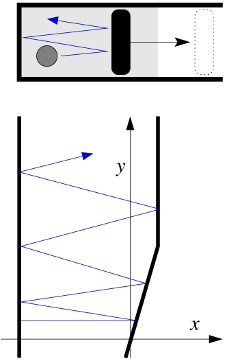
Figure 1: The system is a gas of particles in a box. The box region is indicated by grey. A representative trajectory is illustrated. The “agent” on which work is being done is a piston that is free to move to infinity. After the piston is pushed out the gas particles stay in the box, and no longer interact with the piston, but possibly may interact (say) with a bath or with other agents. At the end of each single ”run” of the experiment, there is an unlimited time to measure the energy of the freely moving piston in the desired resolution.

V Modeling the work agent

In order to define the notion of work we find it essential to regard the “agent” as a dynamical entity. It can be another object (“piston”) from/to which energy is transferred, or it can be a field with which the system interacts, absorbing or emitting excitations (“photons”).

V.1 Modeling the agent as a piston

The prototype model for explaining the notion of work in standard thermodynamics textbooks is the gas-piston system that is illustrated in Fig.​​ 1. The “agent” on which work is being done is a piston that is free to move to infinity. After the piston is pushed out the gas particles stay in the box, and no longer interact with the piston, but possibly may interact (say) with a bath or with other agents as in Fig.​​ 2. At the end of each single ”run” of the experiment, there is an unlimited time to measure the energy of the freely moving piston in the desired resolution.

The essential ingredient in the illustrated construction is the decoupling at the end of the interaction: After the piston moves outside of the shaded region, it becomes a free object whose kinetic energy we can measured without having a time limitation.

For presentation purposes, but without any loss of generality, we consider a single gas particle and regard the box as one dimensional. The Hamiltonian is

$$\mathcal{H}_{\mbox{\tiny total}}(r,p;X,P)=\frac{p^{2}}{2\mathsf{m}}+V_{\mbox{\tiny box}}(r)+u(r{-}X)+\frac{P^{2}}{2M}$$ (16)

where $u(r-X)=u_{0}\delta(r-X)$ with ${u_{0}=\infty}$. Thanks to a potential $V_{\mbox{\tiny box}}$ the gas particle remains in the shaded region even if the piston is “out”. Once the piston is out the “system” no longer affects the “agent”, nor affected by it.

In order to visualize the dynamics it is convenient to define $\alpha=(\mathsf{m}/M)^{1/2}$, and ${p_{x}=p}$, and ${p_{y}=\alpha P}$, and ${x=r}$, and ${y=(1/\alpha)X}$. Then the Hamiltonian takes the form

$$\mathcal{H}_{\mbox{\tiny total}}=\frac{1}{2\mathsf{m}}(p_{x}^{2}+p_{y}^{2})+V_{\mbox{\tiny box}}(x)+u(x-\alpha y)$$ (17)

We assume that initially the piston is prepared in rest with some uncertainty $\Delta X$ in its position, and an associated uncertainty ${\Delta P\sim 1/\Delta X}$ in its momentum. Accordingly the uncertainty of the total energy is

$$\Delta E\ \ \sim\ \ [M\Delta X^{2}]^{-1}+\Delta E_{\mbox{\tiny system}}$$ (18)

The total energy $E$ is a constant of motion. It follows that the probability distribution of the total energy is a $\delta$ function. The total energy $E$ is the sum of the particle energy and the piston energy. Let us denote the increase in the particle energy as $\omega$, and the decrease in the piston energy as $\mathcal{W}$. It follows that the joint distribution is

$$\mathrm{P}(\omega,\mathcal{W})\ \ =\ \ P(\omega)\ \delta(\mathcal{W}-\omega)$$ (19)

where the equality is justified to the extent that $\Delta E$ can be neglected. Under such conditions the distribution of work $P(\mathcal{W})$ is the same as $P(\omega)$.

The argument above has established the equality of $P(\mathcal{W})$ and $P(\omega)$ for a system that is prepared in a microcanonical state, such that $\Delta E_{\mbox{\tiny system}}$ is a small uncertainty. But trivially the equality of the two distributions extends to any mixture, and in particular to the canonical preparation under consideration. We note that our definition of $P(\omega)$ in the previous section has assumed a c-number driving source, while here there is some uncertainty $\Delta X$ in the position of the piston. Accordingly a trade-off is required with regard to $\Delta X$ and $\Delta E$. This trade-off is the physical limit of the NFT applicability. In practice, and in particular for large deviations, this uncertainty should not be an issue.

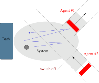
Figure 2: (color online) Illustration of a multi-stage process that consists of time intervals during which the system interacts with a bath, and with two different agents. The system is a gas particles that are confined to move in the shaded area. The interaction with the first agent is as described in Fig.​​ 1. The second agent compresses that gas, until the interaction with it is switched off: then it becomes like a free particle.

V.2 Modeling the agent as a field

In this subsection we consider another illuminating example for a “work agent” but with a different emphasis: we would like to illuminate the role that is played by the strength of the system-agent interaction. For this purpose the piston model is somewhat unnatural because perturbation theory is not well controlled. This is the motivation to consider a different example. Below the agent is a field with which the system interacts, and the measurement is the detection of a field quanta. These quanta can be observed at any later time without disturbing the on-going driving cycle.

For sake of clarity the reasoning below is based on the traditional weak coupling assumption. Namely, we assume that the driving induces transitions that are determined by the Fermi-Golden-Rule. While we employed below perturbation-theory thinking, we re-emphasize that these considerations are much more general: for stronger perturbations, one may think in terms of the evolution operator $U$ of Eq.​​ (2), and microscopic reversibility Eq.​​ (3) follows mutatis mutandis.

Consider a classical force $\mathcal{F}$ that arises, say, from a classical electric field that acts on charged particles. Taking the coupling to be via the total dipole moment of the system, the interaction term is

$$\mathcal{H}_{\mbox{\tiny system-agent}}\ \ =\ \ -\mathcal{F}(t)\sum r_{i}$$ (20)

where the $r_{i}$ are the coordinates of the particles along the relevant axis, and $\mathcal{F}(t)$ is a c-number force that is switched from ${\mathcal{F}_{0}=0}$ at $t_{0}=0$, to ${\mathcal{F}_{1}=\delta\mathcal{F}}$ at time $t_{1}$.

To see what is going on, think of expanding $\mathcal{F}(t)$ in a Fourier integral. The Fourier components $\mathcal{F}_{\omega}$ are significant on an interval of order $1/\tau$, where $\tau$ is the actual duration of the variation, which is possibly small compared with ${|t_{1}-t_{0}|}$. Small $\delta\mathcal{F}$ and/or small $\tau$ make the relevant Fourier components small. From low order perturbation theory it follows that the transitions are to levels $E_{m}$ whose energy is within $\sim 1/\tau$ of the initial energy $E_{n}$, with probabilities proportional to $|\mathcal{F}_{\omega}|^{2}$. Very importantly, energy is conserved in the sense that the excitation takes an energy ${\omega=E_{m}-E_{n}}$ from the field. We know that if we quantize the field ${\mathcal{F}}$, a photon with the energy ${\omega=E_{m}-E_{n}}$ will be destroyed during the transition.

A side note is in order: for a closed system, the work done by the classical agent is all converted to a change of the system energy. A well-known even stronger example is that of a probe particle inelastically scattered from the system losing an certain energy which is then equal to the energy of the created excitation(s).

In the absence of a coupling to the bath the transitions are into an energy range ${\Gamma_{F}\approx 1/\tau}$ that may contain many states. When a coupling to the bath is introduced, the levels of the system acquire an additional width $\Gamma_{B}$. If the interaction is weak enough $\Gamma_{B}$ becomes smaller than the mean level spacing of the system.

Before going on with the above reasoning we would like to recall what is the justification for the canonical state. The reader is most probably familiar with the standard textbook argumentation in LL : if a system is weakly coupled to a bath its energy distribution will approach a canonical distribution, as postulated by Gibbs, based on an ergodicity assumption. There is an interesting refined version of this argument that has been introduced by Lipkin . Namely, one can rigorously show that the system would equilibrate to a canonical mixture, with zero off diagonal elements, if $\Gamma_{B}$ is smaller than the mean level spacing of the system. This weak coupling assumption is crucial whenever we try to connect statistical mechanics with thermodynamics, and in particular it is essential for the following argumentation.

Coming back to the work process scenario, it is clear that in order to relate the backward and the forward process we have to assume that the system starts in a canonical mixture state. If the system interacts with a bath it is essential to assume that in the preparation stage, either of the forward or of the reversed process, the system-bath coupling is small enough such that the system eigenstates are not mixed. This is what counts in obtaining Eq.​​ (11). Other than that, energy conservation implies that $\mathcal{W}=\omega$, so again, the distributions of $\omega$ and of $\mathcal{W}$ are the same, hence Eq.​​ (15) follows.

VI The irrelevance of the bath

The Crooks relation and the Jarzynski equality concern the probability distribution of work done during a non-equilibrium process that starts with a canonical state. We deduced in the previous sections that in the case of an isolated system $P(\mathcal{W})$ satisfies the same Crooks relation as $P(\omega)$. We now want to extend the validity of this relation to the case of non-isolated system.

It is clear that the bath is likely to affect significantly the dynamics. In some cases the dissipative dynamics can be described by a Markovian master equation - but we do not want to impose this assumption. Rather, as discussed in last part of section V, we are satisfied with the traditional assumption of small system-bath coupling: it is the same assumption that justifies the emergence of the canonical mixture upon preparation Lipkin . Within the framework of this traditional assumption, let us discuss whether the interaction with the bath can affect the Crooks relation.

First scenario.– After the work process has ended we allow the system to relax to the bath temperature $T$. This additional step does not involve work, as noted in VB , hence $P(\mathcal{W})$ is not affected.

Second scenario.– Assume that there is a finite system-bath coupling $\eta$ during the process. The duration of the process is $\tau$. Inspired by the argumentation of Jarzynski , we regard the system and the bath as one grand-system, for which

$$\frac{P_{0\leadsto 1}(\mathcal{W};\eta,\tau)}{P_{1\leadsto 0}(-\mathcal{W};\eta,\tau)}$$

$$\ \ \ =\exp\left[\frac{\mathcal{W}-(F_{tot}(X_{1};\eta)-F_{tot}(X_{0};\eta))}{T}\right]$$ (21)

It should be clear that $P_{0\leadsto 1}(\mathcal{W})$ and $P_{1\leadsto 0}(-\mathcal{W})$ depend on both $\eta$ and $\tau$. But the ratio, according to Crooks, is independent of $\tau$. Still one suspects that the right-hand side depends on $\eta$. But in fact this is not so. The argument is as follows: The ratio is independent of $\tau$, and therefore we can evaluate it, without loss of generality, for $\tau\rightarrow 0$; But in this ”sudden” limit the result should be independent of $\eta$, because the bath has no time to influence the work. We therefore can set ${\eta=0}$, and deduce that without loss of generality

$$\frac{P_{0\leadsto 1}(\mathcal{W};\eta,\tau)}{P_{1\leadsto 0}(-\mathcal{W};\eta,\tau)}$$

$$\ \ \ =\exp\left[\frac{\mathcal{W}-(F_{sys}(X_{1})-F_{sys}(X_{0}))}{T}\right]$$ (22)

without dependence on $\eta$ and $\tau$. Hence the NFT is established for a process in which the system is non-isolated. In particular, it may interact with a thermal reservoir.

VII The Jarzynski equality

It is well known Crooks that the Jarzynski equality Jarzynski is an immediate consequence that follows from the Crooks relation Eq.​​ (15). For completeness we repeat this derivation here. Multiplying both sides of the Crooks relation by $P_{1\leadsto 0}(-\mathcal{W})$, integrating over $\mathcal{W}$, and taking into account the normalization of $P(\mathcal{W})$, one obtains

$$\left\langle\exp\left[-\frac{\mathcal{W}}{T}\right]\right\rangle\ \ =\ \ \exp\left[-\frac{F(X_{1})-F(X_{0})}{T}\right],$$ (23)

which is the Jarzynski relation. From here follows that

$$\left\langle\mathcal{W}\right\rangle\ \ >\ \ F(X_{1})-F(X_{0})$$ (24)

This variation of the 2nd law of thermodynamics is known as the maximum work principle, because it sets an upper bound on the work $W=-\mathcal{W}$ that can be extracted from a work process. Optionally it can be regarded as the minimum work $\mathcal{W}$ needed from the agent to do the process LL . Note that our sign conventions for $\mathcal{W}$ and $\mathcal{Q}$ are opposite to those that are used in most textbooks.

VIII Dissipated work and entropy production

It is instructive to recast the Crooks relation Eq.​​ (15) in terms of entropy produced, as in fact was originally formulated by Crooks. From Eq.​​ (24) it follows that the difference ${\Delta F=F(X_{1})-F(X_{0})}$ is the minimum work that is required in a reversible quasi-static process. Accordingly the difference ${\mathcal{W}-\Delta F}$ can be regarded as the dissipated work in a realistic process. Dividing by $T$ we get a quantity $\Delta S_{w}$ that we regard as the entropy production. For the temperature we use units such that the Boltzmann constant is unity. Consequently the fluctuation theorem Eq.​​ (15) reads:

$$\frac{P_{0\leadsto 1}(\Delta S_{w})}{P_{1\leadsto 0}(-\Delta S_{w})}\ \ =\ \ \exp\left[\Delta S_{w}\right]$$ (25)

Below we would like to better clarify the connection with thermodynamics, and in particular with the Clausius version of the 2nd law.

Taking a puristic point of view, one defines thermodynamic functions only for equilibrium states. Therefore let us assume that the system ends up in a thermodynamic equilibrium, say by allowing it to relax at the end of the driving process. Under this assumption we can associate with the initial and final states well defined values of system entropy, whose difference can be expressed using thermodynamic functions:

$$\Delta S\ \ =\ \ \frac{\Delta E-\Delta F}{T}$$ (26)

where by the first law of thermodynamics the change in the energy of the system is

$$\Delta E\ \ =\ \ \mathcal{W}-\mathcal{Q}$$ (27)

The total entropy change of the universe is the sum of the system entropy change, and that of the bath

$$\mathcal{S}\ \ = \ \ \Delta S+\frac{\mathcal{Q}}{T}\ \ =\ \ \frac{\mathcal{W}-\Delta F}{T}$$ (28)

It follows that the Crooks relation can be written as

$$\frac{P_{0\leadsto 1}(\mathcal{S})}{P_{1\leadsto 0}(-\mathcal{S})}\ \ =\ \ \exp\left[\mathcal{S}\right]$$ (29)

As in the case of the Jarzynski equality we deduce that

$$\Big{\langle}\exp\left[-\mathcal{S}\right]\Big{\rangle}\ \ =\ \ 1$$ (30)

and consequently

$$\left\langle\mathcal{S}\right\rangle\ \ >\ \ 0,$$ (31)

in accordance with the second law of thermodynamics. Note that it is only the average $\langle\mathcal{S}\rangle$ that is positive. In a finite system $\mathcal{S}$ is negative for a fraction of the processes, with vanishing manifestation in the thermodynamic limit.

IX Summary

The objective of this work was to illuminate that the simplicity of the NFT is maintained also in the quantum context. The way to go was to regard it a arising from a generalized detailed balance relation Eq.​​ (11). This connects smoothly with the formulation of the “quantum fluctuation theorems for heat exchange in NFTx .

A key issue was to regard the work agent as a dynamical entity, and to avoid a continuous measurement scheme for its measurement. This allowed us to bypass the subtlety that has been expressed in previous publications, such as CrooksJQ that has been cited in the Introduction. If one would like to consider a multi-stage cycle in which the system interacts with several agents - there is no problem with that: the interaction with an agent has finite time duration, but once it is switched off we have an unlimited time to perform a projective measurement of the agent. Meanwhile the process protocol is not disturbed, and therefore a Markovian assumption is not required for the formulation, nor continuous measurement scheme.

One may be troubled because the control parameters in our formulations become dynamical variables with quantum uncertainties. However, this is hardly a criticism of our approach, since reality is in-fact quantum mechanical, hence this “price” cannot be avoided.

It was also important to clarify the role of the environment. Here a master equation approach might be illuminating, but it is not required in the derivation. In this context it was quite instructive to repeat the considerations in terms of the combined states of the system and the bath, in the manner suggested for example by Fano Fano and Lipkin Lipkin .

Acknowledgments: The authors thank Michael Aizenman, Ariel Amir, Yarden Cohen and Robert Dorfman for discussions. This work was supported by the German Federal Ministry of Education and Research (BMBF) within the framework of the German-Israeli project cooperation (DIP), by the US-Israel Binational Science Foundation (BSF), by the Israel Science Foundation (ISF) and by its Converging Technologies Program. Work by YI was partially supported by a continuing Humboldt Foundation research award.

References

- (1) G.N. Bochkov, Yu.E. Kuzovlev, Physica A 106 443 (1981); G. Gallavotti and E.G.D.Cohen, Phys. Rev. Lett. 74, 2694 (1995); G. Gallavotti, E.G.D. Cohen, J. Stat. Phys. 80, 931-970 (1995).
- (2) D.J. Evans, E.G.D. Cohen, G.P. Morriss, Phys. Rev. Lett. 71, 2401 (1993); D.J. Evans and D.J. Searles, Phys. Rev. E 50, 1645 (1994).
- (3) J. Kurchan, J. Phys. A31, 3719 (1998); J.L. Lebowitz, H. Spohn, J. Stat. Phys. 95, 333 (1999); C. Jarzynski, J. Stat. Phys. 98, 77 (2000); O. Narayan and A. Dhar, J. Phys.A, Math. Gen. 37, 63 (2004); T. Monnai, J.Phys. A, Math. Gen. 37, L75 (2004).
- (4) G.E. Crooks, J. Stat. Phys. 90, 1481 (1998); Phys. Rev. E60, 2721 (1999); Phys. Rev. E61, 2361 (2000).
- (5) C. Jarzynski, Phys. Rev. Lett. 78, 2690 (1996); J. Stat. Phys. 95, 367 (1999); Annu. Rev. Condens. Matter Phys. 2, 329 (2011).
- (6) R. Kawai, J.M. R. Parrondo, C. Van den Broeck, Phys. Rev. Lett. 98, 080602 (2007); J.M.R. Parrondo, C. Van den Broeck, R Kawai, New J. of Phys. 11, 073008 (2009).
- (7) D. Cohen, Annals of Physics 283, 175 (2000); Phys. Rev. Lett. 82, 4951 (1999). D. Cohen and T. Kottos, Phys. Rev. Lett. 85, 4839 (2000).
- (8) U. Gavish, Y. Levinson and Y. Imry, Phys Rev B62, R10637 (2000); U. Gavish, Y. Levinson and Y. Imry, Quantum noise, Detailed Balance and Kubo Formula in Nonequilibrium Systems, in Electronic Correlations: from Meso- to Nano-Physics, cond-mat/0211681, Proceedings of the XXXVI Rencontres de Moriond, March 2001, T. Martin, G. Montambaux and J.T.T. Vn, eds., EDP Sciences (2001), p.243.
- (9) Y. Imry, Introduction to Mesoscopic Physics, Oxford, 2nd edition, 2002.
- (10) L.D. Landau and E.M. Lifshitz, Statistical Physics, part I.
- (11) H. Tasaki, arXiv:cond-mat/0009244
- (12) J. Kurchan, arXiv:cond-mat/0007360
- (13) S. Mukamel, Phys. Rev. Lett. 90, 170604 (2003). V. Chernyak, S. Mukamel, Phys. Rev. Lett. 93, 048302 (2004). M. Esposito, S. Mukamel, Phys. Rev. E 73, 046129 (2006). M. Esposito, U. Harbola, S. Mukamel Phys. Rev. B 75 155316 (2007). D. Andrieux, P. Gaspard, Phys. Rev. Lett. 100 230404 (2008).
- (14) C. Jarzynski, D.K. Wojcik, Phys. Rev. Lett. 92, 230602 (2004).
- (15) P. Talkner, E. Lutz, and P. Hanggi, Phys. Rev. E 75, 050102 (2007). P. Talkner, P. Hanggi, J. Phys. A 40, F569 (2007). P. Talkner, M. Campisi, and P. Hanggi, J. Stat. Mech.: Theor. Exp. P02025 (2009).
- (16) G.E. Crooks J. Stat. Mech.: Theor. Exp. P10023 (2008); arXiv:0706.1994; Phys. Rev. A 77, 034101 (2008).
- (17) C.M. Van Vliet Physica A 390, 1917 (2011).
- (18) L. Peliti, J. Stat. Mech. P05002 (2008).
- (19) J.M. Horowitz, Phys. Rev. E 85, 031110 (2012).
- (20) Y. Subasi and B.L. Hu, Phys. Rev. E 85, 011112 (2012).
- (21) L.S. Levitov and G.B. Lesovik, JETP Lett. 58, 230 (1993).
- (22) Y.V. Nazarov and M. Kindermann, Eur. Phys. J. B 35, 413 (2003).
- (23) For a very simple derivation of the expression for the quasi-probability kernel in the case of a von Neumann continuous measurement scheme see Appendix A of: M. Chuchem and D. Cohen, Phys. Rev. A 77, 012109 (2008).
- (24) Y. Aharonov and D. Bohm, Phys. Rev. 122, 1649 (1961).
- (25) H. J. Lipkin, Ann. Phys. (NY), 26, 115 (1964).
- (26) U. Fano, Phys. Rev. 124, 1866 (1961).