Revision of Solar Spicule Classification

Abstract

Solar spicules are the fundamental magnetic structures in the chromosphere and considered to play a key role in channeling the chromosphere and corona. Recently, it was suggested by De Pontieu et al. that there were two types of spicules with very different dynamic properties, which were detected by space-time plot technique in the Ca ii H line (3968 Å) wavelength from Hinode/SOT observations. ‘Type I’ spicule, with a 3-7 minute lifetime, undergoes a cycle of upward and downward motion; in contrast, ‘Type II’ spicule fades away within dozens of seconds, without descending phase. We are motivated by the fact that for a spicule with complicated 3D motion, the space-time plot, which is made through a slit on a fixed position, could not match the spicule behavior all the time and might lose its real life story. By revisiting the same data sets, we identify and trace 105 and 102 spicules in quiet sun (QS) and coronal hole (CH), respectively, and obtain their statistical dynamic properties. First, we have not found a single convincing example of ‘Type II’ spicules. Secondly, more than 60$\%$ of the identified spicules in each region show a complete cycle, i.e., majority spicules are ‘Type I’. Thirdly, the lifetime of spicules in QS and CH are 148 s and 112 s, respectively, but there is no fundamental lifetime difference between the spicules in QS and CH reported earlier. Therefore, the suggestion of coronal heating by ‘Type II’ spicules should be taken with cautions.

1 Introduction

Spicule was initially discovered by Secchi (1877) of Vatican Observatory in Rome and later was named as spicule by Roberts (1945). It has jetlike luminous structure for its long and slim profile (Beckers, 1972; Lorrain and Koutchmy, 1996). Generally, spicule could be seen through chromospheric lines, such as H$\alpha$, H$\beta$, D3 and Ca ii H and K (Michard, 1954). In recent decades, larger size spicules, with a similar structure, were observed in He ii, ultraviolet (UV), extreme-ultraviolet (EUV) and soft X-ray wavelengths, called UV, EUV or soft X-ray macrospicules, respectively (Bohlin et al., 1975; Dere et al., 1989; Wilhelm, 2000; Xia et al., 2005).

A huge number of spicules, like messy hair, and the inter-spicule are composed of the chromosphere. The mass flux taken by spicules to corona is exceeding that by solar wind by two order of magnitude (Thomas and Athay, 1961). Therefore, besides working as the indication of inhomogenous chromosphere, spicule is thought to be a very likely candidate in transporting the material and kinetic energy into the corona as well as heating the corona (Woltjer, 1954; Rush and Roberts, 1954; Li and Ding, 2009). For its mysterious formation mechanism and possibility in heating the corona, all the time, it attracts researchers’ strong attentions and interests. Suematsu et al. (1982) suggested that spicules are formed as a result of slow mode shocks propagating along vertical magnetic flux tubes in the photosphere and low chromosphere using one dimensional hydrodynamic simulation. Shibata and Suematsu (1982) explained why spicules are taller in coronal hole (CH) (Lippincott 1957, Beckers 1968, 1972) by extending the slow shock model. Later the Alfv$\acute{e}$n wave model was successfully proposed to explain spicules and their role in heating corona (Hollweg et al., 1982; Sterling and Hollweg, 1988; Hollweg, 1992; Kudoh and Shibata, 1999). It should, however, be noted that even in the Alfv$\acute{e}$n wave model slow shocks are generated due to nonlinear mode coupling with Alfv$\acute{e}$n waves and play an essential role in the acceleration of spicules (Saito et al., 2001). De Pontieu et al. (2007b) discovered ubiquitous Alfv$\acute{e}$n waves on spicules by Hinode/SOT. Ubiquitous horizontal field discovered in the photosphere (Lites et al., 2008; Ishikawa, 2008; Jin et al., 2009; Zhang et al., 2009) might trigger reconnection in the photosphere and low chromosphere which were suggested to excite Alfv$\acute{e}$n waves (Takeuchi and Shibata, 2001; Isobe et al., 2008). Based on the model proposed by Suzuki and Inutsuka (2005, 2006), by considering observed photospheric granular buffeting as the source of Alfv$\acute{e}$n waves, Matsumoto and Shibata (2010) successfully reproduced spicules, corona and solar wind.

Previous observations of individual spicule were difficult because of the low observation resolution (Sterling, 2000). The situation has been much improved since the built of Swedish 1 m Solar Telescope (SST) (Scharmer et al., 2003) in 2003 and the launch of Hinode satellite (Tsuneta et al., 2008; Suematsu et al., 2008; Ichimoto et al., 2008) in 2006. Hence, it is meaningful to re-measure the dynamic properties of spicules with these seeing free data sets and to further study the coronal heating. According to the new observations, De Pontieu et al. (2007a) claimed that the spicules should be divided into two types: ‘Type I’ spicule with 3-7 minute lifetime is driven by shock waves that are formed as a result of p-mode leakage; and ‘Type II’, a result of magnetic reconnection, bears much shorter lifetime about 10-150 seconds and faster speed between 50-150 km $s^{-1}$. The ‘Type II’ spicules dominate the structure of solar chromosphere in CH. Without a downward moving phase, ‘Type II’ spicules fade away promptly in the corona (De Pontieu et al., 2007a; Sterling et al., 2010), so it seemed natural to accept this mechanism to explain the coronal heating.

Yet, from the filtergrams, the movements of spicules could be observed in both horizontal and vertical directions. If spectral observations were available, we could get the Doppler shift in the line of sight (Nikol’Skii and Sazanov, 1967; Pasachoff et al., 1968; Weart, 1970; Suematsu et al., 1995). Spicule movement usually appears in a more complicated 3D way, but we don’t know what its real movement is. The movements observed in filtergrams are thought to be related to the waves, such as kink waves and Alfv$\acute{e}$n waves (De Pontieu et al., 2007b), and oscillations (Kulidzanishvili, 1983). We notice that the space-time plot, which could reflect the dynamic information of spicule in a certain extent (Banerjee et al., 2000; Christopoulou et al., 2001; Tavabi et al., 2011), was applied directly to measure the lifetime and height of a spicule in their study. For the real 3D motion of a spicule as mentioned above, especially the extensive lateral movement, a spicule could not always keep its motion in a fixed direction. Therefore, some doubts arise on the reliability of the lifetime and height measured by the method.

We are motivated, therefore, to re-measure the dynamical properties for a better understanding of the spicule model. In this work the data sets in De Pontieu et al. (2007a) are revisited. We first re-examine a few types of morphology that was regarded as spicule by De Pontieu et al. (2007a). Are they real spicules? If not, what is the distinction between them and those spicules observed through filtergrams directly? By drawing a comparison on the height and lifetime, it is discovered that the ‘spicules’, identified in space-time plots, usually own shorter lifetime and lower height than those in filtergrams. To show the statistical properties of spicules then we trace 105 and 102 spicules in QS and CH, respectively and survey their distributions of lifetime, height, velocity and acceleration.

Section 2 will introduce the observations and method adopted in this paper. The results will be listed in Section 3. The discussion and conclusion are in the last section.

2 Observations and Analysis

2.1 Data

We use the same data sets in QS and in CH adopted by De Pontieu et al. (2007a). The observations were carried out by the Hinode/SOT Broadband Filter Imager (BFI) in Ca ii H filter whose bandwidth is broad enough to observe both photosphere and chromosphere simultaneously.

The selected QS, near to an $\alpha$ −type active region, NOAA 10923, is located in the western limb of the Sun with the center coordinates of 960 $\arcsec$, -90 $\arcsec$ and the field of view (FOV) of 56 $\arcsec$ $\times$ 56 $\arcsec$. From 00:00:04 UT to 02:19:59 UT on 2006 November 22, there are totally 1,050 frames observed with a pixel size of 0.05 $\arcsec$ and time cadence of about eight seconds. The center coordinates of the CH are of 0 $\arcsec$, -968 $\arcsec$ with the same size of FOV as the QS. Totally 758 frames are available in observations from 11:29:32 UT to 12:30:00 UT on 2007 March 19. The spatial resolution remained the same but the temporal resolution was improved to five seconds or so. The IDL routine in the libraries of Solar Software, fg$\_$prep.pro is applied to the image reduction to correct dark currents and other errors of the camera. Then we remove the cumulative offsets and have the data set co-aligned. Additionally, we use the radial density filter (Okamoto et al., 2007) to enhance the visibility of spicules.

2.2 Comparison of Spicules Observed by Two Methods

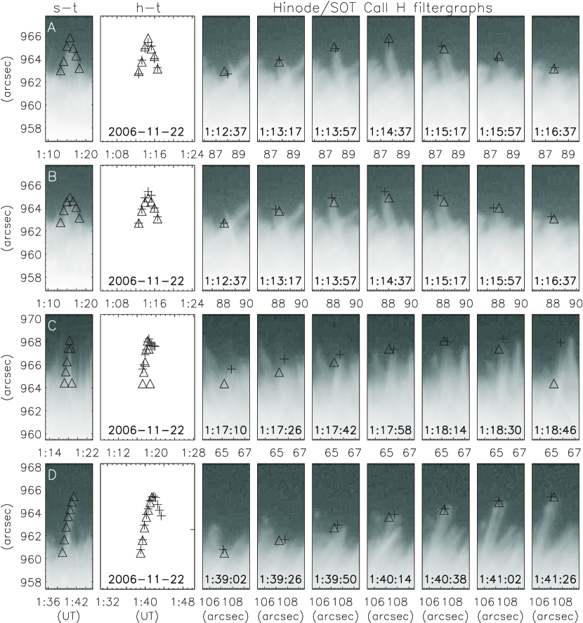
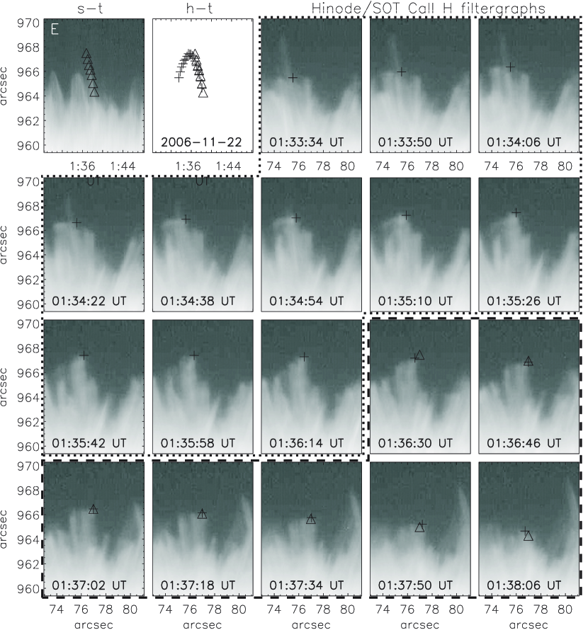
In the space-time diagrams, totally five typical morphology appearance of ‘spicules’ have been identified with large discrepancies of their lifetime and movement mode as classified by De Pontieu et al. (2007a). The ‘Type I’ spicules are indicated by ‘A’ and ‘B’ in Figure 1 and the ‘Type II’ spicules by ‘C’ and ‘D’ in Figure 1 and by ‘E’ in Figure 2. The tops denoted by triangles in Figure 1 and 2 are determined by the space-time plot at seven points of time for each case.

Yet, it is uncertain whether the ture height is obtained or not. To make sure of it, we try to find the tops of the ‘spicules’ in the filtergrams. In Figure 1, starting with the third panel, its seven panels in the row are the filtergrams corresponding to the seven points of time. The plus indicates the true height of the spicule directly determined by the filtergrams. The scatter plots in Figure 1 and 2 are used to compare the positions of the tops acquired by two methods, respectively. For example, in the panel marked with ‘A’ in Figure 1, the plus signs basically match those triangles. It means in this case the lifetime and height determined by space-time plot is basically true. However, in the case of ‘B’, the triangles are always slightly lower than those pluses though only several pixel distance apart between the slit for the space-time plot in the example ‘B’ and the one in the example ‘A’. The errors of the height measured in the way of space-time plot would produce errors in velocity and acceleration as well. In the sample ‘C’ we find that there are also great discrepancy in height measurement between two methods. In the space-time plot, the ‘spicule’ seems falling off suddenly, however, according to the filtergrams, the spicule falls more slowly and does not finish its whole life experience as shown in the corresponding scatter plots. The example ‘D’ is a more ‘typical’ ‘Type II’ spicule in space-time plot, but in the filtergram method the undetected descent phase by the first method did exist. As to the last example ‘E’ (shown in Figure 2) having a strange shape, the reason of lacking the ascent phase is that the first half process was not yet recorded in the space-time plot. The entire lifetime should include the panels enclosed by the dotted frame indicating the ascent phase and the dashed frame, the descent phase, but the space-time plot failed to detect the first part. Morphologically, in the space-time plots, as having been pointed out by De Pontieu et al. (2007a), two types of spicules are identified. But the approximately vertical stripes (‘Type II’ spicule) may be caused by the employment of the slit, which just cuts a part of the brightness distribution of a spicule, so that only a stripe of the distribution is left to be shown in the plots. For this reason, we hope to get statistical result of the spicule dynamic properties to answer if there are two types of spicules and their distributions in QS and CH.

2.3 The Measurement of the Kinetic Parameters of Spicule

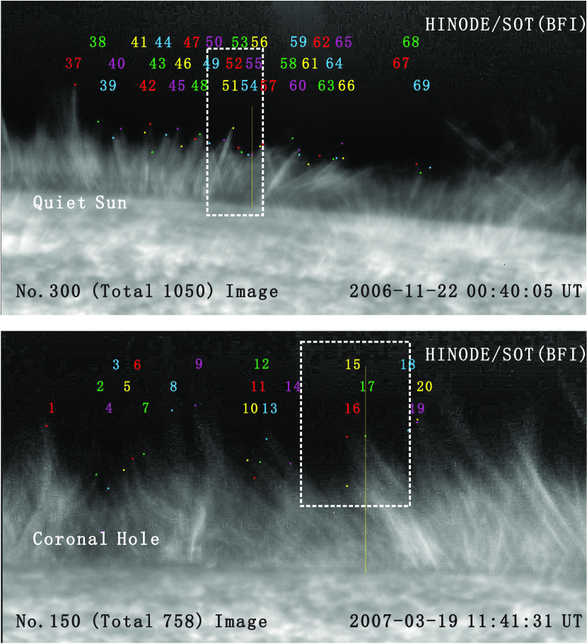
In the data set of QS, we identify 36, 33 and 36 spicules in three frames, i.e., Frames No. 100, 300 and 500 of total 1,050 filtergrams observed by Ca ii H filter, respectively. The upper panel of Figure 3 shows the No. 300 frame shot in QS at 00:40:05 UT on 2006 November 22. The tops of the identified 33 spicules (numbered 37 to 69) in this frame are marked by small squares in five color $\sbond$ red, green, blue, purple and yellow in turn, in the meanwhile their serial numbers are also written in the same color over the indicated spicules. The white dashed squares illustrate the FOVs of those filtergrams in Figures 4 and 5, respectively.

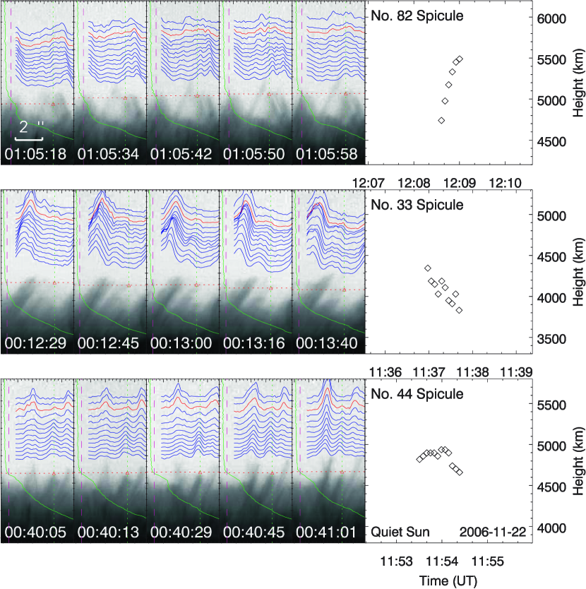
Figure 4 represents the time series of the dynamic process of No. 55 spicule in QS (hereafter called ‘SQ 55’). The spicule, as shown from the third panel to the third last panel, is detected from 00:39:57 UT to 00:43:17 UT. To find the top of the spicule at each time, based on the judgement with naked eyes, we used a set of brightness curves as an auxiliary measure to acquire more precise position for each top. These brightness curves reflect the brightness variation along the 13 horizontal lines with a two-pixel distance separating two adjacent lines. In case of these lines covering the spicule SQ 55, these brightness curves are plotted exactly above the spicule. Among them, the red brightness curve displays the brightness variation of the red dotted horizontal line. A spine shape is being gradually formed, becoming quite evident at about 00:41:09 UT, and then weakening slowly. At 00:43:17 UT, it was almost undetectable for its dropping to a lower position and then mixing with other spicules. The upper end of the spine, which is almost as weak as its ambient, should be the position of the top of the spicule at each moment. A series of red triangles corresponding to the time are used to indicate the spicule top positions. A green dotted vertical line and its concolorous brightness curve are plotted just as a reference. The brightness has an apparent variation around the top. A long red dashed vertical line marks the brightness value of 20 in vertical direction. In the bottom right panel in Figure 4, is the height-time plot, and the spicule height at each moment determined by the filtergrams is shown with the diamond. The apparent lifetime and height of the spicule SQ 55 are 200 seconds and 4,819 kilometers, respectively. The top trajectory marked by the diamonds shows a typical parabolic profile covering a complete cycle of acsent and descent. Before 00:39:57 UT and after 00:43:17 UT, due to the overlapping by a very large number of spicules, the SQ 55 could not be detected exactly. Evidently, the real lifetime should be longer than the apparent one, though we could not tell the real path of the spicule in which it was overlapped by other spicules. Totally, as shown by Table 1, there are 71 of 105 (67.6$\%$) spicules in QS moving upward firstly and then falling back. As for other 34 spicules, as shown in Figure 6, it seems that there are three different ‘types’ of spicules. The first ‘type’ only has the ascent phase, indicating by SQ 82; the second as SQ 33 just descending from higher to lower; and the last one, denoted by SQ 44, shows no obvious ascending and descending behaviors. Thus the profiles of these three types are likely the result of trajectory mixture with surrouding spicules. We still could not trace the whole life for individual.

In the data set of CH, similarly, from No. 150, 300, 450 and 600 frames, 20, 24, 34 and 24 spicules have been identified and traced , respectively. In the lower panel of Figure 3 is the No. 150 frame with 20 identified spicules indicated with the same symbols as above. The added white dashed frame is similar to the illustration of the FOV used in the filtergrams of Figure 5. Figure 5 shows the whole tracing process of No. 17 spicule in the coronal hole (hereafter called ‘SC 17’) from 11:40:43 UT to 11:44:38 UT, i.e. its apparent lifetime being 235 seconds. In contrast to the spicules in QS, the peaks of spicules in CH are too dim to be accurately detected. In the left lower panel of Figure 5, the tops at each time determined by frame tracing are shown in the height-time diagram. Apparently, SC 17 also experienced a complete cycle, up and then down. As listed by the right column of Table 1, total 102 spicules in CH, 64 (62.7$\%$), 24 (23.5$\%$), 6 (5.9$\%$) have been acquired the up- and downward, only upward, only downward phases; the remaining 8 (7.9$\%$) spicules without apparent upward or downward phase.

2.4 The Dynamic Properties of Spicules in QS and CH Regions

By tracing 105 and 102 spicule in QS and CH, we obtain the histograms of height, lifetime and vertical velocity shown in Figure 7. In panels A and B, the mean height in QS is 5,014 km ranged from 1,027 to 8,690 km, which is much lower than that, 9,592 km, from 4,819 to 17,142 km in CH. The average mean apparent lifetime in QS is 148 s, while in CH, it is 112 s, respectively. According to the height-time plot of each spicule in QS and in CH, we find that there are 71 of total 105 (about 67.6$\%$) spicules in QS and 64 of total 102 (about 62.7$\%$) in CH having a relatively complete cycle of ascent and descent. The reason of those spicules without a cycle basically lies in the disorder overlapping of a huge number of spicules. Hence for some spicules we observed the whole process of rising from the back of their adjacent spicules and then falling down; and for others only observed ascending, or descending or intermediate stage between. Therefore the measured lifetime should be shorter than their real lifetime. Yet, no one could tell what will occur when a spicule submerges in its background. Additionally, the velocity is basically proportional to the deceleration both in QS and in CH (see panels G and H in Figure 7).

3 Discussion and Conclusion

For the lateral motion of a spicule either in QS or in CH, no fixed slit could be employed in its whole lifetime. Therefore the spicule profile formed from space-time plot could not exactly represent the real trajectory of its movement. Comparing the kinematic parameters of spicules obtained in both methods, the height, lifetime acquired with the first method are always much less than those with the method we have adopted. That is why we do not use the space-time plot but employ its filtergrams directly to trace the trajectory of each spicule. Both in QS and in CH, are more than 60$\%$ spicules moving in a complete cycle of ascent and descent, and the rest showing no cycle suggested to be mixed in the background. In brief, with the same data sets in QS and in CH already used by De Pontieu et al. (2007a), no convincing ‘Type II’ spicule has been captured. Therefore, ‘Type I’, but not ‘Type II’ spicule dominates in QS and CH as shown in Table 1. This result is consistent with the study of spicules in the disk over QS (Suematsu, 1998) and over a plage (Anan et al., 2010) and at the limb (Pasachoff, 2009). It suggests that there is no a sufficient number of ‘Type II’ spicule to heat corona by their fading way both in QS and in CH.

Surely, there are apparent discrepancies in the dynamic properties of spicules in QS and in CH. The spicules in CH seem more energetic than those in QS (Shibata and Suematsu, 1982), for instance, they hit much higher position with higher speed and their lifetime is shorter. However, the relation between velocity and deceleration both in QS and in CH is approximately directly proportional associated with some different coefficient. There is a kind of faster spicules, but this does not mean that their physical mechanism is essentially different from that of other spicules.

With the help of the unprecedentedly high spatial resolution of Hinode/SOT Ca ii H filter, the identified diameter of spicule could be less than 200 km, which is much thinner than the values by observations in the past. However, it is still not easy to acquire a complete image of a limb spicule. Because of the faintness at the top of the spicule, there is some uncertainty in determining the top of a spicule (Rush and Roberts, 1954). At the lower position, as Lynch et al. (1973) pointed out, the spicules are so crowded, only when the visible spicules rise to some height and separate from each other far apart we could measure their kinetic parameters (Woltjer, 1954). It means that the measurement of the dynamic properties of spicules is far from being perfect. Thus the life story of these spicules remains somewhat vague. New instruments and technique are reasonably expected.

Last but not the least, when we watch the animation of Ca ii H filtergrams, spicules could form a ‘group’, moving in a similar way, such as dancing a waltz, or as a bamboo raft dispersing into individuals, etc. The ‘group’ motion may behave a more complicated behavior of a double thread structure of spicule having the following evolution (expansion thread separation, lateral motion and spinning as a whole body) (Suematsu, 2008; Sterling et al., 2010), which was speculated as magnetic reconnection. Thus, besides the energy taken by spicules themselves, these intensive activities will carry a huge amount of energy from chromosphere into corona. It may be the essentials of macrospicule and the practical way of releasing energy to corona. Our next work will pay more attention to measuring the kinematic parameters in 3D combining with ground-based Doppler observations in the line of sight (Shoji et al., 2010).

Table 1: The statistical dynamic properties of four ‘types’ of spicules

			QS					CH
Properties	Num.	H	LF	Vy	a	Num.	H	LF	Vy	a
		(km)	(s)	(km s-1)	(km s-2)		(km)	(s)	(km s-1)	(km s-2)
Up- and Downward	71	5174	176	16.9	-0.13	64	9572	121	48.0	-1.37
Only Upward	9	4792	74	11.2	-0.10	24	10,391	100	26.7	-0.22
Only Downward	11	4729	82	-9.6	0.05	6	8176	86	-6.7	-0.39
Uncertainty	14	4570	103	-	-	8	8418	95	-	-
Sum(Mean)	105	5014	148	15.5	-0.14	102	9592	112	40.5	-1.04

Notes–‘Num.’, ‘H’, ‘LF’, ‘Vy’, and ‘a’ means the number, mean height, mean lifetime, mean velocity in vertial direction and acceleration in vertial direction, respectively.

Figure 1: Comparison of two methods for tracking spicules. In the panels of the first column are four typical morphology appearance of ‘spicules’ determined by space-time plots; and the second column are the height-time plots. The last seven columns are Ca ii H filtergrams observed by Hinode/SOT. The triangle denotes the height acquired by space-time plot; as a comparison, the plus is the height obtained by frame tracking promptly.

Figure 2: Same as Figure 1 but for the fifth typical morphology appearance of ‘spicule’. The first panel in the top left shows the ‘spicule’ identified by the space-time plot; the second panel is then the height- time plots; from the third panel to the last one in the bottom right are the Ca ii H filtergrams observed by Hinode/SOT. The triangles and the pluses are the same as Figure 1.

Figure 3: Caii H images acquired by Hinode/SOT for quiet Sun at 00:40:05 UT on 2006 November 22 (upper panel) and coronal hole at 11:41:31 UT on 2007 March 19 (lower panel). Those colorful mini-squares marked the tops of identified spicules numbered with the concolorous Arabic numerals. The yellow lines denote the positions of slits to make space-time plots; white dashed frames are the field of view of filtergrams in Figure 4 and 5, respectively.

Figure 4: Time series of the dynamic processing of No. 55 SQ observed by Hinode/SOT Broadband Filter Imager in the Ca ii H on 2006 November 22. In each sub-images, red triangle marks the top of the spicule. The green solid curve is the brightness variation along the green dotted line. The red dashed line denotes the brightness value of 20. Similarly, the red solid curve is the brightness variation along the red dotted line. Two upper and ten lower cyan solid curves are also brightness variations along corresponding lines which are parallel to the red dotted line, but upper and lower than the red dotted line, respectively. The panel at the bottom right is the height-time plot of this spicule.

Figure 5: Time series of the dynamic process of No. 17 SC observed by Hinode/SOT Broadband Filter Imager in the Ca ii H on 2007 March 19. The lines have the same meaning as those described in Figure 4. The bottom right panel is the height-time plot of the spicule, too.

Figure 6: Time series of the dynamic process of other three ‘types’ of spicule and the related height-time plots. No. 82 is only observed at the ascent stage; No. 33 at the descent, but No. 44 spicule shows no obvious change in its height.

Figure 7: Histograms for QS (2006 November 22) and CH (2007 March 19). (A) and (B) the maximum height, (C) and (D) the lifetime, (E) and (F) the maximum vertical velocity. (G) and (H) are the scatter plot of spicule’s maximum velocity vs. its maximum deceleration in vertical direction.

References

- Anan et al. (2010) Anan, T. et al. 2010, PASJ, 62, 871
- Banerjee et al. (2000) Banerjee, D., O’Shea, E., Doyle, J. G. 2000, AA, 355, 1152
- Beckers (1972) Beckers, J. M. 1972, ARAA, 10, 73
- Bohlin et al. (1975) Bohlin, J. D., Vogel, S. N., Purcell, J. D., Jr. Sheeley, N. R., Tousey, R., Van Hoosier, M. E. 1975, ApJ, 197, L133
- Christopoulou et al. (2001) Christopoulou, E. B., Georgakilas, A. A., Koutchmy, R. G. 2001, Sol. Phys., 199, 61
- De Pontieu et al. (2007a) De Pontieu, B. et al. 2007a, PASJ, 59, 655
- De Pontieu et al. (2007b) De Pontieu, B. et al. 2007b, Science, 318, 1574
- Dere et al. (1989) Dere K. P., Bartoe, J. -D. F., Brueckner, G. E., Cook, J. W., Socker, D. G. 1989, Sol. Phys., 119, 55
- Hansteen et al. (2006) Hansteen, V. H., De Pontieu, B., Rouppe van der Voort, L., van Noort, M., and Carlsson, M. 2006, ApJ, 647, L73
- Hollweg et al. (1982) Hollweg, J. V., Jackson, S., Galloway 1982, Sol Phys., 75, 35
- Hollweg (1992) Hollweg, J. 1992, ApJ, 389, 731
- Ichimoto et al. (2005) Ichimoto, K. et al. 2005, in Proc. Chromospheric and Coronal Magnetic Fields, ESA SP-596, 81
- Ichimoto et al. (2008) Ichimoto, K. et al. 2008, Sol. Phys., 249, 233
- Ishikawa (2008) Ishikawa, R. et al. 2008, A&A, 481, 25
- Isobe et al. (2008) Isobe, H., Proctor, M. R. E., Weiss, N. O. 2008, ApJ, 679, L57
- Jin et al. (2009) Jin, C. L., Wang, J. X., Zhou, G. P. 2009, ApJ, 697, 693
- Kudoh and Shibata (1999) Kudoh, T., Shibata, K. 1999, ApJ, 514, 493
- Kulidzanishvili (1983) Kulidzanishvili, V. I. 1983, Sol. Phys., 88, 35
- Li and Ding (2009) Li, Y., Ding, M. D. 2009, RAA, 9, 829
- Lites et al. (2008) Lites, B. W. et al. 2008, ApJ, 672, 1237
- Lorrain and Koutchmy (1996) Lorrain, P., Koutchmy, S. 1996, Sol. Phys., 165, 115
- Lynch et al. (1973) Lynch, D. K., Beckers, J. M., Dunn, R. B. 1973, Sol Phys., 30, 63
- Matsumoto and Shibata (2010) Matsumoto, T., Shibata, K. 2010, ApJ, 710, 185
- Michard (1954) Michard, R. 1954, Obs, 74, 209
- Nikol’Skii and Sazanov (1967) Nikol’Sky, G. M., Sazanov, A. A. 1967, SvA, 10, 744
- Nishikawa (1988) Nishikawa, T. 1988, PASJ, 40, 613
- Okamoto et al. (2007) Okamoto, T. J. et al. 2007, Science, 318, 1577
- Pasachoff et al. (1968) Pasachoff, J. M., Noyes, R. W., Beckers, J. M. 1968, Sol Phys. 5, 131
- Pasachoff (2009) Pasachoff, J. M. et al. 2009, SP 260, 59
- Roberts (1945) Roberts, W. O. 1945, ApJ, 101-136
- Rouppe van der Voort et al. (2007) Rouppe van der Voort, L., De Pontieu, B., Hansteen, V. H., Carlsson, M., van Noort, M. 2007, ApJ, 660, L169
- Rush and Roberts (1954) Rush, J. H., Roberts, W. O. 1954, AuJPh, 7, 230
- Saito et al. (2001) Saito, T., Kudoh, T., Shibata, K. 2001, ApJ 554, 115
- Scharmer et al. (2003) Scharmer, G. B., et al. 2003, Proc. SPIE., 4853, 34
- Scullion et al. (2010) Scullion, E., Doyle, J. G., Erdlyi, R. 2010, Mem. S.A.It. 81, 737
- Secchi (1877) Secchi, P. A. 1877, Le Soleil,Vol. 2, Chap II. Paris: Gauthier-Villars
- Shibata and Suematsu (1982) Shibata, K., Suematsu, Y. 1982, Sol. Phys. 78, 333
- Shoji et al. (2010) Shoji, M., et al. 2010, PASJ 62, 927
- Sterling (2000) Sterling, A. C. 2000, Sol. Phys., 196, 79
- Sterling and Hollweg (1988) Sterling, A. C., Hollweg, J. V. 1988, ApJ, 327, 950
- Sterling et al. (2010) Sterling, A. C., Moore, R. L., DeForest, C. E. 2010, ApJ, 714, L1
- Suematsu et al. (1995) Suematsu, Y., Wang, H., Zirin, H. 1995, ApJ, 450, 411
- Suematsu (1998) Suematsu, Y. 1998, in solar jets and Coronal Plumes, ESA SP-421, 19
- Suematsu et al. (1982) Suematsu, Y., Shibata, K., Nishikawa, T., Kitai, R. 1982, Sol. Phys., 75, 99
- Suematsu (2008) Suematsu, Y. 2008, ASP conf. ser., 397, 27
- Suematsu et al. (2008) Suematsu, Y., et al. 2008, Sol. Phys., 249,197
- Suzuki and Inutsuka (2005) Suzuki, T. K., Inutsuka, S. 2005, ApJ, 632, L49
- Suzuki and Inutsuka (2006) Suzuki, T. K., Inutsuka, S. 2006, J. Geophys. Res., 111, A06101
- Takeuchi and Shibata (2001) Takeuchi, A., Shibata, K. 2001, ApJ, 546, L73
- Tavabi et al. (2011) Tavabi, E., Koutchmy, S., Ajabshirizadeh, A. 2011, AdSpR, 47, 2019
- Thomas and Athay (1961) Thomas, R. N., and Athay, R. G. 1961, Physics of the Solar Chromosphere (New York: Interscience)
- Tsuneta et al. (2008) Tsuneta, et al. 2008, Sol. Phys., 249, 167
- Weart (1970) Weart, S. R. 1970, Sol. Phys. 14,310
- Wilhelm (2000) Wilhelm, K. 2000, AA, 360, 351
- Woltjer (1954) Woltjer, L. 1954, BAN, 12, 165
- Xia et al. (2005) Xia, L. D., Popescu, M. D., Doyle, J. G., Giannikakis, J. 2005, AA, 438, 1115
- Zaqarashvili and Erd´elyi (2009) Zaqarashvili, T. V., Erdlyi, R. 2009, SSRv, 149, 355
- Zhang et al. (2009) Zhang, J., Yang, S. H., Jin, C. L. 2009, RAA 9, 921