Computing Nash Equilibrium in Wireless Ad Hoc Networks: A Simulation-Based Approach

Abstract

This paper studies the problem of computing Nash equilibrium in wireless networks modeled by Weighted Timed Automata. Such formalism comes together with a logic that can be used to describe complex features such as timed energy constraints. Our contribution is a method for solving this problem using Statistical Model Checking. The method has been implemented in Uppaal model checker and has been applied to the analysis of Aloha CSMA/CD and IEEE 802.15.4 CSMA/CA protocols.

1 Introduction

One of the important aspects in designing wireless ad-hoc networks is to make sure that a network is robust to the selfish behavior of its participants. This problem can be formulated in terms of a game considering that network nodes behave in a rational way and want to maximize their utility. A wireless network is robust iff its configuration satisfies Nash equilibrium (NE), i.e. it is not profitable for a node to alter its behavior to the detriment of other nodes.

In this paper we propose a new methodology to compute NE in wireless ad-hoc networks. Our approach is based on Statistical Model Checking (SMC) [25, 19], an approach used in the formal verification area. SMC has a wide range of applications in the areas such as systems biology or automotive. The core idea of SMC is to monitor a number of simulations of a system and then use the results of statistics (e.g. sequential analysis) to get an overall estimate of the probability that the system will behave in some manner. Thus SMC can help to overcome the undecidability issues, that arise in the formal analysis of wireless ad-hoc networks [2]. While the idea ressembles the one of classical Monte Carlo simulation, it is based on a formal semantics of systems that allows us to reason on very complex behavioral properties of systems (hence the terminology). This includes classical reachability property such as “can i reach such a state?”, but also non trivial properties such as “can i reach this state x times in less than y units of time?”.

Here we use a semantics for systems that is based on timed automata. We assume that elements of a network are modeled using Weighted Timed Automata (WTA), that is a model for timed system together with a stochastic semantics. The model permits, for example, to describe stochastically how the behaviors of a system involve with respect to time. As an example, probability can be used to say that the system is more likely to move to the next state in five units of time rather than in ten. Our approach permits to describe arbitrary distributions when combining individual components. In addition, WTA are equiped with nice communication primitives between components, including e.g. message passing. The fact that we rely on WTA allows us to describe utility functions with cost constraint temporal logic called PWCTL. PWCTL is a logic that allows to temporally quantify on behaviors of components as well as on their individual features (cost, energy consumption). By the existing results, we know that one can always define a probability measure on sets of run of a WTA that satisfy a given property written in cost constraint temporal logic. The latter clearly arises the importance of defining a formal semantics for system’s models.

Going back to modeling wireless ad-hoc network, we will assume that each node can work according to one out of finitely many configurations that we call strategies (a strategy being a choice of a configuraiton). We also assume that each network node has a goal and a node’s utility function is equal to the probability that this goal will be reached on a random system run. Each node will be represented with a WTA and a goal will be described with PWCTL. Our algorithm for computing NE consists of two phases. First, we apply simulation-based algorithm to compute a strategy that most likely (heuristic) satisfies NE. This is done by monitoring several runs of the systems with respect to a property and then use classical Monte Carlo ratio to estimate the probability that this strategy is indeed the good one. In the second phase we apply statistics to test the hypothesis that this strategy actually satisfies NE. Indeed, it is well-known that such a NE may not exist [17], so our statistical algorithm goes for the best estimate out of it that corresponds to a relaxed NE for the system.

We implemented a distributed version of this algorithm that uses Uppaal statistical model checker as a simulation engine [14]. The Uppaal toolset offers a nice user interface that makes it one of the most widely used formal verification based tool in academia. Thanks to the independent simulations that the algorithm generates, this problem can easily be parallelized and distributed on, e.g., PC clusters.

Finally, we apply our tool to the analysis of two probabilistic CSMA (Carrier Sense Multiple Access) protocols: k-persistent Aloha CSMA/CD protocol and IEEE 802.15.4 CSMA/CA protocol. The two case studies we present in this paper serve mainly demonstration purposes. However, we are the first who study Nash Equilibrium in unslotted Aloha (the slotted version of Aloha was previously studied in [20] and [24]). Our result that there exists only “always transmit” Nash Equilibrium strategy in IEEE 802.15.4 CSMA/CA reproduces the analogous result for the IEEE 802.11 CSMA/CA protocol [10].

The problem of computing Nash Equilibrium in wireless ad-hoc networks was first considered in [20] and surveid in [24]. Most of existing works are based on an analytical solution which does not scale well with complex models [16, 20]. Similarly to us, some other works [10] are based on a simulation-based approach. However, contrary to us, they do not assign any statistical confidence to the results, and they do not take advantage of temporal logic to express arbitrary objectives.

2 Weighted Timed Automata

In this section, we briefly recap the concept of Weighted Timed Automata (WTA), see [13] for more details. We denote ${\cal{B}}(X)$ to be a finite conjunction of bounds of the form $x\sim n$ where $x\in X$, $n\in\bbbn$, and $\sim\in\{<,\leq,>,\geq\}$.

Definition 1

A Weighted Timed Automaton (WTA) is a tuple ${\cal A}=(L,\ell_{0},X,E,R,I)$ where: (i) $L$ is a finite set of locations, (ii) $\ell_{0}\in L$ is the initial location, (iii) $X$ is a finite set of real-valued variables called clocks, (iv) $E\subseteq L\times{\cal{B}}(X)\times 2^{X}\times L$ is a finite set of edges, $(v)$ $R:L\rightarrow\mathbb{Z}_{\geq 0}$ assigns a rate vector to each location, and (vi) $I:L\rightarrow{\cal{B}}(X)$ assigns an invariant to each location.

A state of a WTA is a pair $(l,v)$ that consists of a location $l$ and a valuation of clocks $\nu:X\rightarrow\bbbr_{\geq 0}$. From a state $(l,v)\in L\times\bbbr_{\geq 0}^{X}$ a WTA can either let time progress or do a discrete transition and reach a new location. During time delay clocks are growing with the rates defined by $R(l)$, and the resulting clock valuation should satisfy invariant $I(l)$. A discrete transition from $(l,v)$ to $(l^{\prime},v^{\prime})$ is possible if there is $(l,g,Y,l^{\prime})\in E$ such that $v$ satisfies $g$ and $v^{\prime}$ is obtained from $v$ by resetting clocks from the set $Y$ to $0$. A run of WTA is a sequence of alternating time and discrete transitions. Several WTA $M_{1},M_{2},\dots,M_{n}$, can communicate via inputs and outputs to generate Networks of WTAs (NWTAs) $M_{1}\|M_{2}\|\dots\|M_{n}$.

In our early works [13], the stochastic semantics of WTA components associates probability distributions on both the delays one can spend in a given state as well as on the transition between states. In Uppaal uniform distributions are applied for bounded delays and exponential distributions for the case where a component can remain indefinitely in a state. In a network of WTAs the components repeatedly race against each other, i.e. they independently and stochastically decide on their own how much to delay before outputting, with the “winner” being the component that chooses the minimum delay. As observed in [13], the stochastic semantics of each WTA is rather simple (but quite realistic), arbitrarily complex stochastic behavior can be obtained by their composition when mixing individual distributions through message passing. The beauty of our model is that these distributions are naturally and automatically defined by the network of WTAs.

Our implementation supports extension of WTA, coming from the language of the Uppaal model checker [18]. Such models can contain integer variables that can be present in transition guards, and they can be updated only when a discrete transition is taken. Additionally, we support other features of the Uppaal model checker’s input language such as data structures and user-defined functions.

A parametrized WTA $M(p)$ is a WTA in which some integer constant (transition weight or constant in variable assignment/clock invariant) is replaced by a parameter $p$.

For defining properties we use cost-constraint temporal logic PWCTL, which contains formulas of the form $\Diamond_{c\leq C}\phi$. Here $c$ is an observer clock (that is never reset and grows to infinity on any infinite run of a WTA), $C\in\bbbr_{\geq 0}$ is a constant and $\phi$ is a state-predicate. We say that a run $\pi$ satisfies $\Diamond_{c\leq C}\phi$ if there exists a state $(l,v)\in\pi$ in this run such that it satisfies $\phi$ and $v(c)\leq C$. We define $Pr[M\models\psi]$ to be equal to the probability that a random run of $M$ satisfies $\psi$.

3 Modeling Formalism and problem statement

We consider that each node operates according to one out of finitely many configurations. Thus a network of $N$ nodes can be modelled by:

$$S(p_{1},p_{2},\dots,p_{N})\equiv M(p_{1})\|M(p_{2})\|\dots\|M(p_{N})\|C$$ (1)

where $M$ is a parametrized model of a node, $p_{i}\in P$ (i.e, the behavior of a node relies on some value - strategy - assigned to the parameters), $P$ is a finite set of configurations and $C$ is a model of a medium.

Consider a parameterized NWTA $S(p_{1},p_{2},\dots,p_{N})$ that models a wireless network of $N$ nodes. Here each $p_{i}$ defines a configuration of a node $i$ and ranges over a finite domain $P$. Since the players (nodes) are symmetric, we can analyze the game from the point of view of the first node only. Thus we will consider the goal of the first node only, and this goal is defined by a PWCTL formula $\psi$.

We can view a system as a game $G=(N,P,U)$, where $N$ is a number of players (nodes), $P$ is a set of strategies (parameters) and $U:P^{N}\rightarrow[0,1]$ is an utility function of the first player defined as

$$U(p_{1},p_{2},\dots,p_{N})\equiv Pr[S(p_{1},p_{2},\dots,p_{N})\models\psi]$$ (2)

We consider that there is a master node that knows the network configuration (here the number of nodes) and broadcasts the strategy (parameter) that all the nodes should use.

If all the nodes are honest, they will play according to the strategy proposed by the master node. Thus in this case the master node should use a symmetric optimal strategy, i.e. a strategy $p$ such that for all other strategies $p^{\prime}$ we have $U(p,p,\dots,p)\geq U(p^{\prime},p^{\prime},\dots,p^{\prime})$.

However, if there are selfish nodes, they might deviate from the symmetric optimal strategy to increase the value of their utility functions (and the rest of the nodes can possibly suffer from that). Thus we will consider a Nash Equilibrium strategy that is stable with respect to the behavior of such selfish nodes (but possibly this strategy is less efficient than the symmetric optimal one). More formally, a strategy $p$ is said to be a Nash Equilibrium (NE), iff for all $p^{\prime}\in P$ we have $U(p,p,\dots,p)\geq U(p^{\prime},p,\dots,p)$.

However, a Nash Equilibrium may not exist [17], thus in this paper we will consider a relaxed definition of Nash Equilibrium.

Definition 2

A strategy $p$ satisfies symmetric $\delta$-relaxed NE iff for all $p^{\prime}\in P$ we have $U(p,p,\dots,p)\geq\delta\cdot U(p^{\prime},p,\dots,p)$.

The value of $\delta$ measures the quality of a strategy $p$. If $\delta\geq 1$, then $\delta$-relaxed NE satisfies the traditional definition of the (non-relaxed) NE. Otherwise, if $1-\delta$ is small, then we can conclude that a node’s gain of switching is negligible and it’ll stick with the $\delta$-relaxed NE strategy. A $\delta$-relaxed NE strategy can be also used when a set of possible strategies is infinite. In this case we can discritize this set (approximate it by a finite set of strategies) and search for a $\delta$-relaxed NE strategy in this finite set. If an utility function is smooth, then this strategy can be a good approximation for a NE in the original (infinite) set of strategies.

In this paper, we will solve the problem of searching for a strategy that satisfies $\delta$-relaxed NE for as large $\delta$ as it is possible.

For readability, in the rest of the paper we will write $U(p^{\prime},p)$ and $S(p^{\prime},p)$ instead of $U(p^{\prime},p,\dots,p)$ and $S(p^{\prime},p,\dots,p)$, respectively.

4 Algorithm for Computing Nash Equilibrium

One may suggest that in order to compute NE we can compute the values of $U(p^{\prime},p)$ for all pairs $(p^{\prime},p)$ and then use definition 2 to compute the maximal value of $\delta$. However, we can’t do that because the problem of evaluating PWCTL formula on a model (i.e. computing $Pr[S\models\psi]$) is undecidable in general for WTA [8].

In this paper, we will use Statistical Model Checking (SMC) [19] based approach to overcome this undecidability problem. The main idea of this approach is to perform a large number of simulations and then apply the results of statistics to estimate the probability that a system satisfies a given property.

Our method of computing NE consists of two phases. During the first phase (presented in Section 4.1) we apply a simulation-based algorithm to search for the best candidate $p$ for a Nash Equilibrium. Then, in the second phase (presented in Section 4.2), we apply statistics to evaluate $p$, i.e. to find the maximum $\delta$ such that with a given significance level we can accept the statistical hypothesis that $p$ is a $\delta$-relaxed Nash Equilibrium.

In the rest of the paper, we use straightforward simulation-based Monte Carlo method for computing estimations of utility function’s values. In this method we perform $n$ random simulations of $S(p^{\prime},p)$ for a given pair $(p^{\prime},p)$ and count the number $k$ of how many simulations satisfied $\psi$. Then we use the following estimation: $\widetilde{U}(p^{\prime},p)=k/n$.

4.1 Finding a Candidate for a Nash Equilibrium

Algorithm 1 Computation Of The Best Candidate For Nash Equilibrium

Input: $P=\{p_{i}\}$ — finite set of parameters, $U(p_{i},p_{k})$ — utility function, $d\in[0,1]$ — threshold
Algorithm:
1. for every $p_{i}\in P$ compute estimation $\widetilde{U}(p_{i},p_{i})$
2. $waiting$ := $P$
3. $candidates$ := $\emptyset$
4. while $len(waiting)>1$:
5. pick some unexplored pair $(p_{i},p_{k})\in P\times waiting$
6. compute estimation $\widetilde{U}(p_{i},p_{k})$
7. if $\widetilde{U}(p_{k},p_{k})<d\cdot\widetilde{U}(p_{i},p_{k})$:
8. remove $p_{k}$ from $waiting$
9. else if $\forall p_{i}^{\prime}$ $\widetilde{U}(p_{i}^{\prime},p_{k})$ is already computed
10. remove $p_{k}$ from $waiting$
11. add $p_{k}$ to $candidates$
12. return $\mathop{argmax}_{p\in candidates}\min_{p^{\prime}\in P}(\widetilde{U}(p,p)/\widetilde{U}(p^{\prime},p))$

As a first step, the algorithm computes estimations $\widetilde{U}(p^{\prime},p)$ for various $p^{\prime}$ and $p$ and search for a parameter $p$ that maximizes the value of $\min_{p^{\prime}\in P}(\widetilde{U}(p,p)/\widetilde{U}(p^{\prime},p))$.

Additionally, we speedup the search by introducing a heuristic threshold $d$ (that is a parameter of our algorithm) and pruning parameters $p$ such that $\widetilde{U}(p,p)/\widetilde{U}(p^{\prime},p)<d$.

Our algorithm (see Algorithm 1) starts with the computation of estimations $\widetilde{U}(p_{i},p_{k})$ at diagonal points (i.e. when $i=k$). After that we iteratively pick a random pair of strategies $(p_{i},p_{k})$ and compute $\widetilde{U}(p_{i},p_{k})$. If $\widetilde{U}(p_{k},p_{k})/\widetilde{U}(p_{i},p_{k})<d$, then we remove strategy $p_{k}$ from the further consideration and will never consider again pairs of the form $(?,p_{k})$.

We iterate the while-loop until we split all the parameters into those $p$ for which we already computed the value of $\min_{p^{\prime}\in P}(\widetilde{U}(p,p)/\widetilde{U}(p^{\prime},p))$, and those, for which we know that $\widetilde{U}(p,p)/\widetilde{U}(p^{\prime},p)<d$ for some $p^{\prime}$. Then at line 12 we choose a strategy $p$ that maximizes $\min_{p^{\prime}\in P}(\widetilde{U}(p,p)/\widetilde{U}(p^{\prime},p))$

It should be noted, that if a threshold $d$ is large, then our algorithm can possibly return no result (because all the candidates will be filtered out). In this case one can retry with a smaller $d$ and reuse the already computed estimations. If $d$ is equal to zero, then the algorithm is guaranteed to return a result.

4.2 Evaluation of a Relevance of the Candidate

Consider that after the first phase we selected a strategy $p$. Let $H_{p,\delta}$ be a statistical hypothesis that $p$ is a $\delta$-relaxed NE. Now we want to find the maximal $\delta$ such that we can accept the hypothesis $H_{p,\delta}$ with a given significance level $\alpha$ (that is a parameter of the algorithm).

To do that we firstly reestimate $\widetilde{U}(p^{\prime},p)$ for every $p^{\prime}\in P$ (possibly using the number of simulations that is different from the one that was used in the first phase, this will be discussed below).

Then we apply the following theorem:

Theorem 1

Suppose that for all $p^{\prime}\in S$ we estimated $\widetilde{U}(p^{\prime},p)$ using $n$ random simulations, and $f(\delta)\leq\alpha$, where

$$f(\delta)\equiv\sum_{i=1..N}\frac{1}{2}\Big{(}1-\mathop{erf}\big{(}\sqrt{n}({\widetilde{U}(p,p)-\delta\cdot\widetilde{U}(p_{i},p)})\big{)}\Big{)}$$ (3)

and $\mathop{erf}(x)=\frac{2}{\sqrt{\pi}}\int_{0}^{x}e^{-t^{2}}dt$ is Gauss error function. Then we can accept the statistical hypothesis $H_{p,\delta}$ with the significance level of $\alpha$.

Proof 4.2.

Let ${q}_{i}={U}(p_{i},p_{k})$ and $\widetilde{q}_{i}=\widetilde{U}(p_{i},p_{k})$. Then $p_{k}$ satisfies $\delta$-relaxed Nash Equilibrium iff $\forall i\cdot q_{k}\geq\delta q_{i}$ Consider that we have $n$ Bernoulli random variables $\zeta_{1},\zeta_{2},\dots,\zeta_{n}$ where $Pr[\zeta_{i}=1]=q_{i}$. Consider that random variable $\xi_{i}$ is a mean of $n$ independent observations of $\zeta_{i}$, i.e. $\xi_{i}=\sum_{j=1..n}\zeta_{i}/n$ Then each $\widetilde{q}_{i}$ is an independent observation of $\xi_{i}$ and for large $n$ we have $\xi_{i}\sim\mathcal{N}(q_{i},q_{i}(1-q_{i})/n)$. Probability of making type II error (accept $H_{p_{k},\delta}$ when it is false) is less or equal to

$$Pr[\xi_{1}=\widetilde{q}_{1},\xi_{2}=\widetilde{q}_{2},\dots,\xi_{n}=\widetilde{q}_{N}\|\bigvee_{i=1..N}q_{k}<\delta\cdot q_{i}]$$ (4)

, that in turn is less or equal to

$$\sum_{i=1..N}Pr[\xi_{1}=\widetilde{q}_{1},\xi_{2}=\widetilde{q}_{2},\dots,\xi_{n}=\widetilde{q}_{N}\|q_{k}<\delta\cdot q_{i}]$$ (5)

, that in turn is less or equal to

$$\sum_{i=1..N}Pr[\xi_{i}=\widetilde{q}_{i},\xi_{k}=\widetilde{p}_{k}\|q_{k}<\delta\cdot q_{i}]$$ (6)

, that in turn is less or equal to

$$\sum_{i=1..N}Pr[(\xi_{k}-\delta\cdot\xi_{i})=(\widetilde{q}_{k}-\delta\cdot\widetilde{q}_{i})\|q_{k}-\delta\cdot q_{i}<0]$$ (7)

For each $i$ we have:

$$(\xi_{k}-\delta\cdot\xi_{i})\sim\mathcal{N}(q_{k}-\delta q_{i},(q_{k}(1-q_{k})+q_{i}(1-q_{i}))/n)$$ (8)

The truth of the theorem follows from the fact that $q_{k}(1-q_{k})+q_{i}(1-q_{i})\leq 0.5$. ∎

We apply this theorem in the following way. We first search for an integer-valued $b$ such that $f(b)<0$. Then we use bisection numerical method to find a root of an equation $f(\delta)=\alpha$ on the interval $[0,b]$. It can be easily seen that the function $f$ decreases and $f(0)>0$ and it implies that this $\delta$ satisfies the condition of the theorem.

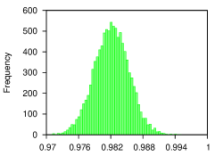
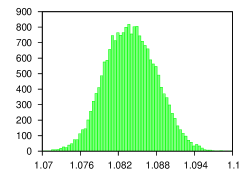
Figure 1: The experimental evaluation of the application of theorem 1. In the upper plots the $x$ axis denotes the number of simulations $n$, and $y$ axis denotes an average estimated value of $\delta$ computed using theorem 1 for these numbers of simulations and the significance level of $\alpha=0.05$. $N$ is the total number of strategies. The bottom plots demonstrate the frequency distribution for the computed values of $\delta$ for $100000$ simulations and $100$ possible strategies. The left and right plots correspond to the cases when the real value of $\delta$ is equal to $1.0$ and $1.1$.

Our method provides only a lower bound for $\delta$ and the theorem 1 does not state how many simulations are needed to compute a good estimation of $\delta$. Indeed, we can compute statistically valid $\delta$ for any number of simulations. And if the estimated value of $\delta$ is small, it can be a result of the fact that the number of simulations is insufficient or the real value of $\delta$ is small (or both).

Thus we performed an experiment to see how accurate is our method depending on the number of simulations. We developed a simple model of our method, and in this model we assume that there are $N$ strategies $\{p_{1},p_{2},\dots p_{N}\}$, and we want to check that $p_{1}$ is a Nash Equilibrium. The value of the utility function $U(p_{1},p)$ is equal to $0.5$ for $p\neq p_{1}$, and it is equal to $0.5\cdot\delta$ when $p=p_{1}$ (thus $p_{1}$ is a $\delta$-relaxed NE). The experimental data for the cases when $\delta=1.0$ and $\delta=1.1$ is presented at Fig. 1. A reader can see that the results for these two cases are similar, and our other experiments (with $\delta$ ranging from $0.5$ to $2.0$) also demonstrate this similarity. The accuracy of our method increases as the number of simulation $n$ increases or the number of possible strategies $N$ decreases. One can also see, that for this experiment $100000$ simulations seem to be enough to compute a good approximation for $\delta$ that is both statistically valid (this is ensured by the theorem 1) and close to the real value of $\delta$.

4.3 Implementation Details

We developed a tool written in Python programming language that implements the proposed algorithm. This tool uses Uppaal model checker as a simulation and monitoring engine for PWCTL properties.

Our algorithm is based on Monte Carlo simulations and thus it is embarrassingly parallisable. In our implementation we exploit this parallelisability by computing the estimations for different pairs of strategies on different nodes. The tool can be run on a cluster. One node acts as a master and picks the parameters $p_{i}$, $p_{j}$ that the slave nodes use to compute the estimations $\widetilde{U}(p_{i},p_{j})$. The master node does not use any external job scheduler and submits jobs on its own using SSH connection to the computational nodes. Currently we rely on the fact that the nodes share the same distributed file system, but in principle the master node can deploy all executables and models by itself.

5 Results of Application

In this paper we report on results of application of our tool to two contention resolution protocols. The first one is Aloha CSMA/CD protocol that we model on a very abstract level and we’ll describe our model in details. The second one is IEEE 802.15.4 CSMA/CA that we model with a high precision and we’ll just briefly sketch its structure.

For both case studies we used the following parameters. The number of simulations for estimation of utility function’s values is equal to $10000$ for the first phase of our algorithm (searching for the best candidate for NE) and $100000$ for the second phase (evaluation of this candidate). The value of $d$ parameter is equal to $0.9$, and the value of significance level $\alpha$ is equal to $0.05$.

All the experiments were performed on the $8$ node cluster, where each node has an Intel^© Core^®2 Quad CPU.

5.1 Application to Aloha CSMA/CD protocol

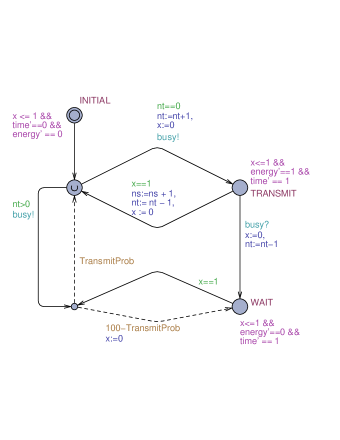
Figure 2: Model of Aloha in Uppaal

Aloha protocol [3] is a simple Carrier Sense Multiple Access with Collision Detection (CSMA/CD) protocol that was used in the first known wireless data network developed at the University of Hawaii in 1971.

In this protocol it is assumed that there are several nodes that share the same wireless medium. Each node is listening to its own signal during its transmission and checks that the signal is not corrupted by another node’s transmission. In case of collision both nodes will stop transmitting immediately and wait for a random time before they’ll try to transmit again.

In our paper we consider unslotted Aloha in which the nodes are not necessary synchronized. Additionally, we study k-persistent variant of Aloha, i.e. a protocol implementation in which a random delay before retransmission is distributed according to a geometric distribution. This means that for each next time slot a node will transmit with probability TransmitProb and will wait for one more slot (and then decide again) with probability $1-$TransmitProb. We assume that a node can change the value of TransmitProb, thus a strategy of a node consists of choosing a value of TransmitProb. We also assume that a node can use one out of $100$ of discretized values $\{0.01,0.02,\dots,1\}$ of TransmitProb.

The Uppaal model of a single node is presented at Fig. 2. Wireless media is modeled using a broadcast channel busy (in which a signal is sent each time a new transmission starts) and integer variable nt (that stores the number of stations that are currently transmitting). Variable ns stores the number of successful transmissions. Time can pass only in locations INITIAL, TRANSMIT and WAIT, two other locations are urgent. A node uses clocks x, time (that stores a time passed since the beginning) and energy (that stores the amount of energy consumed, i.e. the amount of time spent in the location TRANSMIT).

We assume that there is a random uniformly distributed offset between the initial states of the nodes (it is modeled by delay in location INITIAL). This may correspond to the situation, when there is a wireless sensor network and all sensors are aimed towards the same event. As soon as this event happens, all the node will start transmission, but they will not be necessarily synchronized.

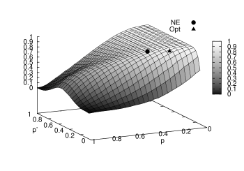
Figure 3: $\widetilde{U}(p^{\prime},p)$ (left) and its diagonal slice (right) for Aloha with $5$ nodes

Number of nodes	2	3	4	5	6	7	8
$\delta$-relaxed NE strategy $p_{NE}$	0.37	0.40	0.35	0.35	0.41	0.42	0.41
Value of $\delta$	0.992	0.980	0.992	0.990	0.993	0.992	0.987
$\widetilde{U}(p_{NE},p_{NE})$	0.99	0.98	0.95	0.89	0.75	0.61	0.50
Symmetric optimal strategy $p_{opt}$	0.30	0.30	0.26	0.22	0.19	0.15	0.14
$\widetilde{U}(p_{Opt},p_{opt})$	0.99	0.98	0.96	0.90	0.87	0.98	0.76
Computation time	2m5s	3m44s	7m62s	15m45s	26m11s	37m55s	59m15s

Table 1: Nash equilibrium (NE) and Symmetric optimal (Opt) strategies for Aloha

In our experiments we assumed that the goal of a node is to transmit a single frame within $50$ time units and to limit energy consumption by $3$. This goal can be expressed using the following PWCTL formula:

$$\Diamond_{\mbox{{\tt Node(0).time}}\leq\mbox{{\tt 50}}}(\mbox{{\tt Node(0).ns}}\geq\mbox{{\tt 1}}\wedge\mbox{{\tt Node(0).energy}}\leq\mbox{{\tt 3}})$$ (9)

It should be noted, that even our (unslotted) Aloha model looks simple, we can’t propose an analytical way of computing $U(p^{\prime},p)$ for a given values of $p^{\prime}$ and $p$. The problem is that our model works in real-time and we can’t decompose its behavior into rounds (slots) and compute $U(p^{\prime},p)$ recursively based on the nodes’ actions in the current round and values of $U(p^{\prime},p)$ in the next possible rounds (like it was done in [20] for slotted Aloha).

Fig. 3 depicts the plot of the utility function estimation $\widetilde{U}(p^{\prime},p)$ for the first player for the network of $5$ nodes (remind, that $p^{\prime}$ is a strategy of the first player, and $p$ is common strategy of all the other players). It also shows Nash Equilibrium (NE) and symmetric optimal (Opt) strategies. It should be noted, that due to the usage of $d$ parameter our algorithm didn’t compute $\widetilde{U}(p^{\prime},p)$ for all possible $p$ and $p^{\prime}$ (in fact, only $3742$ out of $10000$ values were computed).

Intuitively, a Nash Equilibrium for Aloha exists, because a node has to satisfy both time and energy constraints. When the honest nodes use the value of TransmitProb that is close to $1$, it forces the selfish node to use a smaller value of TransmitProb to bound the number of collisions (and hence the energy consumption). When the default value of TransmitProb is close to $0$, the selfish node uses a larger value of TransmitProb to decrease the expected time before the next retransmission, since the probability of a collision is small for this case. This ensures that a Nash Equilibrium strategy exists in between $0$ and $1$.

Table 1 contains the results for ALOHA with different number of nodes. It can be seen, that relaxed NE and symmetric optimal strategies coincide for the case of two network nodes, but for the networks with more nodes relaxed NE is less efficient than symmetrical optimal strategy.

5.2 Application to IEEE 802.15.4 CSMA/CA Protocol

IEEE 802.15.4 standard [23] specifies the physical layer and media access control layer for low-cost and low-rate wireless personal area networks. Upper layers are not covered by IEEE 802.15.4 and are left to be extended in industry and individual applications. One of such extensions is ZigBee [4] that together with IEEE 802.15.4 completes description of a network stack. Typical applications of ZigBee include smart home control and wireless sensor networks.

We applied our tool to the analysis of Multiple Access/Collision Avoidance (CSMA/CA) network contention protocol being a part of IEEE 802.15.4. Unlike Aloha, the IEEE 802.15.4 standard assumes that a wireless node can’t listen to its own transmission and thus it is not possible to detect a collision as soon as it occurs and stop transmission. A node will detect a collision later when it does not receive an acknowledgment within a given time bound. Before each transmission a node performs a Clear Channel Assessment (CCA), i.e. checks that no other node is transmitting. If CCA was not successful (the medium was busy), then the node waits for a random time before performing CCA again, and this time is distributed according to the binary exponential backoff mechanism (that is controlled by the parameters MinBE, MaxBE and UnitBackoff in our model). If CCA was successful (the medium was clear), then the node switches to the transmitting mode and starts transmission. However, this switching takes non-zero time (TurnAround in our model), and another node can start transmitting during this period, that will lead to a collision.

The standard defines both slotted (with beacon synchronization) and unslotted modes of CSMA/CA; in our paper we consider only unslotted one.

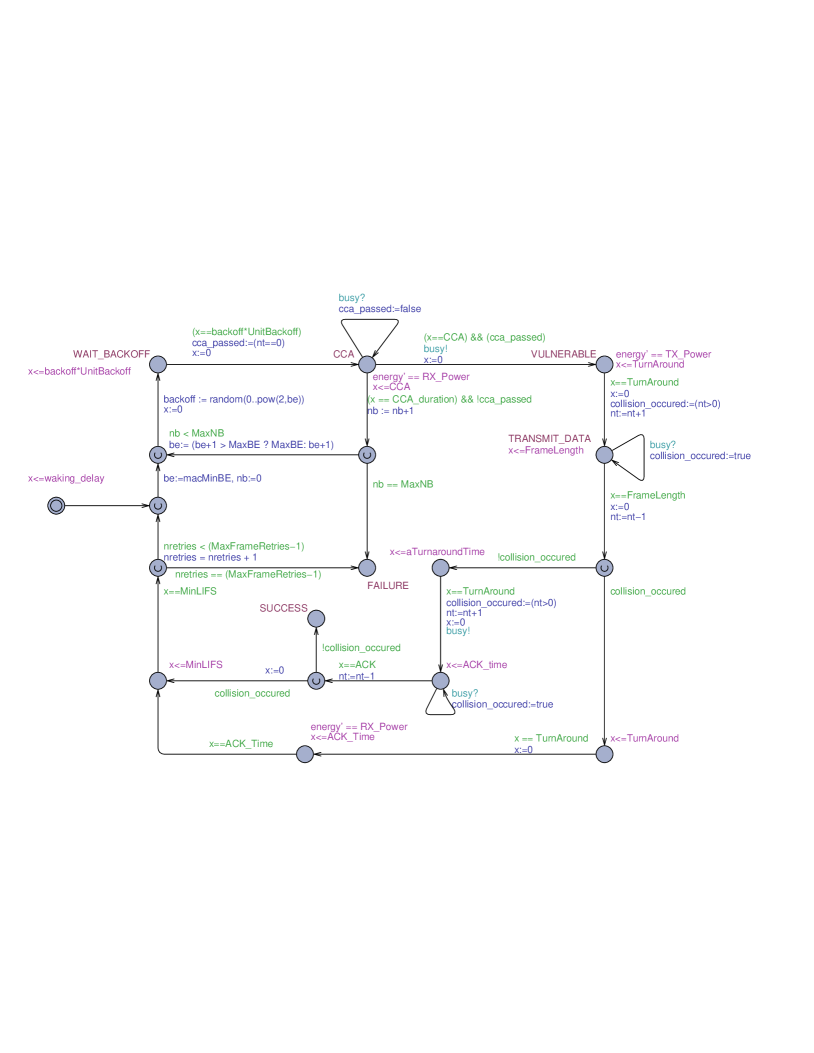
Figure 4: Model of IEEE 802.15.4 CSMA/CA

The model of a single node operating according to IEEE 802.15.4 CSMA/CA is depicted at Fig. 4. The values of MinBE, MaxBE, MaxFrameRetries, TurnAround were taken from the IEEE 802.15.4 standard assuming that the network is operating on baud rate 20kbps and on 868 Mhz band. FrameLength is considered to be 35 bytes (including 25 bytes for ZigBee header and 10 bytes for the valuable information). We assume that the frame size is 35 bytes (25 bytes for ZigBee header and 10 bytes for the actual data). Energy consumption constraints TX_Power and RX_Power were taken from the specification of U-Power 500 chip (54 mA and 26 mA operating on 3.0V respectively).

We assume that a node can change the value of UnitBackoff parameter. This parameter linearly scales the binary exponential backoff scheme. If its value is equal to $0$, then a node will try to transmit as soon as it wants to. The large values of UnitBackoff corresponds to large delays before transmission. We consider that the possible values of UnitBackoff are $\{0,1,2,\dots,50\}$. We assume that the goal of a node for CSMA/CA is similar to the one used in the Aloha case study (i.e. to transmit a frame within the given time and energy bounds).

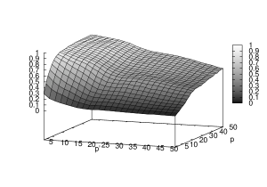
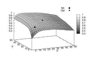
Figure 5: $\widetilde{U}(p^{\prime},p)$ for CSMA/CA for $5$ nodes without(left) and with(right) coalitions

Our tool detected a trivial NE UnitBackoff=0, see the plot at Fig. 5 (left) for an illustration. It means that a selfish node will always try to transmit as soon as possible by choosing UnitBackoff=0. This coincides with the results of [10] obtained for IEEE 802.11 CSMA/CA protocol. Intuitively, it is always profitable to transmit as soon as possible since if a selfish node will retransmit just after the collision, the rest (honest) nodes will probably detect this during the Clear Channel Assessment procedure and they will not corrupt the retransmission of the selfish node.

Number of nodes in one coalition	1	2	3	4	5
$\delta$-relaxed NE strategy $p_{NE}$	11	8	15	25	28
Value of $\delta$	0.900	0.985	0.986	0.990	0.990
$\widetilde{U}(p_{NE},p_{NE})$	0.86	0.76	0.81	0.85	0.83
Symmetric optimal strategy $p_{opt}$	13	23	31	34	48
$\widetilde{U}(p_{opt},p_{opt})$	0.87	0.85	0.87	0.87	0.86
Time	1m08s	5m45s	7m62s	32m49s	57m59s

Table 2: Nash equilibrium (NE) and Symmetric optimal (Opt) strategies for CSMA/CA with coalitions

In order to illustrate our algorithm we also considered the situation when network nodes (game players) form coalitions. It can correspond to the situation when several network devices belong to the same user and it will not be profitable for the user if these devices compete with each other. The intuition is that players of the same coalition will not choose “always transmit” strategy because in this case they will disturb each other. This is confirmed by plot at Fig. 5 (right) and table 2, where we considered the case of two coalitions of the same size.

6 Related Work

The paper [20] is the first one that applies the concept of Nash Equilibrium to the analysis of Medium Access and power control games in slotted Aloha protocol. Later this approach has been applied to the most of the layers of a network stack: to the Physical [5, 20, 21], Medium Access [22, 10, 12, 16], Network [15, 26] and Application [9] layers.

Although our approach can be in principle applied to any network layer, it is particularly well suited for the random access Medium Access layer protocols, since such protocols possess probabilistic behavior (here we can use our Weighted Timed Automata semantics) and work in real-time. In this settings, our SMC-based approach extends the manual analytical approach, that can be complicated, error-prone and typically applied to slotted (discrete time) protocols only [12, 20]. On the other hand, our approach extends the simulation-based approach (for instance, [10]), since we formally describe a modeling formalism for which we can provide a confidence on the results.

Additionally, in our paper we use the expressive PWCTL logic to express the goals of the network nodes, and thus to define their utility functions with respect to time and energy constraints. This allows us to apply the same framework to the analysis of different protocols, while another approaches does not allow such a generalization.

Our experimental results extend those proposed in [20] from the slotted Aloha to the unslotted one. Up to our knowledge, we are also the first ones, who study coalitions between nodes in the IEEE 802.15.4 CSMA/CA protocol.

7 Conclusions

In this paper we have presented a methodology to apply statistical model checking to search for a Nash equilibrium on different types of networks. Experiments demonstrate the maturity of our technique and shows that it can be applied in principle to more complex problems. The technique avoids analytical analysis of the model and contrary to pure simulation-based techniques, ours provides statistical confidence on its results. As future work we will extend the language of our tool to be able to apply it to other domains such as biological systems.

References

- [1]
- [2] Parosh Abdulla, Giorgio Delzanno, Othmane Rezine, Arnaud Sangnier & Riccardo Traverso (2011): On the Verification of Timed Ad Hoc Networks. In: Proceedings of the 9th International Conference on Formal Modeling and Analysis of Timed Systems (FORMATS’11), Lecture Notes in Computer Science , Springer, 10.1007/978-3-642-24310-3_18.
- [3] Norman Abramson (1970): The Aloha system: another alternative for computer communications. In: Proceedings of the November 17-19, 1970, fall joint computer conference, AFIPS ’70 (Fall), ACM, New York, NY, USA, pp. 281–285, 10.1145/1478462.1478502.
- [4] ZigBee Alliance (2005): ZigBee specification 1.0.
- [5] Eitan Altman, Nicolas Bonneau, Merouane Debbah & Giuseppe Caire (2005): An evolutionary game perspective to Aloha with power control. In: ITC 19, 19th International Teletraffic Congress, August 29 - September 2, 2005.
- [6] Rajeev Alur, Salvatore La Torre & George J. Pappas (2001): Optimal Paths in Weighted Timed Automata. In: HSCC’01, Springer, pp. 49–62, 10.1016/j.tcs.2003.10.038.
- [7] Gerd Behrmann, Ansgar Fehnker, Thomas Hune, Kim Guldstrand Larsen, Paul Pettersson, Judi Romijn & Frits W. Vaandrager (2001): Minimum-Cost Reachability for Priced Timed Automata. In: HSCC, pp. 147–161.
- [8] Patricia Bouyer, Kim Guldstrand Larsen & Nicolas Markey (2008): Model Checking One-Clock Priced Timed Automata. Logical Methods in Computer Science 4(2), 10.2168/LMCS-4(2:9)2008.
- [9] Levente Buttyan & Jean-Pierre Hubaux (2008): Security and Cooperation in Wireless Networks. Cambridge University Press, Cambridge.
- [10] Mario Cagalj, Saurabh Ganeriwal, Imad Aad & Jean-Pierre Hubaux (2004): On Cheating in CSMA/CA Ad Hoc Networks. Technical Report, Proc. IEEE INFOCOM 2005.
- [11] Franck Cassez & Kim Guldstrand Larsen (2000): The Impressive Power of Stopwatches. In: CONCUR, pp. 138–152, 10.1007/3-540-44618-4_12.
- [12] Johannes Dams, Thomas Kesselheim, & Berthold Vocking (2011): Transmission Probability Control Game with Limited Energy. In: IEEE DySPAN, to appear, 10.1109/DYSPAN.2011.5936232.
- [13] Alexandre David, Kim G. Larsen, Axel Legay, Marius Mikucionis, Danny Poulsen, Jonas van Vliet & Zheng Wang (2011): Statistical Model Checking for Networks of Priced Timed Automata. In: Proceedings of Formal Modeling and Analysis of Timed Systems, LNCS, Aalborg, pp. 80–96, 10.1007/978-3-642-24310-3.
- [14] Alexandre David, Kim G. Larsen, Axel Legay, Marius Mikucionis & Zheng Wang (2011): Time for Statistical Model Checking of Real-time Systems. In: Proceedings of the 23rd International Conference on Computer Aided Verification (CAV), LNCS, Springer Verlag, pp. 349–355, 10.1007/978-3-642-22110-1_27.
- [15] Mark Felegyhazi, Student Member, Jean pierre Hubaux, Senior Member & Levente Buttyan (2006): Nash Equilibria of Packet Forwarding Strategies in Wireless Ad Hoc Networks. IEEE Transactions on Mobile Computing 5, 10.1109/TMC.2006.68.
- [16] Abdorasoul Ghasemi & Karim Faez (2008): A nash power-aware MAC game for ad hoc wireless networks. In: PIMRC, IEEE, pp. 1–5, 10.1109/PIMRC.2008.4699511.
- [17] Ehud Kalai (1991): Game theory: Analysis of conflict : By Roger B. Myerson, Harvard Univ. 568 pp. Games and Economic Behavior 3(3).
- [18] Kim G. Larsen, Paul Pettersson & Wang Yi (1997): Uppaal in a Nutshell. Int. Journal on Software Tools for Technology Transfer 1(1–2), pp. 134–152, 10.1007/s100090050010.
- [19] Axel Legay & Benoît Delahaye (2010): Statistical Model Checking : An Overview. CoRR abs/1005.1327, 10.1007/978-3-642-16612-9_11.
- [20] A. B. Mackenzie & S. B. Wicker (2001): Game theory and the design of self-configuring, adaptive wireless networks. Communications Magazine, IEEE 39(11), pp. 126–131, 10.1109/35.965370.
- [21] J. Neel, R. Menon, A. MacKenzie & J. Reed (2005): Using game theory to aid the design of physical layer cognitive radio algorithms. In: Conf. on Economics, Technology and Policy of Unlicensed Spectrum.
- [22] P Nuggehalli, M Sarkar, K Kulkarni & R Rao (2008): A Game-Theoretic Analysis of QoS in Wireless MAC. In: INFOCOM 2008. The 27th Conference on Computer Communications. IEEE, pp. 1903–1911, 10.1109/INFOCOM.2008.254.
- [23] IEEE Computer Society (2003): Wireless Medium Access Control (MAC) and Physical Layer (PHY) Specifications for Low-Rate Wireless Personal Area Networks (WPANs).
- [24] V. Srivastava, J. Neel, A.B. Mackenzie, R. Menon, L.A. Dasilva, J.E. Hicks, J.H. Reed & R.P. Gilles (2005): Using game theory to analyze wireless ad hoc networks. Communications Surveys Tutorials, IEEE 7(4), pp. 46 – 56, 10.1109/COMST.2005.1593279.
- [25] Hakan L. S. Younes (2005): Verification and Planning for Stochastic Processes with Asynchronous Events. Ph.D. thesis, Carnegie Mellon University.
- [26] Irfan Zakiuddin, Tim Hawkins & Nick Moffat (2005): Towards A Game Theoretic Understanding of Ad-Hoc Routing. Electronic Notes in Theoretical Computer Science 119(1), pp. 67 – 92, 10.1016/j.entcs.2004.07.009.