3-D Monte Carlo radiative transfer calculation of resonance line formation in the inhomogeneous expanding stellar wind

Abstract

We study the effects of optically thick clumps, non-void inter-clump medium, variation of the onset of clumping, and velocity dispersion inside clumps on the formation of resonance lines. For this purpose we developed a full 3-D Monte Carlo Radiative Transfer (MCRT) code that is able to handle 3-D shapes of clumps and arbitrary 3-D velocity fields. The method we developed allows us to take into account contributions from density and velocity wind inhomogeneities to the total opacity very precisely. The first comparison with observation shows that 3-D density and velocity wind inhomogeneities have a very strong influence on the resonance line formation, and that they have to be accounted for in order to obtain reliable mass-loss rate determinations.

¹Astronomický ústav AV ČR, Fričova 298, 251 65 Ondřejov, Czech Republic

²Matematicko-fyzikální fakulta UK, Ke Karlovu 3, 121 16 Praha 2

³Institut für Physik und Astronomie, Universitätsstandort Golm, Karl-Liebknecht-Str. 24/25, Potsdam, Germany

1 Introduction

There is a lot of observational and theoretical evidence that the winds of hot stars are inhomogenoues. Stochastic variable structures in the He ii $\lambda$ $4686\AA$ emission line in $\zeta$ Pup were revealed by Eversberg et al. (1998), and explained as an excess emission from the wind clumps. Markova et al. (2005) investigated the $\mathrm{H}\alpha$ line-profile variability for a large sample of O-type supergiants. They concluded that the properties of this variability can be explained by a wind model consisting of clumps.

Understanding of clumping is a prerequisite to obtain correct mass-loss rates from modeling the stellar spectra (see Fullerton et al. 2006; Bouret et al. 2005; Puls et al. 2006; Oskinova et al. 2007).

A possible way how to study wind clumping is to use simplifications. The approximate treatment of clumping is usually based on the “microclumping” (clumps are optically thin at all frequencies) or “macroclumping” (clumps may be optically thick for certain wavelengths) approaches. Common additional assumptions are the void interclumped medium (ICM) and the monotonic velocity field. The enhancement of the density inside clumps is usually described by the so called “clumping factor” $D$.

In the most recent studies of Sundqvist et al. (2010, 2011) it was shown that the detailed density structure, non-monotonic velocity field, and the ICM are all important for the line formation in the massive hot star winds. In order to be able to study the 3-D nature of wind clumping and to take into account all properties of wind clumping mentioned here, we developed a realistic full 3-D MCRT code (Šurlan et al., in preparation). Here we present the basic effects of the different clump properties on the resonance line formation and present the first preliminary comparison with observation.

2 The clumped wind model

Our wind model is grid-less and does not require any symmetry. Instead of using a predefined grid, we introduce an adaptive integration step $\Delta r$. First we create a snapshot of clumps inside the wind and then we follow photons along their paths using the Monte Carlo approach. The photon frequencies are expressed in the local co-moving frame. All distances are expressed in units of the stellar radius ($R_{\ast}$).

The velocity field can be arbitrary in our wind model. However, here we assumed a radial monotonic velocity $\varv_{r}$ field and the standard $\beta$-velocity law for the underlying smooth wind ($\varv_{r}=\varv_{\beta}$). The velocity inside clumps $\varv_{c}$ is expressed as

$$\varv_{c}(r)=\varv_{\beta}(r^{\mathrm{c}}_{i})-\varv_{\mathrm{dis}}(r)\,\frac{r-r^{\mathrm{c}}_{i}}{l_{i}},$$ (1)

where $\varv_{\mathrm{dis}}(r)=m\,\varv_{\beta}(r)$ describes the velocity dispersion using the deviation parameter $m$ ($0<m\leq 1$). The monotonic velocity at the position $r^{\mathrm{c}}_{i}$ is $\varv_{\beta}(r^{\mathrm{c}}_{i})$, and $l_{i}$ and $r^{\mathrm{c}}_{i}$ are the radius and the absolute position of the center of the $i$-th clump, respectively.

The opacity of the wind is calculated using the parameterization given by Hamann (1980),

$$\chi(r)=\frac{\chi_{0}}{r^{2}\frac{\varv_{r}}{\varv_{\infty}}}\,\phi_{x};\quad\phi_{x}=\frac{1}{\sqrt{\pi}}\,e^{-x^{2}},$$ (2)

where $\chi_{0}$ is the opacity parameter that corresponds to the line strength, $\varv_{\infty}$ is the terminal velocity of the wind, and $\phi_{x}$ is the absorption profile, which depends on the dimensionless frequency $x=\left({\nu}/{\nu_{0}}-1\right){c}/{\varv_{D}}$, where $\varv_{D}$ is the Doppler-broadening velocity which comprises both the thermal broadening and microturbulence. The ionisation is assumed to be constant.

For simplicity we assume a spherical shape of the clumps with a radius that varies with the distance $r$ from the star, $l=l(r)$. A clump radius is determined using the clump separation parameter $L_{0}$ as

$$l(r)=l_{0}\,\sqrt[3]{r^{2}\,\varw(r)};\quad\text{where}\quad l_{0}=L_{0}\sqrt[3]{\frac{3}{4\pi D}},$$ (3)

$\varw(r)=\varv_{r}/\varv_{\infty}$ is the velocity in the units of the terminal speed $\varv_{\infty}$, and $D$ is the clumping factor. The average clump separation $L$ is also depth dependent and given as $L(r)=L_{0}\sqrt[3]{r^{2}\,\varw(r)}$. The density inside clumps is assumed to be by the clumping factor $D$ higher than the smooth wind density. In the first approximation, $D$ is assumed to be independent on $r$ and given by

$$D=\frac{L^{3}(r)}{\frac{4\,\pi}{3}l^{3}(r)},\quad D\geq 1.$$ (4)

The ICM density is determined by the interclump density parameter $d$ which is also assumed to be depth independent and $0\leq d<1$. If the factor $d=0$, the ICM is void, otherwise the ICM is rarefied by the factor $d$ compared to the smooth wind density. For the case of dense clumps and void ICM, all the mass of the wind is put into clumps, and the volume filling factor is $f_{V}=1/D$. For the case of dense clumps and non-void ICM, the mass of the wind is distributed between clumps and ICM and it follows that $f_{V}=(1-d)/(D-1)$.

The total number of the clumps is determined by the condition of the mass conservation inside the wind. Clumps are created one by one and when the total volume of created clumps ($V_{\mathrm{cl}}$) is larger than the total volume of the wind ($V_{w}$) multiplied by $f_{V}$, i.e. if $V_{\mathrm{cl}}\geq f_{V}V_{w}$, then the number of created clumps represents the total number of clumps in our snapshot clump distribution.

3 Effect of different clump properties

By varying the model parameters we examined how macroclumping (defined by $L_{0}$ and $D$), non monotonic velocity field ($\varv_{\mathrm{dis}}$), non void ICM ($d$), and onset of clumping ($r_{\mathrm{cl}}$) may influence weak ($\chi_{0}=0.5$), intermediate ($\chi_{0}=50$), and strong ($\chi_{0}=500$) resonance line profiles. Calculations are performed assuming $\sim 10^{4}$ clumps inside wind, which corresponds to $L_{0}=0.5$ for the wind with $r=10$. The clumping factor is set to $D=10$. The Doppler-broadening velocity is $\varv_{D}=50\,\mathrm{km}\,\mathrm{s}^{-1}$. A snapshot of distribution of the clumps is shown in Fig. 1, upper right panel.

The first set of line profiles (C1 in Fig. 1) is calculated assuming that clumping starts at the surface of the star ($r_{\mathrm{cl}}=1$) with void ICM ($d=0$), and monotonic velocity field ($\varv_{\mathrm{dis}}=\varv_{\beta}$). The weak (upper left panel), intermediate (lower left panel), and strong (lower right panel) lines show strong line strength reduction compared to the smooth wind (full lines). If the wind is clumped, more photons can escape through “holes” between clumps. This leads to lower effective opacities, and, consequently, less absorption. The line strength reduction depends on the number of clumps in the wind. The absorption dip close to $\varv_{\infty}$ is caused by lower probability of photon escape through lower number of velocity “holes”.

In order to investigate how the onset of clumping influences line profiles, we calculated the second set of line profiles (C2 in Fig. 1) assuming that clumping is only above $r_{\mathrm{cl}}=1.3$. Other model parameters are the same as for the first set of line profiles calculations. A very strong and broad absorption near the line centers appears. It is due to a higher absorption of the smooth part of the wind, which is in the region $1<r<r_{\mathrm{cl}}$. Such deep absorption is not observed and it disappears if clumping starts closer to the wind base (perhaps even from the surface of the star) or if the ICM is sufficiently dense. The weak line almost reproduces the smooth wind model in this case. For a small value of $\chi_{0}$, the clumps are optically thin and they have a very small influence on the line profile compared to the smooth wind.

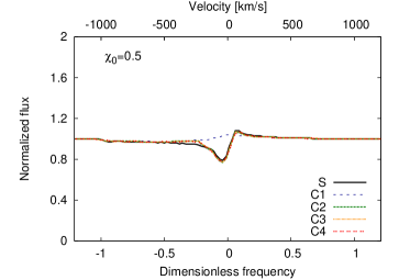
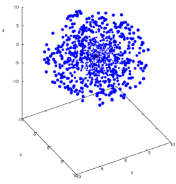
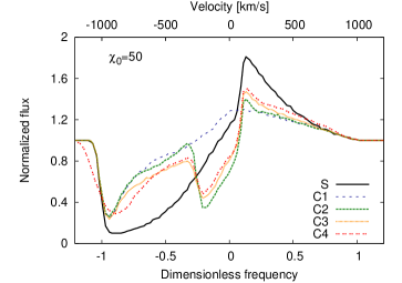
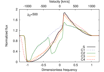
Figure 1.: Line profiles for weak (upper left panel), medium (lower left panel), and strong (lower right panel) lines for the clump distribution in the upper right panel. S – the smooth model; C$n$ denotes the clumped models – C1 ($r_{\mathrm{cl}}=1$), C2 ($r_{\mathrm{cl}}=1.3$), C3 ($r_{\mathrm{cl}}=1.3$, $d=0.05$), C4 ($r_{\mathrm{cl}}=1.3$, $d=0.05$, $\varv_{\mathrm{dis}}=0.2\,\varv_{\beta}$).

Varying the ICM density parameter $d$, a significant impact on the line profiles was found, especially on strong lines. Keeping the same parameters as for the second set of line profile calculation, but choosing $d=0.05$ we calculated the third set of line profiles (C3 in Fig. 1). While the weak line is unaffected, the intermediate and strong ones show an increase of absorption in the blue edge of the line and a decrease of absorption near the centre of the line. The degree of the line saturation depends on the ICM density. For a particular value of $d$, saturation of strong lines and desaturation of the intermediate lines can be achieved.

Taking into account the non-monotonic velocity field, an absorption at velocities higher than $\varv_{\infty}$ appears. Setting $\varv_{\mathrm{dis}}=0.2\,\varv_{\beta}$ and keeping other model parameters the same as for the third set of line profiles, we calculated the fourth set of line profiles (C4 in Fig. 1). The higher $\varv_{\mathrm{dis}}$, the larger is the velocity span of clumps, and, consequently, there are more velocity overlaps (the “holes” in the velocity field are smaller) and the probability of the photon escape is lower.

4 Comparison with observations

As the first attempt to compare with observations, we try to fit the P v doublet of $\zeta$ Pup observed by the copernicus satellite (thin line in Fig. 2). As the terminal velocity of $\zeta$ Pup we adopt $\varv_{\infty}=2250\,\mathrm{km}\,\mathrm{s}^{-1}$, and the value of $\beta=0.9$. The synthetic spectrum of the smooth and clumped wind models are calculated. The model parameters are chosen to fit the observed spectrum best. It can be seen that the predicted unclumped (smooth) P-Cygni profile (full line with crosses) of P v is much stronger than the observed one (thin full line). However, the synthetic spectrum for the clumped model (thick full line) fits the strength of the observed line very well. Therefore, using the unclumped model can lead to underestimating the empirical mass-loss rates. These results are consistent with Oskinova et al. (2007) and Sundqvist et al. (2010, 2011).

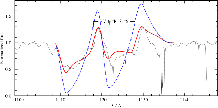
Figure 2.: Comparison of line profiles calculated using different wind models with copernicus observations (thin full line).The unclumped wind model is shown by the full line with crosses, while clumped model is shown by the thick full line.

5 Conclusions

Using our 3-D Monte Carlo Radiative Transfer code, we investigate the influence of the 3-D stellar wind clumping on the resonance line formation. Our results show that clumping may significantly reduce the strength of lines and, if not included, may lead to a wrong mass-loss rate determination. The 3-D wind nature, the onset of clumping, non void ICM, and non-monotonic velocity field are all important model ingredients. Our models allow to obtain these parameters from the comparison between model and observed lines, and thus gain deep insight in the structure of stellar winds, and obtain reliable mass-loss rate measurements.

Acknowledgments

This research was supported by grants GA ČR 205/08/H005, GA ČR 205/08/0003, and GA UK 424411.

References

- Bouret et al. (2005) Bouret, J.-C., Lanz, T., & Hillier, D. J. 2005, A&A, 438, 301
- Eversberg et al. (1998) Eversberg, T., Lepine, S., & Moffat, A. F. J. 1998, ApJ, 494, 799
- Fullerton et al. (2006) Fullerton, A. W., Massa, D. L., & Prinja, R. K. 2006, ApJ, 637, 1025
- Hamann (1980) Hamann, W.-R. 1980, A&A, 84, 342
- Markova et al. (2005) Markova, N., Puls, J., Scuderi, S., & Markov, H. 2005, A&A, 440, 1133
- Oskinova et al. (2007) Oskinova, L. M., Hamann, W.-R., & Feldmeier, A. 2007, A&A, 476, 1331
- Puls et al. (2006) Puls, J., Markova, N., Scuderi, S., et al. 2006, A&A, 454, 625
- Sundqvist et al. (2010) Sundqvist, J. O., Puls, J., & Feldmeier, A. 2010, A&A, 510, A11
- Sundqvist et al. (2011) Sundqvist, J. O., Puls, J., Feldmeier, A., & Owocki, S. P. 2011, A&A, 528, A64