The Stellar Halos of Massive Elliptical Galaxies

Abstract

We use the Mitchell Spectrograph (formerly VIRUS-P) on the McDonald Observatory 2.7m Harlan J. Smith Telescope to search for the chemical signatures of massive elliptical galaxy assembly. The Mitchell Spectrograph is an integral-field spectrograph with a uniquely wide field of view ($107\times 107$ sq arcsec), allowing us to achieve remarkably high signal-to-noise ratios of $\sim 20-70$ per pixel in radial bins of $2-2.5$ times the effective radii of the eight galaxies in our sample. Focusing on a sample of massive elliptical galaxies with stellar velocity dispersions $\sigma_{\ast}$$>150$ km s^-1, we study the radial dependence in the equivalent widths (EW) of key metal absorption lines. By twice the effective radius, the Mg$b$ EWs have dropped by $\sim 50\%$, and only a weak correlation between $\sigma_{\ast}$ and Mg$b$ EW remains. The Mg$b$ EWs at large radii are comparable to those seen in the centers of elliptical galaxies that are $\sim$ an order of magnitude less massive. We find that the well-known metallicity gradients often observed within an effective radius continue smoothly to $2.5R_{e}$, while the abundance ratio gradients remain flat. Much like the halo of the Milky Way, the stellar halos of our galaxies have low metallicities and high $\alpha$-abundance ratios, as expected for very old stars formed in small stellar systems. Our observations support a picture in which the outer parts of massive elliptical galaxies are built by the accretion of much smaller systems whose star formation history was truncated at early times.

1 Introduction

Elliptical galaxies are comprised of mostly old stars, contain little gas or dust, and show very tight scaling relations between their sizes, central surface brightnesses, and stellar velocity dispersions (the Fundamental Plane, e.g., Djorgovski & Davis, 1987; Dressler et al., 1987). Despite their apparent simplicity, observations of elliptical galaxies continue to surprise and confound us. Their central stellar populations suggest that the most massive elliptical galaxies formed their stars rapidly and early (e.g., Faber, 1973; Thomas et al., 2005). And yet, evidence for dramatic size evolution has emerged, such that elliptical galaxies at $z\approx 1$ were apparently a factor of $\sim 2$ smaller at fixed mass than they are today (e.g., Trujillo et al., 2006; van Dokkum et al., 2008; van der Wel et al., 2008; Cimatti et al., 2008; Damjanov et al., 2009; Cassata et al., 2010). It is, of course, extremely challenging to measure galaxy sizes at high redshift (e.g., Hopkins et al., 2009; Saracco et al., 2010), but evidence continues to mount that the size evolution is real (e.g., Newman et al., 2011; Brodie et al., 2011; Papovich et al., 2011).

The most common scenario to explain the dramatic size growth in elliptical galaxies at late times invokes minor merging that can make galaxies fluffier without adding very much mass (e.g., Gallagher & Ostriker, 1972; Boylan-Kolchin & Ma, 2007; Naab et al., 2007, 2009; Newman et al., 2011). Naively, late-time merging with small systems would wash out the well-established scaling relations between stellar velocity dispersion ($\sigma_{\ast}$) and stellar population properties observed in local elliptical galaxies, such as the Mg$b$-$\sigma_{\ast}$ relation (e.g., Bender et al., 1993). Furthermore, stellar population studies of local elliptical galaxies clearly find that the stars in the most massive elliptical galaxies were formed earliest ($z>2$) and fastest ($<$ Gyr), while lower-mass systems have more extended formation histories and later formation times (e.g., Thomas et al., 2005). From the tight color-magnitude relation alone it is hard to support much late-time star formation (or the addition of more metal-poor stars, e.g., Bower et al., 1992).

The tension between the tight scaling relations of elliptical galaxies and their apparent puffing up from late-time merging is alleviated if the stars added at late times are deposited at large radius. The vast majority of stellar population work is heavily weighted towards the very luminous central component of these galaxies, usually well within the half-light radius ($R_{e}$; e.g., Faber, 1973; Rawle et al., 2008; Graves et al., 2009; Kuntschner et al., 2010). Recently, thanks to the Sloan Digital Sky Survey (SDSS; York et al., 2000), very large samples of elliptical galaxies are now available for examining color gradients (e.g., Zibetti et al., 2005; Tortora et al., 2010; Suh et al., 2010; Gonzalez-Perez et al., 2011). With few exceptions (e.g., Rudick et al., 2010), these observations have not extended much beyond the effective radius. To fully exploit the fossil record to understand the assembly of elliptical galaxies, we ought to look for radial changes in the stellar population, particularly beyond $R_{e}$.

The study of the radial dependence of chemical composition in elliptical galaxies has a long history. Imaging studies of elliptical galaxy colors date back to de Vaucouleurs (1961). Since then, there have been many studies made of the radial color gradients in elliptical galaxies (e.g., Tifft, 1969; Wirth & Shaw, 1983; Eisenhardt et al., 2007). The summary presented in Strom & Strom (1978) remains accurate today; elliptical galaxies are bluer at large radii, most likely due to a decline in metallicity (Spinrad, 1972; Strom et al., 1976). However, with photometry alone it is difficult to precisely disentangle the well-known degeneracies between age and metallicity (e.g., Worthey, 1994). Many spectroscopic surveys have looked at the gradients in the equivalent widths (EW) of key metal lines that can break these degeneracies (e.g., Spinrad & Taylor, 1971; Faber et al., 1977; Gorgas et al., 1990; Fisher et al., 1995; Mehlert et al., 2003; Ogando et al., 2005; Brough et al., 2007; Baes et al., 2007; Annibali et al., 2007; Sánchez-Blázquez et al., 2007; Rawle et al., 2008; Kuntschner et al., 2010; Weijmans et al., 2009). Roughly speaking, spectroscopic work confirms the overall conclusions from imaging studies. Metallicity dominates the color changes, decreasing outwards by 0.1-0.5 dex per decade in radius. In general there is no strong evidence for age gradients (although see Baes et al. for an alternate view).

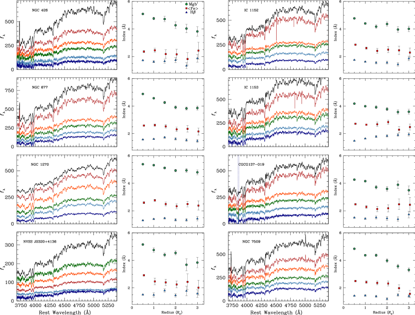
Figure 1: Spectra (left, middle) and index equivalent widths (right) for our sample. Left, middle: Spectra are plotted in elliptical annuli of (from top to bottom) $0-0.5R_{e}$, $0.5-1R_{e}$, $1-1.5R_{e}$, $1.5-2R_{e}$, and $2-2.5R_{e}$ (see Table 1). Units are $10^{-17}$erg s^-1 cm^-2 Å^-1, but the spectra have been offset for clarity. The sky feature in CGCG137$-019$ is highlighted with a dotted vertical line. Right: We show the Mg$b$ index (green circles), the $\langle$Fe$\rangle$ index, which is the average of the Fe 5270 and Fe 5335 indices (red squares), and the H$\beta$ index (blue triangles) in Å. Error bars are derived via Monte Carlo simulations as described in §4.2.1. The $\langle$Fe$\rangle$ index is offset slightly in radius for clarity.

Spectroscopic surveys can track more than just metallicity and age. They can also study the relative abundances of individual elements. In particular, the $\alpha$ elements (e.g., Mg, C, O, N) are formed in Type II supernova explosions, while the Fe-peak elements (Fe, Cr, Mn) are formed predominantly in Type Ia supernovae, and are thus produced with a temporal lag from the peak of star formation. The relative quantity of $\alpha$ to Fe-peak elements provides a star-formation timescale, with enhanced $\alpha$/Fe ratios pointing to rapid time-scales of star formation. Elliptical galaxies display a strong trend of increasing $\alpha$/Fe abundance with increasing mass or stellar velocity dispersion (e.g., Faber, 1973; Terlevich et al., 1981; Worthey et al., 1992) although see also Kelson et al. (2006). It is therefore thought that the most massive elliptical galaxies formed their stars rapidly and at $z\mathrel{\hbox{\hbox to0.0pt{\hbox{\lower 4.0pt\hbox{$\sim$}}\hss}\hbox{\raise 2.0pt\hbox{$>$}}}}2$ (e.g., Thomas et al., 2005). Thus far, no strong gradients in $\alpha$/Fe ratios have been detected at large radii (e.g., Kuntschner et al., 2010; Spolaor et al., 2010, and references therein).

A few studies have managed to probe stellar populations in elliptical galaxies beyond the effective radius. It is very hard to achieve the required signal-to-noise at large radii with long-slit spectroscopy since the area subtended on the sky is small and the sky level is factors of several brighter than the signal (e.g., Kelson et al., 2002; Sánchez-Blázquez et al., 2007). Integral-field unit (IFU) spectroscopy provides two-dimensional information, and coadding the signal in annuli strongly boosts the signal relative to the sky. A handful of studies thus far have used IFUs with smaller fields of view, and either tile the instrument at large radius (e.g., Weijmans et al., 2009) or focus on the central regions of the galaxy (Rawle et al., 2008; Kuntschner et al., 2010). In this work, we exploit the $4\farcs 2$ diameter fibers and $107\times 107$″ field of view of the Mitchell Spectrograph to study the spatial variation in age, metallicity, and abundance ratio gradients for eight massive early-type galaxies. Our increased leverage on stellar populations in the galaxy outskirts will allow us to put new constraints on the assembly of massive elliptical galaxies at late times.

In §2 we describe the sample and in §3 we describe the instrument and data reduction. The analysis is described in §4. Those most interested in results can focus on §5 and the subsequent discussion in §6. We summarize and conclude in §7. When needed, we use the standard concordance cosmology of Dunkley et al. (2009).

2 Sample

We start with a small pilot sample of eight galaxies as a proof of concept that the Mitchell Spectrograph is well-suited to this work (Table 1, Figure 1). The sample selection is not ideal, and we do not make claims of its completeness or uniformity, since the galaxies were selected with other science goals in mind. In short, we selected galaxies with red colors ($u-r>2.2$; Strateva et al., 2001), stellar velocity dispersions that are larger than the instrumental resolution of the Mitchell Spectrograph ($\sigma_{\ast}$$>150$ km s^-1; as measured by the SDSS pipeline) and redshifts in the narrow range

$0.015<z<0.02$ (85 Mpc, for a scale of 0.4 kpc per ″). We examine all of the candidates and remove obvious edge-on disk galaxies, but have made no formal morphology cut. Thus there are two S0s in the final sample (CGCG137$-$019 and IC 1153). We also make no selection on environment. However, in the sample there is a cluster galaxy (NGC 1270; Miller & Owen, 2001), two brightest group galaxies (NGC 677 and NGC 426; Berlind et al., 2006), two that belong to the same group (IC 1152 and IC 1153; White et al., 1999) and the rest are in lower density environments. Using our stellar velocity dispersion measurements, simple dynamical mass estimates for the galaxies range from $8\times 10^{10}-3\times 10^{11}$ $M_{\odot}$, with only one below $10^{11}$ $M_{\odot}$. Based on the mass function from Bell et al. (2003), they range from one to four times $M^{*}$ for ellipticals.

3 Observations and Data Reduction

The observations were obtained over two runs, one in Sept 2010 (including the bulk of the galaxies) and the other in June 2011 (IC 1152, IC 1153; Table 1). We used the George and Cynthia Mitchell Spectrograph (the Mitchell Spectrograph, formerly VIRUS-P; Hill et al., 2008a) on the 2.7m Harlan J. Smith telescope at McDonald Observatory. The Mitchell Spectrograph was built as a prototype for the VIRUS spectrograph that will soon be deployed on the Hobby-Eberly Telescope to perform a dark energy experiment (HETDEX; Hill et al., 2008b). Each of the 246 fibers subtends $4\farcs 2$ and are assembled in an array similar to Densepak (Barden et al., 1998) with a 107″$\times$107″ field of view and a one-third filling factor. The Mitchell Spectrograph has performed a very successful search for Ly$\alpha$ emitters (Adams et al., 2011; Finkelstein et al., 2011; Blanc et al., 2011) and has become a highly productive tool to study spatially resolved kinematics and stellar populations in nearby galaxies (Blanc et al., 2009; Yoachim et al., 2010; Murphy et al., 2011; Adams et al., 2012).

We used the low-resolution blue setting of the Mitchell Spectrograph. Our wavelength range spans 3550-5850Å with an average spectral resolution of $5\,$Å FWHM. This resolution delivers a dispersion of $\sim$ $1.1\,$Å pixel^-1 and corresponds to $\sigma_{\ast}$ $\approx 150$ km s^-1 at $4300\,$Å, our bluest Lick index. Each galaxy was observed for a total of $\sim 2$ hours with one-third of the time spent at each of three dither positions to fill the field of view. Initial data reduction was accomplished using the custom code Vaccine (Adams et al., 2011; Murphy et al., 2011). We briefly review the steps of the pipeline here, but refer the interested reader to the previous papers for more detailed discussion. Initial overscan and bias subtraction are performed first on all science and calibration frames. All co-additions of data and calibration frames are performed with the biweight estimator (Beers et al. 1990). Twilight flats are used to construct a trace for each fiber, which takes into account curvature in the spatial direction. We employ a routine similar to that proposed by Kelson (2003) to avoid interpolation during this step. Thanks to this special care, correlated errors are avoided and it is possible to track the S/N in each pixel through the remainder of the reductions. Knowing the S/N in each pixel enables deeper limits in detection experiments such as those performed by Adams et al. (2011). All subsequent operations are conducted in the new trace coordinate system within a cross-dispersion aperture of 5 pixels.

To correct for curvature in the spectral direction, a wavelength solution is derived for each fiber based on arcs taken both at the start and end of the night. Gaussian fits to known arc lines are fit with a fourth-order polynomial to derive a complete wavelength solution for each fiber. The typical rms residual variations about this best-fit fourth-order polynomial are $0.08\,$Å for the Sept 2010 data and $0.04\,$Å for our June 2011 data. A heliocentric correction is then calculated for each science frame.

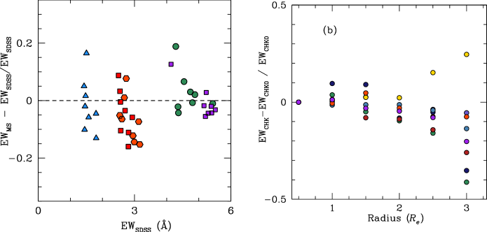
Figure 2: a: Comparison between the Lick indices measured from the SDSS spectrum and our central 0.5$R_{e}$ bin for H$\beta$ (blue triangles), the G-band at $4300\,$Å (purple squares), the Mg$b$ triplet (green circles), the Fe 5270 line (red squares), and the Fe 5335 line (red hexagons). Fractionally, the two sets of indices agree within $3\%$ of each other, while the mean deviation $\langle({\rm EW}_{\rm MS}-{\rm EW}_{\rm SDSS})/{\rm EW}_{\rm SDSS}\rangle=-0.02\pm 0.08$. The $\langle$Fe$\rangle$ index is systematically offset to lower values in our spectra by enough to introduce significant systematic offsets in the inferred metallicity. b: Fractional change in the EW of Ca H+K as a function of radius for all galaxies in the sample. Each color represents a different source. Note that the fluctuations between $0<$R${}_{e}<2$ are within $10\%$, which is both the typical error in these measurements and the level at which Ca H+K is expected to vary due to real changes in stellar population. It is only in the outermost bin (2.5-3$R_{e}$) that we see systematic effects begin to artificially lower the EW in some objects. The yellow points that rise at large radii correspond to CGCG137$-019$, which was observed at twilight and has imperfect sky subtraction.

Next, a flat field is constructed from the twilight flats taken at both the start and end of the night. Variations in temperature never exceeded 2 C for any of our observing nights and the stability of the flat field has been shown to be $<0.1$ pixels under these conditions (Adams et al., 2011). As the twilight flats contain solar spectrum, we generate a model of this component by employing a bspline fitting routine (Dierckx, 1993). A boxcar of 51 fibers is employed to model the solar spectrum that effectively removes all cosmic rays, continuum sources, and variations in the flat field, in order to isolate the solar spectrum. The spatial and spectral curvature are leveraged here in order to supersample the solar spectra within the boxcar. This supersampled bspline fit to the solar spectra within each fiber is then divided into the original flat. What remains are the flat field effects that we want to capture: variations in the individual pixel response, in the relative fiber-to-fiber variation, and in the cross-dispersion profile shape for every fiber. This flat field is then applied to all of the science frames.

The next step is sky subtraction. Unlike some instruments (e.g., Sauron; Bacon et al., 2001), the Mitchell Spectrograph does not have dedicated sky fibers. Instead, we observed off-galaxy sky frames with a sky-object-object-sky pattern, with five minute exposure times on sky and twenty minute object exposures. The sky nods are processed in the same manner as the science frames described above. In order to create a sky frame we give an equal weighting of two to each sky nod, then coadd them to achieve an equivalent exposure time as the science frames. The advantage of sky nods is the high S/N we achieve in our sky estimate, based on the large number of fibers in the IFU. The disadvantage is that we sample the sky at a different time than the science frames and are thus subject to temporal variations in the night sky, particularly at twilight. However, by varying the weights given to each sky nod we are able to explore possible systematics due to sky variability. For all lines measured, no EW value changes by more than $0.08\,$Å due to temporal sky changes, even at the largest radii considered in this paper. We give the details and return to possible systematics related to sky subtraction in §4.2.1. Once the sky subtraction is complete, cosmic rays are identified and masked.

We use software developed for the VENGA project (Blanc et al., 2009) for flux calibration and final processing. We observe flux calibration stars each night using a six-point dither pattern and derive a relative flux calibration in the standard way. Then we use tools developed by M. Song, et al. (in preparation) to derive an absolute flux calibration relative to the SDSS imaging. M. Song uses synthetic photometry on each fiber and scales it to match the SDSS $g-$band image of each field, with a median final correction of $\sim 20\%$. The correction exceeds $50\%$ only during a period of high cirrus in the second night of observing in Sept 2010, which affects NVSS J0320+4136 and NGC 426. Finally, all fibers are interpolated onto the same wavelength scale and combined.

3.1 Radial bins

We focus on spectra combined in elliptical annuli with a width of 0.5$R_{e}$. Since the effective radii of these galaxies are $\sim$ twice the fiber diameter of 4″, 0.5$R_{e}$ is roughly the scale of a single fiber. In all cases we use the de Vaucouleurs radius derived by the SDSS pipeline. Since we are averaging over such large physical areas on the sky, the exact measured $R_{e}$ should not impact the conclusions. We did experiment with using wider radial bins at large radius to extend further from the galaxy center. However, we did not boost the S/N appreciably in this way. Furthermore, we begin to be systematics limited at $\sim 3R_{e}$ (§4.2.1). The bins consist of 1-4 fibers at $0-0.5R_{e}$, increasing to 20-40 fibers at $2-2.5R_{e}$. The S/N per final coadded spectrum is shown in Table 2.

Since all of our galaxies by selection have SDSS spectra, we can test the wavelength dependence of the flux calibration by comparing the shape of the spectrum in the central fiber of the Mitchell Spectrograph with the SDSS spectrum. We find $\sim 5\%$ agreement in nearly all cases, with no more than $\sim 15\%$ differences at worst.

4 Analysis

Our ultimate goal is to derive the stellar population properties of the galaxies using the absorption line spectra. In principle, we can use full spectral synthesis techniques (e.g., Bruzual & Charlot, 2003; Coelho et al., 2007; Vazdekis et al., 2010), and exploit all the information available in the spectra. However, in practice, there are a number of hurdles, including imperfect flux calibration and systematic color effects, that make the model fitting sensitive in systematic ways to imperfections in our data. It is known that the models are not always able to fit the absorption line equivalent widths (e.g., Gallazzi et al., 2005), although see also Koleva et al. (2011). Since we are most interested in measuring changes in stellar population properties as a function of radius, we use line index measurements (e.g., Lick indices, Faber et al., 1985; Worthey et al., 1994). As most prior work on this subject has used similar methodology, we are in a good position to compare with the literature. Keep in mind that we are thus measuring the luminosity-weighted mean properties of the stellar population.

Another major uncertainty in these stellar population synthesis models comes from our relative ignorance of stellar spectral energy distributions for stars with very different metallicities and/or abundance ratio patterns than stars in our solar neighborhood. These modeling deficiencies impact our study directly, since elliptical galaxies tend to have higher metallicities and $\alpha$-abundance ratios than local stars. Lately, the problem has garnered substantial attention both from the point of view of full spectra synthesis (e.g., Coelho et al., 2007; Conroy & van Dokkum, 2011; Maraston & Stromback, 2011) and for Lick index inversion methods (Thomas et al., 2003; Schiavon, 2007; Vazdekis et al., 2010). We exploit these modern models, but note that our knowledge of the underlying stellar evolution remains imperfect.

4.1 Emission line contamination

Something like $80\%$ of elliptical galaxies contain low levels of ionized gas within an effective radius (Sarzi et al., 2010; Yan & Blanton, 2011). For our purposes, this emission serves only as a contaminant, as it fills in the absorption features that we are trying to measure. By far the strongest emission feature in our spectra is the [O II]$~{}\lambda\lambda 3726,3729$ line, but there are no absorption features of interest that are confused by [O II]. It is contamination from H$\beta$ and [O III]$~{}\lambda 5007$ that concerns us here. In order to correct for this low-level emission, we adapt the code pPXF+GANDALF developed by M. Sarzi (Sarzi et al., 2006) and M. Cappellari (Cappellari & Emsellem, 2004). pPXF performs a weighted fit to the galaxy continuum using spectral templates provided by the user, including a polynomial fit to the continuum and a Gaussian broadening to represent the intrinsic dispersion of the galaxy. From these fits we derive a measurement of the stellar velocity dispersion in each radial bin. GANDALF iteratively measures the emission and continuum features simultaneously, to achieve an unbiased measurement of both components. As templates, we use Bruzual & Charlot (2003) single-age stellar population models with $\sigma\approx 70$ km s^-1 resolution. In principle, we could use these fits to trace the stellar populations with radius, but for the reasons discussed above, we do not find this methodology robust.

In general, the emission-line EW is small compared to that of the absorption lines. The maximum contamination comes in the central fiber of NGC 7509 (which has high-ionization lines indicative of an accreting black hole at the center). However, note that our spectral resolution of $150$ km s^-1 is not necessarily high enough to resolve the emission lines.

We compare the fit to [O III] from the central pixel of the Mitchell spectra with the SDSS line fits at twice the resolution. The two fits agree within $\sim 30\%$ (range of $2-70\%$ differences). As a result of the weakness of the features and the low spectral resolution, we do not have strong constraints on the flux or line shape of these emission lines. We incorporate emission line subtraction into our error bar estimates as described below. While the emission-line gas is not the focus of this paper, we note that in a few cases the [O II] emission is observed to extend beyond $2R_{e}$. An analysis of this emission will be the focus of a different work.

Unfortunately, even very small corrections do lead to substantive changes in the inferred galaxy ages – $0.1\,$Å of H$\beta$ emission infill corresponds to an age difference of $\sim 1$ Gyr (Schiavon, 2007; Graves & Faber, 2010). Thus, we caution that the absolute ages derived here are uncertain at this level. In some cases, in fact, the small infill of the H$\beta$ lines by emission leads to H$\beta$ EWs that are smaller than even the oldest and most metal-rich single stellar population (SSP) models. Graves & Faber (2010) describes a detailed method to detect [O III] at the $0.2\,$Å level. As described below, we do not have the S/N to perform their analysis, but the level of infill will become relevant again when we derive stellar populations in §4.3.1.

4.2 Equivalent Widths

Measuring absorption-line indices and placing them on a common system is a delicate art that is sensitive not only to the spectral resolution of the instrument, but also flux calibration and S/N (e.g., Worthey et al., 1994; Schiavon, 2007; Yan, 2011). We utilize the flexible and robust IDL code lick_ew, written by G. Graves (Graves & Schiavon, 2008). The code takes as input the stellar velocity dispersion at each radial bin and puts the measured EWs on the Lick system. In principle we measure EWs for all 26 Lick indices, but we focus our attention on H$\beta$, Mg$b$, Fe 5270, and Fe 5335 (Table 2). We also measure the Ca H+K index as defined by Brodie & Hanes (1986). Because of its high EW, any change in Ca H+K EW are indicative of systematic effects in the spectra (see §4.2.1).

Since we compare with Lick indices defined on flux-calibrated stars (Schiavon, 2007), we only correct the indices to a standard spectral resolution but apply no other zeropoint offsets. This same approach is taken by Graves et al. (2009). By comparing the Mitchell indices from the central spectrum with the indices measured from the SDSS spectra, we confirm that we are on the same system (Figure 2). Note that the apertures are not perfectly matched (3″ vs 4$\farcs$2) but the difference between these two should be small since the observed gradients are gentle. Spectra and Lick indices for all galaxies are presented in Figure 1 and Table 2. We find decent agreement between our indices and those from the SDSS spectra, except in the case of the Fe indices. Taking average differences $\Delta{\rm Index}=\langle{[\rm Index_{Mitchell}-Index_{SDSS}]/Index_{SDSS}}\rangle$, and the standard deviation therein, we find $\Delta$Mgb$=0.03\pm 0.07$, $\Delta$H$\beta$$=-0.02\pm 0.09$, $\Delta$Fe 5270$=-0.07\pm 0.08$, $\Delta$Fe 5335$=-0.04\pm 0.08$, and an overall offset of $\Delta$ Index$=-0.02\pm 0.08$ that also includes the G-band.

If instead we look at absolute differences, we find that there is a small systematic difference in the Fe indices, in the sense that $\langle$Fe${}_{\rm MS}\rangle-\langle$Fe${}_{\rm SDSS}\rangle=-0.14\,$Å. While the systematic offset in $\langle$Fe$\rangle$ is small, it translates to large systematic errors of $0.08$ dex in [Fe/H] and $0.06$ dex in [Mg/Fe]. We have explored various causes for the systematic offset, including non-Gaussian line-broadening functions, variations in resolution with wavelength, and sky subtraction. None alone is sufficient to explain this systematic effect, although likely a combination of these, and possibly small-scale errors in flux-calibration, are to blame. As described above, our H$\beta$ measurements are likely suffering from very low levels of emission-line infill, which makes it difficult to derive absolute ages. Thus, we do not focus on the absolute values of the derived parameters here, but rather on our main strength, which is gradients out to large radii.

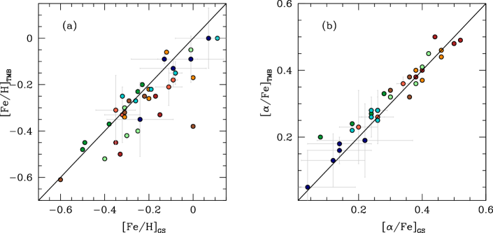
Figure 3: We compare metallicities ([Fe/H]; a) and $\alpha$ abundances ([$\alpha$/Fe] as measured by the Mgb index; b) derived using the prescriptions of Graves & Schiavon (2008) and Thomas et al. (2003) respectively. We show observations for all galaxies at radii out to $2.5R_{e}$. Each galaxy is represented by a different color. The agreement between the two models is decent, with $\langle$[Fe/H]${}_{\rm GS}-$[Fe/H]${}_{\rm TMB}\rangle=-0.06\pm 0.1$, and $\langle$[$\alpha$/Fe]${}_{\rm GS}-$[$\alpha$/Fe]${}_{\rm TMB}\rangle=-0.03\pm 0.08$. To reduce crowding, we include error bars for only two galaxies in the sample.

4.2.1 Uncertainties

Potential contributors to our error budget include random noise, emission line removal, and sky subtraction. We can build the former two into Monte Carlo simulations of our measurement process. For each galaxy, in each radial bin, we start with the best-fit model from GANDALF and create 100 realizations, using the error spectrum generated by Vaccine. We rerun GANDALF and lick_ew on each artificial spectrum and take the error bar as defined by the values encompassing 68% of the mock measurements. Note that the model contains both emission and absorption lines, and thus we should include the uncertainties due to emission line removal naturally in our error budget.

Sky subtraction is a potentially significant source of uncertainty since we are working factors of a few below the level of the sky. In order to quantify how much sky variability effects our final science results we take a heuristic approach. We explore two different scenarios. The first quantifies how changes in the night sky between our two sky nods impacts our final measured EW values. The second test quantifies the effect of an overall over- or under-subtraction of the night sky. In both cases we allow the weighting given to each sky nod to vary, then carry through all the resulting variations in the subtracted science frames. A comparison of the final measured EW values allows for a very direct measure of how well we are handling sky subtraction. We give the details of both scenarios here.

To quantify how changes in the night sky between our two sky nods influence our final measured EW values we explore a range of weighting in the sky nods used for subtraction. For example, if the sky did not vary over the $\sim 45$ minutes between our two sky nods, an equal weighting of 2.0 given to each sky nod would be appropriate. This equates to an equal amount of total exposure time for each sky nod (e.g., 5 min $\times 2.0$ + 5 min $\times 2.0$ = 20 min). However, the sky may evolve on timescales shorter than this. To quantify the effect of an evolving sky on our final science results we ran several different sets of sky nod weightings through our reduction routines and compared the final EW values for all indices. We average deviations over radial bins from $1.5-3R_{e}$. The sky weightings we explored varied by $\pm 20\%$ from 2.0, yet always with a total weighting of 4.0 (e.g. 1.8 for sky nod 1 and 2.2 for sky nod 2). We then make direct comparisons of the EW values ($\delta$EW = EW${}_{\rm orig}-$EW_new) for all of the lines. As the observing conditions were predominantly stable for all our nights, we ran these tests on a single galaxy (NGC 677) and believe it to be representative. The largest $\delta$EW value measured was $0.080\pm 0.098\,$Å (for H$\beta$) when comparing a 2.2 - 1.8 to a 1.8 - 2.2 weighting. The $\delta$EW for each line for the case above were as follows: Mgb = $0.02\pm 0.02\,$Å; H$\beta$ = $0.080\pm 0.1\,$Å; Fe 5270 = $-0.007\pm 0.02\,$Å. From an analysis of the variability of the sky spectra over several nights (Figure 15 in Murphy et al., 2011) the case of 20% variability is extreme. The one exception occurred with IC 1152, which saw a rising moon for some of the exposures. In this case we explored a wide range of sky weights and found a weighting of 2.4 - 1.6 to be optimal.

The second scenario we explore is aimed at understanding what systematic effect over- or under-subtraction of the sky has on our EW values. To test this we conducted a similar set of tests, yet allowed the final weighting of 4.0 to vary. We ran tests exploring both a 5% and 10% over and under subtraction, relative to equal exposure time. We then made the same comparison in $\delta$EW as described above. In the case of a $\pm 5\%$ systematic error in subtraction, we find $\delta$Mg$b$ of $-0.09\pm 0.04\,$Å, $\delta$H$\beta$ of $0.05\pm 0.09\,$Å, and $\delta$¡Fe¿ of $-0.05\pm 0.02\,$Å. The worst deviations in individual bins are at the $0.15\,$Å level in Mg$b$ and H$\beta$ for the 5% oversubtraction case. It is interesting to note that there are not strong systematic effects. Instead we see the indices bounce around at the $0.1-0.15\,$Å level for this level of sky subtraction error. When we get to $10\%$ over-subtraction, the errors are $\delta$Mg$b$ of $-0.2\pm 0.08\,$Å, $\delta$H$\beta$ of $0.01\pm 0.04\,$Å, and $\delta$¡Fe¿ of $-0.04\pm 0.08\,$Å. The worst deviations in individual bins are at the $0.2\,$Å level in Mg$b$ and H$\beta$ for 10% oversubtraction. Larger fractional errors in sky level would lead to obvious residuals in our outer fibers that we do not see. As all of the $\delta$EW values calculated from both tests described here are within our typical uncertainties, and the scenarios we tested were extreme cases, we conclude that our results are robust against sky variations on the scale of $\sim 45$ minutes seen in our data set.

As an additional sanity check of our sky subtraction, we calculate the EW of the Ca H+K $\lambda\lambda 3934,3968$ lines. These features have very high EW, but also are virtually insensitive to changes in stellar populations (at the $\sim 10\%$ level; Brodie & Hanes (1986)). Thus, we expect the line depths to be constant with radius. Because these features are quite blue, they provide a rather stringent test of our fidelity in the sense that the blue spectral shape is most sensitive to errors in sky subtraction. We find that these lines do not vary by more than $10\%$ out to $2.5R_{e}$ for most systems (Figure 2b). As a result, we view our results out to $2.5R_{e}$ as reliable. While we show the point at $2.5-3R_{e}$ in the figures, we will not use that point in our fitting.

4.3 Stellar population modeling

We now convert the observed EWs into ages, metallicities, and abundance ratios using SSP models. Since all indices are blends of multiple elements and all depend on age, metallicity, and abundance ratio to some degree (e.g., Worthey et al., 1994), modeling is required to invert the observed EWs and infer stellar population properties. We compare two different modeling techniques. We first use the methodology outlined in Thomas et al. (2003, 2005). Since the EWs of Mg$b$ and $\langle{\rm Fe}\rangle$ change with both [Fe/H] and [Mg/Fe], these authors construct linear combinations of the two indices. The index [MgFe’]$=\sqrt{(}\rm{Mg{\it b}[0.72\,Fe5270+0.28\,Fe5335]})$ is independent of [Mg/Fe] and tracks [Fe/H], while the index Mgb/$\langle{\rm Fe}\rangle$ depends only on [Mg/Fe]. The pair of derived indices is then inverted to infer metal content and abundance ratios.

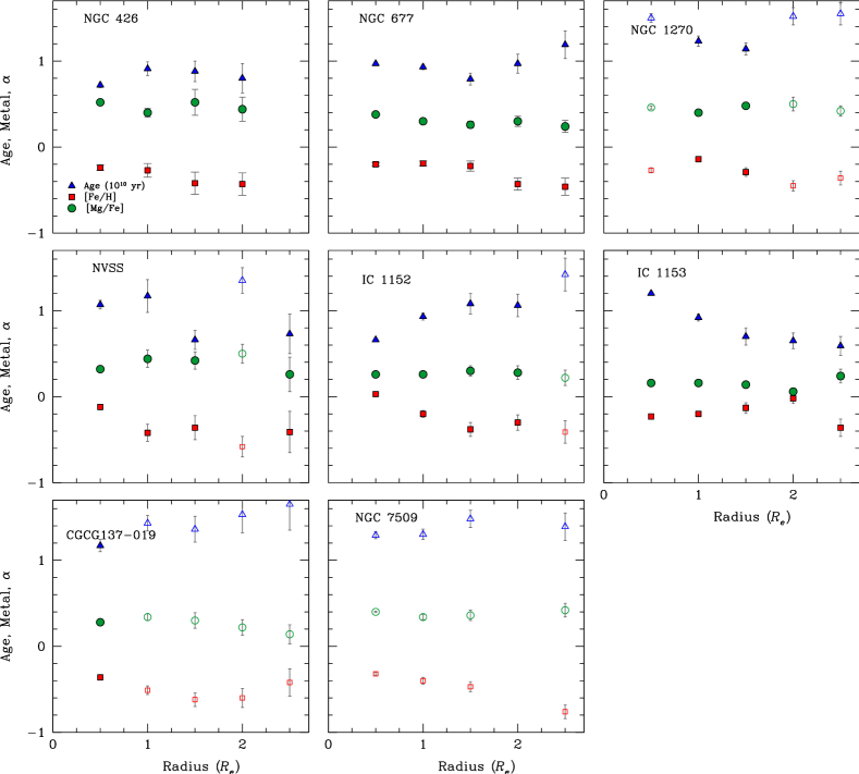
Figure 4: Radial profiles of Age ($10^{10}$ yr; blue triangles), [Fe/H] (red squares), and [Mg/Fe] (green circles) for each galaxy. Radius is measured in units of $R_{e}$. Open symbols are the adjusted values using H$\beta$+$0.2\,$Å, and the two gaps are cases that still fell off of the grid. As above, error bars are derived from Monte Carlo simulations.

We also use the code EZ_Ages by Graves & Schiavon (2008, see also Schiavon 2007). Here, the age, metallicity, and alpha abundance ratios are fit iteratively using the full suite of Lick indices. EZ_Ages solves for the best-fit parameters by taking pairs of measured quantities (e.g., H$\beta$ EW and $\langle{\rm Fe}\rangle$) and then locating the measurements in a grid of model values spanning the full range of age and (in this case) [Fe/H] abundance of the models. The model has a hierarchy of measurement pairs that it considers, first pinning down age and [Fe/H], then looking at [Mg/Fe] and so on. The code then iterates to improve the best fit values. Many more elemental abundances can be fitted by EZ_Ages, thus enabling study of the independent variability of [N/Fe], [C/Fe], etc. There is evidence that individual $\alpha$ elemental ratios vary independently in individual Milky Way stars (e.g., Fulbright et al., 2007) and possibly in galaxies as well (e.g., Kelson et al., 2006; Schiavon, 2007). We do not have adequate S/N in the blue indices to derive other elemental abundances (e.g., Yan, 2011), so we just assume that [Mg/Fe] tracks [$\alpha$/Fe].

The difference between model parameters from EZ_Ages from the observed data and when the H$\beta$ index is boosted by $0.2\,$Å. When H$\beta$ is artificially increased, the ages (blue solid histogram) are lower by $31\pm 5$%, [Fe/H] (red dashed histogram) increases by $0.09\pm 0.01$ dex and [Mg/Fe] (green long-dashed histogram) increases by $0.02\pm 0.01$. When the H$\beta$ EW is too low and falls off of the grid, these corrections are used to put the model parameters based on H$\beta$+$0.2\,$Å on the same scale.

For the remainder of the paper we will use [$\alpha$/Fe] to refer to the $\alpha$-abundance ratios collectively, bearing in mind that we have directly measured [Mg/Fe].

The Thomas et al. (TMB) approach and the Graves & Schiavon (GS) model have somewhat different philosophies, but are inherently similar. Both are based on the inversion of single-burst model grids. Both adjust their primary models for variable $\alpha$-abundance ratios at a range of metallicities. TMB use solar isochrones (Cassisi et al., 1997; Bono et al., 1997) but then modify the indices using the response functions of Tripicco & Bell (1995). GS use solar isochrones from Girardi et al. (2000) and $\alpha$-enhanced isochrones from Salasnich et al. (2000), with the response functions of Korn et al. (2005). TMB invert a small number of high S/N indices, while GS rely on all measured indices in an iterative fashion. In principle we can test some of the systematics of the modeling by comparing our results from the two different approaches.

Finally, note that Graves & Schiavon (2008) parametrize their models in terms of [Fe/H] rather than total metallicity [Z/H], so that they report direct observables. As described in Schiavon (2007, and references therein), we are not able to measure [O/H] directly, and thus cannot truly constrain [$Z$/H]. To compare the two models, we will use the standard conversion (Tantalo et al., 1998; Thomas et al., 2003):

$${\rm[Fe/H]=[Z/H]-0.94[\alpha/Fe]}$$ (1)

In Figure 3 we compare [Fe/H] from Thomas et al. ([Fe/H]_TMB) with that from Graves & Schiavon ([Fe/H]_GS) and likewise for [Mg/Fe], using observations in all radial bins for each galaxy. The agreement is reasonable. Overall, we see a scatter of $\langle$[Fe/H]_GS-[Fe/H]${}_{\rm TMB}\rangle=-0.06\pm 0.1$ for [Fe/H] and $\langle$[$\alpha$/Fe]_GS-[$\alpha$/Fe]${}_{\rm TMB}\rangle=-0.02\pm 0.08$ for [$\alpha$/Fe]. For the rest of the paper we will focus on the EZ_Ages results from Graves & Schiavon, but trust that our results can be directly compared with many in the literature. Also, we have rerun the EZ_Ages modeling with the solar isochrones, and the derived metallicities and $\alpha$-abundance ratios agree within the measurement errors. The radial dependence of the derived quantities for each galaxy is shown in Figure 4.

4.3.1 Low H$\beta$ Equivalent Widths

As mentioned above, there is very likely real but undetectable levels of H$\beta$ emission that slightly lowers the observed H$\beta$ EWs. At the levels measured by Graves & Faber (2010) in composite SDSS spectra ($\sim 0.2\,$Å), the age errors are $\sim 2$ Gyr in general (Schiavon, 2007). In some cases, we cannot derive reasonable model parameters because the measured H$\beta$ EW is too low to fall onto the SSP grids. Since we do not have the S/N needed to correct our spectra on a case by case basis, we use the following procedure to derive model parameters at the radial bins where the H$\beta$ index fall off the bottom of the grid. Note that these corrections are not strictly correct, since the level of emission must vary with radial distance. However, they are the best that we can do at present.

We recalculate the age, [Fe/H], and [Mg/Fe] for all galaxies with the H$\beta$ EW increased by $0.2\,$Å. We then derive an average difference in each measured property between the two sets of models, as shown in Figure 4.3. The differences in [Mg/Fe] and [Fe/H] are very small and (crucially) show no trend with radius, S/N, or H$\beta$ index. The run with increased H$\beta$ EW returns ages that are $31\pm 5\%$ dex lower, [Fe/H] values that are $0.09\pm 0.01$ dex higher and [$\alpha$/Fe] values that are $0.02\pm 0.01$ dex higher on average than the unadjusted data.

We correct the model parameters derived from the H$\beta$+$0.2\,$Å run to align with the fiducial models using the corrections listed above. At each radial bin where we could not derive model parameters using the fiducial H$\beta$ EWs, we instead utilize the corrected model parameters from the H$\beta$+$0.2\,$Å run. In the following, all such points are indicated with open, rather than filled, symbols. With this correction, we derive SSP properties for all but two radials bins over all of the galaxies. Again, applying the same H$\beta$ correction for all points that fall of the grid is not strictly correct, since there is likely radial dependence in the amount of infill. Therefore, we again emphasize that our main strength is in measuring the radial trends rather than the absolute values of the stellar population parameters. Note that Kelson et al. (2006) take a similar, although perhaps more nuanced, approach by shifting all of their model grids to match the Lick indices of their oldest galaxies.

5 The Ages and Metal Contents of Stellar Halos

The most striking trend in Figure 1 is the clear and steady decline in the Mg$b$ index out to large radii. While the gradients vary from object to object, the qualitative behavior is the same for all systems. In contrast, both the $\langle$Fe$\rangle$ index and the H$\beta$ index are generally consistent with remaining flat over the entire radial range. In Table 3 we show the gradients in H$\beta$, $\langle$Fe$\rangle$, and Mg$b$ measured as $\delta$X $\equiv\delta$ log X$/\delta$ log $R/R_{e}$ for each index “X”.

Correlation between the Mg$b$ index and central stellar velocity dispersion. For direct comparison with the literature, we use the stellar velocity dispersion measured within an effective radius, although the differences in dispersion are small as a function of radius (see §5.1 below). We plot measurements for each galaxy at three radii: the central 0.5$R_{e}$ (small red filled circles), between 1.5 and 2 $R_{e}$ (medium yellow circles), and between 2 and 2.5 $R_{e}$ (large blue circles). The S0 galaxies CGCG137-019 and IC 1153 are indicated with a double circle on the central (red) point. For reference, we show the measurements from Graves et al. (2009) as small dots. Since these are SDSS galaxies at $z\approx 0.1$, the light comes from $\sim R_{e}$. We also show the average relation from Trager et al. (2000) as dashed lines, which show the trend line well within the effective radii of average elliptical galaxies. In terms of Mg$b$ EW, the halos of these elliptical galaxies have a similar chemical makeup as galaxies of much lower mass.

We now ask whether the well-known Mg$b$-$\sigma_{\ast}$ relation (e.g., Bender et al., 1993), is preserved at large radii. In Figure 5 we plot the Mg$b$ index at $0.5R_{e}$, $1.5R_{e}$, and $2.5R_{e}$ as a function of galaxy stellar velocity dispersion measured within the effective radius. This figure visually displays two interesting trends. First of all, the Mg$b$ EWs beyond $2R_{e}$ in these massive elliptical galaxies fall significantly below the central Mg$b$-$\sigma_{\ast}$ relation. Matching the Mg$b$ EWs at $2R_{e}$ with the centers of smaller elliptical galaxies suggests that the halo stars were formed in smaller systems. In §5.2 we find that if these stars were accreted from smaller elliptical galaxies, they would come in $\sim 10:1$ mergers. Of course, the more detailed abundance patterns of the halo stars will give us more clues as to the possible origins of these halo stars.

Secondly, we do see hints of a Mg$b$-$\sigma_{\ast}$ correlation even at large radii, but with much more scatter. There is also an intriguing hint that the slope of the Mg$b$-$\sigma_{\ast}$ relation changes. Unfortunately, the correlation is driven to a large degree by the galaxy NGC 1270, which has the largest $\sigma_{\ast}$ value in our sample. NGC 1270 also happens to be our only cluster galaxy. Since the distribution of merger mass ratios is nearly independent of mass (Fakhouri et al., 2010), we might expect the mass of the typical accreted system to rise with mass, thus preserving an Mg$b$-$\sigma_{\ast}$ relation at large radius. However, we will need a larger sample at the highest velocity dispersions to say for certain whether a Mg$b$-$\sigma_{\ast}$ trend continues in the galaxy outskirts.

The next obvious question is whether the Mg$b$ EW drops primarily because of changes in [Fe/H] or [$\alpha$/Fe]. As outlined in the introduction, all evidence suggests that metallicity decline is the primary cause for the decline in Mg$b$ EW. Since very little data exists at such large radii, however, it is worth investigating the [Fe/H] and [$\alpha$/Fe] measurements directly. Again we emphasize that the absolute values of the derived [Fe/H] and [$\alpha$/Fe] are unreliable, but that the gradients should be robust. Below we present gradients in the derived metallicities and abundance ratios in order to determine what drives the striking decline in Mg$b$ EW.

5.1 Gradients

As described above, we measure the gradients $\delta$Age, $\delta$[Fe/H], and $\delta$[Mg/Fe] as $\delta$X $\equiv\delta$ log X$/\delta$ log $R/R_{e}$. We use adjusted values of age, [Fe/H], and [Mg/Fe] for objects that fell off of the grid due to low H$\beta$ EW. We do a very simple least-squares fit to the measured quantities as a function of logarithmic radii in units of $R_{e}$ (Table 3). Only [Fe/H] shows significant evidence for a significant radial gradient. On average, the [$\alpha$/Fe] ratio declines very gently with radius, but the trend is not significant in individual cases. The age gradients take both positive and negative values, but are rarely significant. Given the uncertainties with H$\beta$ described above, we will focus exclusively on metallicity and abundance ratio gradients here.

We should note that unlike most observations in the literature, our fits are weighted towards the outer parts of the galaxies, and we have less spatial resolution in the galaxy centers. We are thus less susceptible to stellar-population variations in the central regions caused by late-time accretion and/or star formation. Indeed, Baes et al. (2007) find a clear break in the slopes of metallicity gradients at small radii, with the gradients getting shallower at larger radii, as do Coccato et al. (2010) for the brightest cluster galaxy in Coma, NGC 4889. Our mild metallicity gradients are similar to those seen at large radius by these authors, as well as by G. Graves & J. Murphy in preparation in M 87.

In principle, correlations between the stellar population gradients and other properties of the galaxy provide additional clues as to the origin of the gradients. We examine the relation between $\sigma_{\ast}$ and gradients in Figure 5. Our results are consistent with the Spolaor et al. (2010) result that the gradients in elliptical galaxies show a larger scatter at higher $\sigma_{\ast}$. In our small sample, we do not find a correlation between the decline in metallicity and the isophote shape, with the metallicity gradients being substantially shallower than the decline in isophote level with radius. We do not find a correlation between gradients in stellar velocity dispersion and gradients in indices or gradients in metallicity or abundance patterns, but the sample is yet small. Eventually it will be interesting to look for correlations between the local escape velocity and the metallicity gradient as may be seen if the metallicity is set locally by the ability of gas to escape the galaxy (Scott et al., 2009; Weijmans et al., 2009).

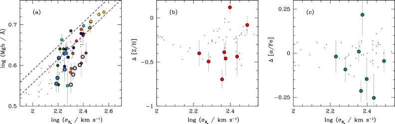
Figure 5: (a): The Mg$b$ index as a function of the stellar velocity dispersion measured at each radial annulus rather than within $R_{e}$. Each galaxy is shown as a different colored circle. The correlation between $\sigma_{\ast}$ and Mg$b$ in individual galaxies as a function of radius is considerably steeper than that seen across galaxy centers. As in Figure 5 above, we show the measurements from Graves et al. (2009) as small dots. Since these are SDSS galaxies at $z\approx 0.1$, the light comes from $\sim R_{e}$. We also show the average relation from Trager et al. (2000), which shows the trend line well within the effective radii of average elliptical galaxies. (b): Gradients in metallicity $\delta$[Z/H]/$\delta$ log ($R/R_{e}$) as compared with the stellar velocity dispersion of the galaxy. Our galaxies are shown as large red circles. We compare with the compilation of Spolaor et al. (2010), and find reasonable agreement in the velocity dispersion range covered by our data. We measure $\sigma_{\ast}$ within $R_{e}$, while Spolaor et al. use $1/8R_{e}$, but the gradients in $\sigma_{\ast}$ over these radii are generally small (e.g., Jorgensen et al., 1995; Cappellari et al., 2006). Also note that Spolaor et al. tabulate gradients out to the effective radii in most cases, while we measure them between $0.5R_{e}$ and $2.5R_{e}$. (c): Same as (b) for gradients in $\delta$[$\alpha$/Fe]/$\delta$ log ($R/R_{e}$) (big green circles). Again note that [Mg/Fe] is assumed to trace [$\alpha$/Fe].

5.2 Where do the Halo Stars Come From?

Figure 5 presents the intriguing possibility that we may uncover the mass scale of accreted satellites by matching the metallicities and abundance ratios of the stellar halos with the centers of smaller elliptical galaxies. In this section we take the measured gradients in Mg$b$ index, [Fe/H], and [Mg/Fe] and attempt to constrain the typical mass of an accreted satellite. As we will show, the abundance patterns in the halo stars do not match the central regions of any local elliptical galaxies, thereby complicating our efforts to find the progenitors of the halo stars. Nevertheless, we can derive an approximate mass ratio from our measured gradients, accepting that present-day galaxies do not form perfect analogs of the accreted satellites.

Using our observed $\sigma_{\ast}$ within $R_{e}$, we assign a central value of abundance ratio and metallicity using the Mg$b$-$\sigma_{\ast}$, [Fe/H]-$\sigma_{\ast}$, and [Mg/Fe]-$\sigma_{\ast}$ relations from Graves et al. (2007). We then use our observed gradients to link the stars at large radii with the $\sigma_{\ast}$ of its most likely progenitor. For instance, we assign an [Fe/H] to each galaxy using the [Fe/H]-$\sigma_{\ast}$ relation from Graves et al. (2007). Then we use our measured gradients to calculate [Fe/H] at $2-2.5R_{e}$. That [Fe/H] value at large radius is matched to the $\sigma_{\ast}$ of an accreted galaxy with the same metallicity using the [Fe/H]-$\sigma_{\ast}$ relation. The derived value of $\sigma_{\ast}$ is translated into a stellar mass $M^{*}$ using the projections of the Fundamental Plane presented by Desroches et al. (2007). The typical mass of accreted galaxies based on each property is shown in Figure 6.2.

Figure 6.2 quantifies the typical mass of accreted satellites. The figure strengthens our conclusion from Figure 5. Based on the Mg$b$ EWs alone, we find that the stars at $>2R_{e}$ were accreted from galaxies $\sim 10$ times less massive than our target galaxies (blue points). However, the figure makes very clear that the metallicities and abundance ratios of our stellar halos cannot be matched with present day elliptical galaxies of any mass. Looked at another way, it says that the [Fe/H] gradients we see in individual halos are steeper than the [Fe/H]-$\sigma_{\ast}$ relation for the population overall, while the [Mg/Fe] gradients are shallower (Figure 5). The Mg$b$-$\sigma_{\ast}$ relation in the galaxy outskirts taken alone suggests that stellar halos are built by $\sim 10:1$ mergers, but the halo stars have lower metallicities and higher $\alpha$-abundance ratios than present-day low-mass ellipticals.

Of course, accreted satellite systems need not be small elliptical galaxies, and may well have started their lives as gas-rich disk galaxies. Thus, it is useful to consider spiral galaxies as well. Since disks also have low surface brightness, there are few studies of abundance patterns in disks based on stellar absorption features (Ganda et al., 2007; Yoachim & Dalcanton, 2008). Furthermore, the interpretation using SSP models is severely complicated by the clear ongoing star formation in these systems (MacArthur et al., 2009). There is general agreement that massive red bulges show similar patterns and scaling relations as elliptical galaxies (e.g., Moorthy & Holtzman, 2006; Robaina et al., 2011). At lower mass, Ganda et al. (2007) find that even the bulge regions of later-type spirals have younger ages, lower metallicities and solar abundance ratios compared to elliptical galaxies.

Due to their protracted star formation histories, present-day late-type spirals do not share the high abundance ratios of the stellar halos studied here. Instead, it may be more productive to consider individual components of present-day galaxies. For instance, thick disks are clearly older than thin disks, and depending on their formation channel may share characteristics of these stellar halos. However, aside from our own galaxy, it remains very difficult to obtain robust stellar abundance patterns in thick disks (Yoachim & Dalcanton, 2008). In Figure 7 we show the abundance ratios at $2-2.5R_{e}$ in our sample as derived using the central relations from Graves et al. and our gradients. We compare with other stellar populations including elliptical and spiral galaxies, and subcomponents of our own galaxy. This figure shows that some of our galaxy halos have similar abundance patterns as the Milky Way thick disk while others are more consistent with low-mass elliptical galaxies. We now address plausible scenarios for how the stellar halos were assembled.

6 Discussion

6.1 Theoretical Expectation

We have established clear gradients in Mg$b$ EW with radius in all of the galaxies in our study. Based on Lick index inversion methods we have argued that in general these gradients are dominated by metallicity with a weak contribution from abundance ratio gradients as well. While the Mg$b$ EWs of the galaxy halos match those of galaxies an order of magnitude less massive, the stars appear to have lower metallicity and higher $\alpha$-abundance ratios than do low-mass ellipticals. We now review the various physical processes that we believe can impact the observed chemistry, in order to determine which scenarios are favored by our observations.

We start with “monolithic” collapse, by which some large fraction of the galaxy is built in a single dissipational burst of star formation (e.g., Eggen et al., 1962). While we believe that we live in a hierarchical Universe in which large galaxies are built up through the merging of smaller parts, the central stellar populations of massive ellipticals clearly imply that their stars were formed rapidly at redshifts $z>2$ (e.g., Thomas et al., 2005, and references therein). A rapid dissipational phase at high redshift is likely an important part of elliptical galaxy formation, followed by late-time dry merging (e.g., Tal et al., 2009; van Dokkum et al., 2010; Newman et al., 2011). There is strong theoretical support for such a “two-phase” picture (e.g., Naab et al., 2009; Oser et al., 2010) and high-redshift progenitors, in which star formation has ceased at early times, are observed (e.g., Kriek et al., 2009).

A large body of work, starting with Larson (1974), has considered the chemical evolution of monolithic collapse models, including a heuristic star-formation law, chemical enrichment, and (typically) galaxy-scale mass loss driven by supernovae. Since these galaxies have deep potential wells, the gas in the center cannot easily be ejected, but instead is enriched by preceding generations of star formation and grows metal-rich. In contrast, in the outer parts of the galaxy, winds can be effective at ejecting metals. Steep gradients in metallicity and $\alpha$ abundance ensue (e.g., Carlberg, 1984; Arimoto & Yoshii, 1987; Kawata & Gibson, 2003; Kobayashi, 2004).

In a modern cosmological context, massive halos that host the progenitors of massive elliptical galaxies are constantly bombarded with smaller halos (e.g., Boylan-Kolchin et al., 2009). Furthermore, we see galaxies merging (Toomre & Toomre, 1972; Schweizer, 1982). Mergers will scramble the orbits of the constituent parts to some degree and wash out metallicity gradients (e.g., White, 1980). The degree of mixing depends on a variety of factors. In a violent relaxation scenario (without dissipation) existing stars may not migrate much, thus preserving the original chemical patterns (van Albada, 1982). In contrast, gas-rich major merging should efficiently supply gas to the center of the remnant, where it will form metal-enriched stars and steepen metallicity gradients (e.g., Mihos & Hernquist, 1996; Cox et al., 2006). Modern simulations that account for cosmological merging and chemical evolution conclude that merger remnants will have shallower metallicity gradients on average, with a much larger scatter than the monolithic collapse case (e.g., Kobayashi, 2004).

6.2 Constraints From Data

Let us briefly review what the observations tell us (see also the introduction for more complete references):

1. There is a strong correlation between Mg$b$ EW and $\sigma_{\ast}$ measured within the effective radius of the galaxy (e.g., Faber, 1973; Dressler et al., 1987; Bender et al., 1993). The majority of this trend is attributed to metallicity, but there is also a trend between $\alpha$-abundance ratio and $\sigma_{\ast}$ (e.g., Worthey et al., 1992; Graves et al., 2009). Much like the mass-metallicity trend observed in star forming galaxies, these trends must arise at some level because of the relative ease of ejecting metals from the shallow potentials of low-mass galaxies (e.g., Dekel & Silk, 1986; Tremonti et al., 2004).

2. In $\sim L*$ elliptical galaxies, the metallicity decreases outwards gently, falling by $\sim 0.1-0.3$ dex per decade in radius. The gradients are too shallow in general to agree with pure monolithic collapse scenarios. No clear trends are seen in $\alpha$-abundance ratio gradients, with increasing, decreasing and flat trends observed (e.g., Kuntschner et al., 2010), again in disagreement with monolithic collapse. In more massive elliptical galaxies, metallicity gradients still dominate, but there is a wider dispersion in the gradient slopes at a given $\sigma_{\ast}$ (Carollo et al., 1993; Spolaor et al., 2010), consistent with what we observe (Figure 5).

3. We add an additional robust spectroscopic point beyond $2R_{e}$. The Mg$b$ EW in the stellar halos match the values seen in local elliptical galaxies that are ten times less massive than our sample galaxies. However, the centers of present-day elliptical galaxies in this mass range have more metals and lower values of [$\alpha$/Fe] than do the stellar halos. Our gradient observations are strongly in contrast with predictions from monolithic collapse scenarios, in which $\alpha$-abundances would decrease outwards (Kobayashi, 2004). The question is whether we can explain the observed stellar properties if the halos were built via minor merging at late times.

At first glance, our observed $\alpha$-abundance ratios are difficult to understand in any scenario. We rule out a pure monolithic-collapse scenario because of the lack of gradient in abundance ratios. Major mergers are not strictly excluded, but seem unable to produce such consistent decreasing metallicity gradients without some tuning. If, in contrast, the outskirts are built up via minor merging at $z<1$ (e.g., Naab et al., 2009), then we would expect the stars to have the same metallicities and abundance patterns as small elliptical galaxies today. Figure 6.2 demonstrates that [$\alpha$/Fe] is too high at a given [Fe/H] to derive from present-day low-mass elliptical galaxies.

The characteristic mass of an accreted satellite at $2.5R_{e}$ as inferred from the Mg$b$ EW (blue circles), [Fe/H] (red squares), and [Mg/Fe] (green triangles). As in Figure 5, S0s are indicated with double circles. To derive the accreted mass, we assume previously derived Mg$b$-$\sigma_{\ast}$, [Fe/H]-$\sigma_{\ast}$, and [Mg/Fe]-$\sigma_{\ast}$ relations (Graves et al., 2007) to assign central values of these quantities to our galaxies. Using our observed gradients, we match the abundance patterns beyond $2R_{e}$ to a present-day elliptical galaxy with the same Mg$b$ EW, [Fe/H], or [Mg/Fe]. We translate the $\sigma_{\ast}$ value to a stellar mass using the Fundamental Plane relations from Desroches et al. (2007). The total galaxy mass derived using the Fundamental Plane is shown with the solid black line. We fit average relations between $\sigma_{\ast}$ and $M_{\rm accreted}$ based on each measurement with a fixed slope to guide the eye only (Mg$b$  dashed blue line; [Fe/H], dot-dashed red line; [Mg/Fe], long-dashed green line). Our indirect technique allows us to circumvent uncertainties in the absolute values of [Fe/H] and [Mg/Fe]. If the stellar halos were constructed from analogs of present-day ellipticals, then the accreted mass derived from each indicator would agree. Instead we find that present-day ellipticals cannot simultaneously match the observed low values of [Fe/H] and high values of [Mg/Fe].

It is useful to draw an analogy with studies of the Milky Way halo. Early suggestions that the halo may be built by the accretion of satellites (Searle & Zinn, 1978) were called into question by the observation that the abundance patterns of stars in the Milky Way halo do not match those of the existing satellites (e.g., Venn et al., 2004, and references therein). However, satellites that are accreted early by the Milky Way will have a truncated star-formation history. Thus, they will have high [$\alpha$/Fe] ratios compared to systems that continue to accrete gas and form stars until the present day (e.g., Robertson et al., 2005; Font et al., 2006). Tissera et al. (2011) track the chemical evolution of eight Milky-Way analogs with hydrodynamical simulations. Most of the mass in each simulated halo is accreted (much of it after a redshift of one) rather than formed in situ. The accreted stars are metal poor and $\alpha$-enhanced, since the stars were predominantly formed at early times in small halos that have truncated star formation histories. We observe the same trend in the halos of the massive early-type galaxies examined here.

Our galaxies are considerably more massive than the Milky Way, and for the most part they do not have disks at the present time. There must be many differences in their merger histories from that of the Milky Way, and the absolute metallicities of the Milky Way halo stars are much lower (Fig. 7). Nevertheless, we suggest that the halos in both cases are built by the accretion of smaller galaxies before these small systems have a chance to self-enrich. Thus, we support a scenario in which massive elliptical galaxies were built up via gas-free minor merging at late times (e.g., Naab et al., 2009). The abundance patterns of the massive halos differ from those seen in $\sim L^{*}$ ellipticals today because the former had their star formation history truncated when they were accreted. In contrast, we know that $\sim L^{*}$ ellipticals had some ongoing star formation at late times (e.g., Babul & Rees, 1992; Thomas et al., 2005; Koleva et al., 2011).

The simulations presented in Oser et al. (2010, see also C. Lackner et al. in preparation) provide strong support for halo build-up via the late accretion of small satellites. They consider galaxies with $M*$ ranging from $5\times 10^{10}-4\times 10^{11}$ $M_{\odot}$, and find that half of the stellar mass was accreted after a redshift of $z\approx 1$. They are able to reproduce the observed size evolution in elliptical galaxies (e.g., van der Wel et al., 2008). Furthermore, they reproduce the observed increase in stellar mass on the red sequence over the last eight billion years (e.g., Faber et al., 2007). Of more direct importance to our story, while accreted late, the majority of the accreted stars were formed at $z\mathrel{\hbox{\hbox to0.0pt{\hbox{\lower 4.0pt\hbox{$\sim$}}\hss}\hbox{\raise 2.0pt\hbox{$>$}}}}3$. These stars were by necessity formed rapidly out of low-metallicity gas. Of course, our sample is still small, but eventually we hope to have a large enough sample to look for differences in elliptical halo abundance patterns as a function of mass.

At a redshift of $z\approx 1$, the progenitors of local $L^{*}$ ellipticals could well have consisted of old, metal-poor, and $\alpha$-enhanced stars. In the schematic picture of Thomas et al. (2005), $\sim L^{*}$ ellipticals are forming the majority of their stars over a few Gyr around $z\lesssim 1$. If roughly half of the stars are formed at $z<1$, with a timescale of $\sim 3$ Gyr, while the original population has [$\alpha$/Fe]=0.2-0.3, the final mass-weighted abundance would be [$\alpha$/Fe]$\approx$0.15, as observed for $L^{*}$ ellipticals today. Thus, those galaxies that are not cannibalized by larger galaxies can easily self-enrich to form the observed populations today. We make a testable prediction of strong evolution in the metallicity and [$\alpha$/Fe] ratios of $\sim L^{*}$ elliptical galaxies from $z\approx 1$ to the present.

In our analysis, we have assumed a constant initial mass function. If instead massive elliptical galaxies have either a top-heavy (van Dokkum, 2008; Davé, 2008) or a bottom-heavy (van Dokkum & Conroy, 2011) initial mass function compared to lower-mass systems, that may change the interpretation of the gradients. We have also ignored the possible variation between different $\alpha$ elements, particularly nitrogen (Schiavon, 2007).

7 Summary

We have used the Mitchell Spectrograph to gather high S/N spectra of eight massive early-type galaxies out to $2.5R_{e}$, in order to study the chemistry of their stellar halos. Looking first at the trends in Lick indices with radius, we find that the EW of Mg$b$ drops, such that the well-known Mg$b$-$\sigma_{\ast}$ relation is not preserved at large radii. Instead the Mg$b$ EWs at large radii are similar to those found in the centers of galaxies that are an order of magnitude less massive.

We show that the well-known metallicity gradients seen within $R_{e}$ continue to the furthest radii probed here. In contrast, [$\alpha$/Fe] does not drop substantially in any object, and certainly never approaches the solar value. Thus, the stars in the outer regions of these elliptical galaxies are metal-poor and $\alpha$-enhanced, much like the stars in the Milky Way halo. We suggest that the outer parts of these galaxies are built up via minor merging with a ratio of $\sim 10:1$, but that the accreted galaxies did not have sufficient time to lower their $\alpha$-abundance ratios to those seen in $\sim L^{*}$ elliptical galaxies today.

We infer the [Fe/H] and [Mg/Fe] values at $2-2.5R_{e}$ using the central relations of (Graves et al., 2007) and our measured gradients (large blue circles). We compare the abundance ratios and metallicites in our stellar halos with Milky Way stars from Venn et al. (2004), including thin disk (small black circles), thick disk (small grey open squares), and halo (small grey stars) stars. For comparison we also show the track of the Graves et al. (2009) composite elliptical galaxies from the SDSS (filled red squares) and the central regions of late-type spiral bulges from Ganda et al. (2007, filled blue triangles). Again, taken as a group, our stellar halos are not well-matched by the integrated properties of galaxy centers today. However, we do see some overlap with Milky Way thick disk stars and low-mass elliptical galaxies.

This paper is only a proof of concept; the Mitchell Spectrograph is ideally suited to study the faint outer parts of galaxies, and there is a considerable amount of follow-up work to be done. First of all, we would like to investigate the kinematics in the outer parts of these galaxies to determine whether there are correlations between angular momentum content and metallicity. We are working on gathering a larger sample, with a full sampling of velocity dispersion, size, and environment, to see whether the radial gradients in (e.g.,) metallicity, correlate with the size of the galaxy at fixed $\sigma_{\ast}$, or the large-scale environmental density. It seems clear that galaxy evolution is accelerated in rich environments (e.g., Thomas et al., 2005; Papovich et al., 2011), leaving subtle imprints in the central stellar populations of galaxies (Zhu et al., 2010). Whether that will leave clear signatures in the gradients remains unknown. Even in our own small sample there are real differences from galaxy to galaxy, and it will be very interesting to see whether the large-scale environment is the cause.

References

- Adams et al. (2012) Adams, J. J., Gebhardt, K., Blanc, G. A., Fabricius, M. H., Hill, G. J., Murphy, J. D., van den Bosch, R. C. E., & van de Ven, G. 2012, ApJ, 745, 92
- Adams et al. (2011) Adams, J. J., et al. 2011, ApJS, 192, 5
- Annibali et al. (2007) Annibali, F., Bressan, A., Rampazzo, R., Zeilinger, W. W., & Danese, L. 2007, A&A, 463, 455
- Arimoto & Yoshii (1987) Arimoto, N., & Yoshii, Y. 1987, A&A, 173, 23
- Babul & Rees (1992) Babul, A., & Rees, M. J. 1992, MNRAS, 255, 346
- Bacon et al. (2001) Bacon, R., et al. 2001, MNRAS, 326, 23
- Baes et al. (2007) Baes, M., Sil’chenko, O. K., Moiseev, A. V., & Manakova, E. A. 2007, A&A, 467, 991
- Barden et al. (1998) Barden, S. C., Sawyer, D. G., & Honeycutt, R. K. 1998, in Society of Photo-Optical Instrumentation Engineers (SPIE) Conference Series, Vol. 3355, Society of Photo-Optical Instrumentation Engineers (SPIE) Conference Series, ed. S. D’Odorico, 892–899
- Bell et al. (2003) Bell, E. F., McIntosh, D. H., Katz, N., & Weinberg, M. D. 2003, ApJS, 149, 289
- Bender et al. (1993) Bender, R., Burstein, D., & Faber, S. M. 1993, ApJ, 411, 153
- Berlind et al. (2006) Berlind, A. A., et al. 2006, ApJS, 167, 1
- Blanc et al. (2009) Blanc, G. A., Heiderman, A., Gebhardt, K., Evans, II, N. J., & Adams, J. 2009, ApJ, 704, 842
- Blanc et al. (2011) Blanc, G. A., et al. 2011, ApJ, 736, 31
- Bono et al. (1997) Bono, G., Caputo, F., Cassisi, S., Castellani, V., & Marconi, M. 1997, ApJ, 489, 822
- Bower et al. (1992) Bower, R. G., Lucey, J. R., & Ellis, R. S. 1992, MNRAS, 254, 601
- Boylan-Kolchin & Ma (2007) Boylan-Kolchin, M., & Ma, C.-P. 2007, MNRAS, 374, 1227
- Boylan-Kolchin et al. (2009) Boylan-Kolchin, M., Springel, V., White, S. D. M., Jenkins, A., & Lemson, G. 2009, MNRAS, 398, 1150
- Brodie & Hanes (1986) Brodie, J. P., & Hanes, D. A. 1986, ApJ, 300, 258
- Brodie et al. (2011) Brodie, J. P., Romanowsky, A. J., Strader, J., & Forbes, D. A. 2011, AJ, 142, 199
- Brough et al. (2007) Brough, S., Proctor, R., Forbes, D. A., Couch, W. J., Collins, C. A., Burke, D. J., & Mann, R. G. 2007, MNRAS, 378, 1507
- Bruzual & Charlot (2003) Bruzual, G., & Charlot, S. 2003, MNRAS, 344, 1000
- Cappellari & Emsellem (2004) Cappellari, M., & Emsellem, E. 2004, PASP, 116, 138
- Cappellari et al. (2006) Cappellari, M., et al. 2006, MNRAS, 366, 1126
- Carlberg (1984) Carlberg, R. G. 1984, ApJ, 286, 416
- Carollo et al. (1993) Carollo, C. M., Danziger, I. J., & Buson, L. 1993, MNRAS, 265, 553
- Cassata et al. (2010) Cassata, P., et al. 2010, ApJ, 714, L79
- Cassisi et al. (1997) Cassisi, S., Castellani, M., & Castellani, V. 1997, A&A, 317, 108
- Cimatti et al. (2008) Cimatti, A., et al. 2008, A&A, 482, 21
- Coccato et al. (2010) Coccato, L., Gerhard, O., & Arnaboldi, M. 2010, MNRAS, 407, L26
- Coelho et al. (2007) Coelho, P., Bruzual, G., Charlot, S., Weiss, A., Barbuy, B., & Ferguson, J. W. 2007, MNRAS, 382, 498
- Conroy & van Dokkum (2011) Conroy, C., & van Dokkum, P. 2011, ApJ, submitted (arXiv:1109.0007)
- Cox et al. (2006) Cox, T. J., Dutta, S. N., Di Matteo, T., Hernquist, L., Hopkins, P. F., Robertson, B., & Springel, V. 2006, ApJ, 650, 791
- Damjanov et al. (2009) Damjanov, I., et al. 2009, ApJ, 695, 101
- Davé (2008) Davé, R. 2008, MNRAS, 385, 147
- de Vaucouleurs (1961) de Vaucouleurs, G. 1961, ApJS, 5, 233
- Dekel & Silk (1986) Dekel, A., & Silk, J. 1986, ApJ, 303, 39
- Desroches et al. (2007) Desroches, L.-B., Quataert, E., Ma, C.-P., & West, A. A. 2007, MNRAS, 377, 402
- Dierckx (1993) Dierckx, P. 1993, Curve and surface fitting with splines, ed. Oxford: Clarendon
- Djorgovski & Davis (1987) Djorgovski, S., & Davis, M. 1987, ApJ, 313, 59
- Dressler et al. (1987) Dressler, A., Lynden-Bell, D., Burstein, D., Davies, R. L., Faber, S. M., Terlevich, R., & Wegner, G. 1987, ApJ, 313, 42
- Dunkley et al. (2009) Dunkley, J., et al. 2009, ApJ, 701, 1804
- Eggen et al. (1962) Eggen, O. J., Lynden-Bell, D., & Sandage, A. R. 1962, ApJ, 136, 748
- Eisenhardt et al. (2007) Eisenhardt, P. R., De Propris, R., Gonzalez, A. H., Stanford, S. A., Wang, M., & Dickinson, M. 2007, ApJS, 169, 225
- Faber (1973) Faber, S. M. 1973, ApJ, 179, 731
- Faber et al. (1977) Faber, S. M., Burstein, D., & Dressler, A. 1977, AJ, 82, 941
- Faber et al. (1985) Faber, S. M., Friel, E. D., Burstein, D., & Gaskell, C. M. 1985, ApJS, 57, 711
- Faber et al. (2007) Faber, S. M., et al. 2007, ApJ, 665, 265
- Fakhouri et al. (2010) Fakhouri, O., Ma, C.-P., & Boylan-Kolchin, M. 2010, MNRAS, 406, 2267
- Finkelstein et al. (2011) Finkelstein, S. L., et al. 2011, ApJ, 729, 140
- Fisher et al. (1995) Fisher, D., Franx, M., & Illingworth, G. 1995, ApJ, 448, 119
- Font et al. (2006) Font, A. S., Johnston, K. V., Bullock, J. S., & Robertson, B. E. 2006, ApJ, 646, 886
- Fulbright et al. (2007) Fulbright, J. P., McWilliam, A., & Rich, R. M. 2007, ApJ, 661, 1152
- Gallagher & Ostriker (1972) Gallagher, III, J. S., & Ostriker, J. P. 1972, AJ, 77, 288
- Gallazzi et al. (2005) Gallazzi, A., Charlot, S., Brinchmann, J., White, S. D. M., & Tremonti, C. A. 2005, MNRAS, 362, 41
- Ganda et al. (2007) Ganda, K., et al. 2007, MNRAS, 380, 506
- Girardi et al. (2000) Girardi, L., Bressan, A., Bertelli, G., & Chiosi, C. 2000, A&AS, 141, 371
- Gonzalez-Perez et al. (2011) Gonzalez-Perez, V., Castander, F. J., & Kauffmann, G. 2011, MNRAS, 411, 1151
- Gorgas et al. (1990) Gorgas, J., Efstathiou, G., & Aragon Salamanca, A. 1990, MNRAS, 245, 217
- Graves & Faber (2010) Graves, G. J., & Faber, S. M. 2010, ApJ, 717, 803
- Graves et al. (2009) Graves, G. J., Faber, S. M., & Schiavon, R. P. 2009, ApJ, 693, 486
- Graves et al. (2007) Graves, G. J., Faber, S. M., Schiavon, R. P., & Yan, R. 2007, ApJ, 671, 243
- Graves & Schiavon (2008) Graves, G. J., & Schiavon, R. P. 2008, ApJS, 177, 446
- Hill et al. (2008a) Hill, G. J., et al. 2008a, in Society of Photo-Optical Instrumentation Engineers (SPIE) Conference Series, Vol. 7014, Society of Photo-Optical Instrumentation Engineers (SPIE) Conference Series
- Hill et al. (2008b) Hill, G. J., et al. 2008b, in Astronomical Society of the Pacific Conference Series, Vol. 399, Panoramic Views of Galaxy Formation and Evolution, ed. T. Kodama, T. Yamada, & K. Aoki, 115
- Hopkins et al. (2009) Hopkins, P. F., Bundy, K., Murray, N., Quataert, E., Lauer, T. R., & Ma, C.-P. 2009, MNRAS, 398, 898
- Jorgensen et al. (1995) Jorgensen, I., Franx, M., & Kjaergaard, P. 1995, MNRAS, 276, 1341
- Kawata & Gibson (2003) Kawata, D., & Gibson, B. K. 2003, MNRAS, 340, 908
- Kelson (2003) Kelson, D. D. 2003, PASP, 115, 688
- Kelson et al. (2006) Kelson, D. D., Illingworth, G. D., Franx, M., & van Dokkum, P. G. 2006, ApJ, 653, 159
- Kelson et al. (2002) Kelson, D. D., Zabludoff, A. I., Williams, K. A., Trager, S. C., Mulchaey, J. S., & Bolte, M. 2002, ApJ, 576, 720
- Kobayashi (2004) Kobayashi, C. 2004, MNRAS, 347, 740
- Koleva et al. (2011) Koleva, M., Prugniel, P., de Rijcke, S., & Zeilinger, W. W. 2011, MNRAS, 417, 1643
- Korn et al. (2005) Korn, A. J., Maraston, C., & Thomas, D. 2005, A&A, 438, 685
- Kriek et al. (2009) Kriek, M., van Dokkum, P. G., Franx, M., Illingworth, G. D., & Magee, D. K. 2009, ApJ, 705, L71
- Kuntschner et al. (2010) Kuntschner, H., et al. 2010, MNRAS, 408, 97
- Larson (1974) Larson, R. B. 1974, MNRAS, 169, 229
- MacArthur et al. (2009) MacArthur, L. A., González, J. J., & Courteau, S. 2009, MNRAS, 395, 28
- Maraston & Stromback (2011) Maraston, C., & Stromback, G. 2011, MNRAS, accepted (arXiv: 1109.0543)
- Mehlert et al. (2003) Mehlert, D., Thomas, D., Saglia, R. P., Bender, R., & Wegner, G. 2003, A&A, 407, 423
- Mihos & Hernquist (1996) Mihos, J. C., & Hernquist, L. 1996, ApJ, 464, 641
- Miller & Owen (2001) Miller, N. A., & Owen, F. N. 2001, ApJS, 134, 355
- Moorthy & Holtzman (2006) Moorthy, B. K., & Holtzman, J. A. 2006, MNRAS, 371, 583
- Murphy et al. (2011) Murphy, J. D., Gebhardt, K., & Adams, J. J. 2011, ApJ, 729, 129
- Naab et al. (2009) Naab, T., Johansson, P. H., & Ostriker, J. P. 2009, ApJ, 699, L178
- Naab et al. (2007) Naab, T., Johansson, P. H., Ostriker, J. P., & Efstathiou, G. 2007, ApJ, 658, 710
- Newman et al. (2011) Newman, A. B., Ellis, R. S., Bundy, K., & Treu, T. 2011, ApJ, submitted (arXiv:1110.1637)
- Ogando et al. (2005) Ogando, R. L. C., Maia, M. A. G., Chiappini, C., Pellegrini, P. S., Schiavon, R. P., & da Costa, L. N. 2005, ApJ, 632, L61
- Oser et al. (2010) Oser, L., Ostriker, J. P., Naab, T., Johansson, P. H., & Burkert, A. 2010, ApJ, 725, 2312
- Papovich et al. (2011) Papovich, C., et al. 2011, ApJ, submitted (arXiv:1110.3794)
- Rawle et al. (2008) Rawle, T. D., Smith, R. J., Lucey, J. R., & Swinbank, A. M. 2008, MNRAS, 389, 1891
- Robaina et al. (2011) Robaina, A. R., Hoyle, B., Gallazzi, A., Jimenez, R., van der Wel, A., & Verde, L. 2011, ArXiv e-prints
- Robertson et al. (2005) Robertson, B., Bullock, J. S., Font, A. S., Johnston, K. V., & Hernquist, L. 2005, ApJ, 632, 872
- Rudick et al. (2010) Rudick, C. S., Mihos, J. C., Harding, P., Feldmeier, J. J., Janowiecki, S., & Morrison, H. L. 2010, ApJ, 720, 569
- Salasnich et al. (2000) Salasnich, B., Girardi, L., Weiss, A., & Chiosi, C. 2000, A&A, 361, 1023
- Sánchez-Blázquez et al. (2007) Sánchez-Blázquez, P., Forbes, D. A., Strader, J., Brodie, J., & Proctor, R. 2007, MNRAS, 377, 759
- Saracco et al. (2010) Saracco, P., Longhetti, M., & Gargiulo, A. 2010, MNRAS, 408, L21
- Sarzi et al. (2006) Sarzi, M., et al. 2006, MNRAS, 366, 1151
- Sarzi et al. (2010) —. 2010, MNRAS, 402, 2187
- Schiavon (2007) Schiavon, R. P. 2007, ApJS, 171, 146
- Schweizer (1982) Schweizer, F. 1982, ApJ, 252, 455
- Scott et al. (2009) Scott, N., et al. 2009, MNRAS, 398, 1835
- Searle & Zinn (1978) Searle, L., & Zinn, R. 1978, ApJ, 225, 357
- Spinrad (1972) Spinrad, H. 1972, ApJ, 177, 285
- Spinrad & Taylor (1971) Spinrad, H., & Taylor, B. J. 1971, ApJS, 22, 445
- Spolaor et al. (2010) Spolaor, M., Kobayashi, C., Forbes, D. A., Couch, W. J., & Hau, G. K. T. 2010, MNRAS, 408, 272
- Strateva et al. (2001) Strateva, I., et al. 2001, AJ, 122, 1861
- Strom & Strom (1978) Strom, K. M., & Strom, S. E. 1978, AJ, 83, 73
- Strom et al. (1976) Strom, S. E., Strom, K. M., Goad, J. W., Vrba, F. J., & Rice, W. 1976, ApJ, 204, 684
- Suh et al. (2010) Suh, H., Jeong, H., Oh, K., Yi, S. K., Ferreras, I., & Schawinski, K. 2010, ApJS, 187, 374
- Tal et al. (2009) Tal, T., van Dokkum, P. G., Nelan, J., & Bezanson, R. 2009, AJ, 138, 1417
- Tantalo et al. (1998) Tantalo, R., Chiosi, C., & Bressan, A. 1998, A&A, 333, 419
- Terlevich et al. (1981) Terlevich, R., Davies, R. L., Faber, S. M., & Burstein, D. 1981, MNRAS, 196, 381
- Thomas et al. (2003) Thomas, D., Maraston, C., & Bender, R. 2003, MNRAS, 339, 897
- Thomas et al. (2005) Thomas, D., Maraston, C., Bender, R., & Mendes de Oliveira, C. 2005, ApJ, 621, 673
- Tifft (1969) Tifft, W. G. 1969, AJ, 74, 354
- Tissera et al. (2011) Tissera, P. B., White, S. D. M., & Scannapieco, C. 2011, MNRAS, accepted (arXiv:1110.5864)
- Toomre & Toomre (1972) Toomre, A., & Toomre, J. 1972, ApJ, 178, 623
- Tortora et al. (2010) Tortora, C., Napolitano, N. R., Cardone, V. F., Capaccioli, M., Jetzer, P., & Molinaro, R. 2010, MNRAS, 407, 144
- Trager et al. (2000) Trager, S. C., Faber, S. M., Worthey, G., & González, J. J. 2000, AJ, 119, 1645
- Tremonti et al. (2004) Tremonti, C. A., et al. 2004, ApJ, 613, 898
- Tripicco & Bell (1995) Tripicco, M. J., & Bell, R. A. 1995, AJ, 110, 3035
- Trujillo et al. (2006) Trujillo, I., et al. 2006, MNRAS, 373, L36
- van Albada (1982) van Albada, T. S. 1982, MNRAS, 201, 939
- van der Wel et al. (2008) van der Wel, A., Holden, B. P., Zirm, A. W., Franx, M., Rettura, A., Illingworth, G. D., & Ford, H. C. 2008, ApJ, 688, 48
- van Dokkum (2008) van Dokkum, P. G. 2008, ApJ, 674, 29
- van Dokkum & Conroy (2011) van Dokkum, P. G., & Conroy, C. 2011, ApJ, 735, L13
- van Dokkum et al. (2008) van Dokkum, P. G., et al. 2008, ApJ, 677, L5
- van Dokkum et al. (2010) —. 2010, ApJ, 709, 1018
- Vazdekis et al. (2010) Vazdekis, A., Sánchez-Blázquez, P., Falcón-Barroso, J., Cenarro, A. J., Beasley, M. A., Cardiel, N., Gorgas, J., & Peletier, R. F. 2010, MNRAS, 404, 1639
- Venn et al. (2004) Venn, K. A., Irwin, M., Shetrone, M. D., Tout, C. A., Hill, V., & Tolstoy, E. 2004, AJ, 128, 1177
- Weijmans et al. (2009) Weijmans, A.-M., et al. 2009, MNRAS, 398, 561
- White et al. (1999) White, R. A., Bliton, M., Bhavsar, S. P., Bornmann, P., Burns, J. O., Ledlow, M. J., & Loken, C. 1999, AJ, 118, 2014
- White (1980) White, S. D. M. 1980, MNRAS, 191, 1P
- Wirth & Shaw (1983) Wirth, A., & Shaw, R. 1983, AJ, 88, 171
- Worthey (1994) Worthey, G. 1994, ApJS, 95, 107
- Worthey et al. (1992) Worthey, G., Faber, S. M., & Gonzalez, J. J. 1992, ApJ, 398, 69
- Worthey et al. (1994) Worthey, G., Faber, S. M., Gonzalez, J. J., & Burstein, D. 1994, ApJS, 94, 687
- Yan (2011) Yan, R. 2011, AJ, 142, 153
- Yan & Blanton (2011) Yan, R., & Blanton, M. R. 2011, ApJ, submitted (arXiv:1109.1280)
- Yoachim & Dalcanton (2008) Yoachim, P., & Dalcanton, J. J. 2008, ApJ, 683, 707
- Yoachim et al. (2010) Yoachim, P., Roškar, R., & Debattista, V. P. 2010, ApJ, 716, L4
- York et al. (2000) York, D. G., et al. 2000, AJ, 120, 1579
- Zhu et al. (2010) Zhu, G., Blanton, M. R., & Moustakas, J. 2010, ApJ, 722, 491
- Zibetti et al. (2005) Zibetti, S., White, S. D. M., Schneider, D. P., & Brinkmann, J. 2005, MNRAS, 358, 949