An attractor for the dynamical state of the intracluster medium

Abstract

Galaxy clusters provide us with important information about the cosmology of our universe. Observations of the X-ray radiation or of the SZ effect allow us to measure the density and temperature of the hot intergalactic medium between the galaxies in a cluster, which then allow us to calculate the total mass of the galaxy cluster. However, no simple connection between the density and the temperature profiles has been identified. Here we use controlled high-resolution numerical simulations to identify a relation between the density and temperature of the gas in equilibrated galaxy clusters. We demonstrate that the temperature-density relation is a real attractor, by showing that a wide range of equilibrated structures all move towards the attractor when perturbed and subsequently allowed to relax. For structures which have undergone sufficient perturbations for this connection to hold, one can therefore extract the mass profile directly from the X-ray intensity profile.

1 Introduction

Galaxy clusters are the largest known gravitationally bound structures in the universe. Consisting almost entirely of dark matter and intracluster gas, they have proved to be very useful objects of study in cosmology. Cluster observations have imposed constraints on the parameters of the $\Lambda$CDM model (Allen et al., 2011; Vikhlinin et al., 2009), and gravitational lensing reveals the galaxies of the distant universe behind the clusters (Kneib et al., 2004). Observations of the gas in galaxy clusters have enabled us to quantify the density profile of dark matter (Buote & Lewis, 2004; Pointecouteau et al., 2005; Host & Hansen, 2011). However, both X-ray and SZ intensity observations suffer from the complication that whereas it is easy to observe the intensity, which is a product of density and temperature, then it is much more complicated to observe the temperature and density separately (Sarazin, 1986). Alternatively, if a simple relation between the density and temperature would exist, one could extract the total mass profile directly from the easily observable X-ray or SZ intensities.

Analytically one might try to search for such a relation by turning to the equation of hydrostatic equilibrium (Cavaliere & Fusco-Femiano, 1976). This equation relates the total mass of a cluster $M_{tot}$ to the gas density $\rho_{g}$ and temperature $T_{g}$ of the intracluster gas. It is given by

$$M_{tot}(r)=-r\frac{k_{B}T_{g}(r)}{\mu m_{u}G}\left(\gamma_{g}(r)+\tau_{g}(r)\right),$$ (1)

where $k_{B}$ is the Boltzmann constant, $\mu$ is the mean molecular mass, $m_{u}$ is the atomic mass unit, $G$ is the gravitational constant and we define $\gamma_{g}=\textrm{d}\ln(\rho_{g})/\textrm{d}\ln(r)$ and $\tau_{g}=\textrm{d}\ln(T_{g})/\textrm{d}\ln(r)$. Unfortunately, for a given $M_{tot}$ we can choose essentially any random $\rho_{g}(r)$ and still make the equation hold by finding a suitable $T_{g}(r)$.

In this Letter we study the evolution of galaxy clusters using hydrodynamical simulations. We find that a wide range of initially equilibrated structures, when dynamically perturbed in order to mimic real perturbations happening during structure formation, all move towards a particular curve in the 2-dimensional phase space spanned by the logarithmic derivatives of the density and temperature of the gas.

2 Initial Conditions

The dimensions of our structures are chosen to resemble those of a large galaxy cluster such as the Perseus Cluster. Each cluster has a scale radius of $r_{0}=100$kpc and a total mass of $10^{15}$M_⊙ of which 10% is gas and 90% is dark matter. They are described by 1 million particles of which 10% represent the gas and 90% represent the dark matter. The mass of the gas and the dark matter particles are thus the same, namely $10^{9}$M_⊙.

To obtain a wide range of initial conditions, we create 20 different structures that vary in both gas and dark matter density profiles as well as dark matter velocity distributions. We use double-power laws to describe the density profiles of the dark matter and the gas.

$$\rho(r)=\rho_{0}\frac{1}{\left(\frac{r}{r_{0}}\right)^{\alpha}}\frac{1}{\left(1+\frac{r}{r_{0}}\right)^{\delta-\alpha}}$$ (2)

Here $\alpha$ and $\delta$ correspond to the inner and outer logarithmic slopes of the density profile respectively. The logarithmic slopes of the dark matter density profiles are chosen in the range $-2\leq\gamma_{dm}\leq 0$ in the inner region and $-6\leq\gamma_{dm}\leq-3.5$ in the outer region. For a given dark matter density profile we use the Eddington method to create isotropic dark matter velocity distributions with $\beta=0$, or the Osipkov-Merrit method to create anisotropic dark matter velocity distributions with $\beta(r)=1/(1+(r_{a}/r)^{2})$, where $r_{a}=r_{0}$ or $r_{a}=2r_{0}$ (Binney & Tremaine, 2008). The logarithmic slopes of the gas density profiles are chosen in the range $-1.5\leq\gamma_{g}\leq 0$ in the inner region and $-5\leq\gamma_{g}\leq-3.5$ in the outer region. For a specific combination of gas and dark matter density profiles we use the equation of hydrostatic equilibrium to find the corresponding gas temperature profiles. Note that $\gamma_{g}$ and $\tau_{g}$ are independent variables. It is therefore, in principle, possible to populate much of the space spanned by $\gamma_{g}$ and $\tau_{g}$.

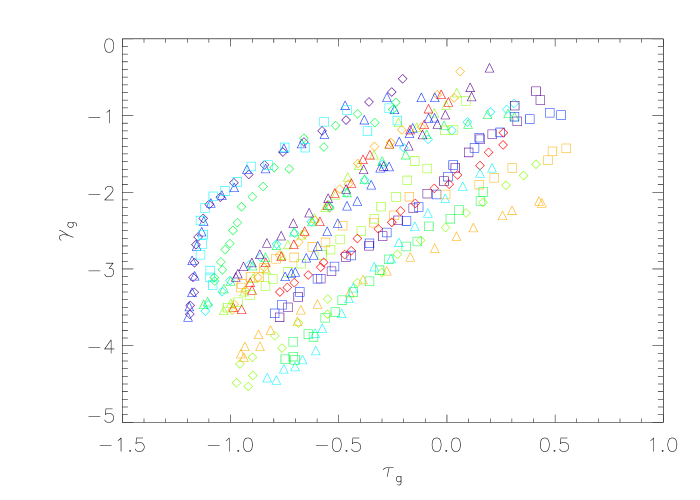
Figure 1: The initial conditions in the $\gamma_{g}=\textrm{d}\ln(\rho_{g})/\textrm{d}\ln(r)$ and $\tau_{g}=\textrm{d}\ln(T_{g})/\textrm{d}\ln(r)$ space. The variations in gas and dark matter density profiles as well as dark matter velocity distributions allow the structures to span a large portion of the $\tau_{g}$-$\gamma_{g}$ space. All the structures of this figure are stable on a timescale of 2 dynamical times when evolved in a hydrodynamical simulation.

All of these initial conditions are presented in Figure 1. To ensure stability these structures have all been evolved for 2 dynamical times, where the dynamical time $t_{dyn}$ = 1.47Gyr has been computed at $R=10r_{0}$. In all figures we only show the region between 3 times the gravitational softening and 10 times the scale radius. The values for $\tau_{g}$ and $\gamma_{g}$ are the average of particles in logarithmically spaced radial bins. We emphasise that our initial conditions both include cool-core clusters with a central $\tau_{g}>0$, as well as non-cool core clusters with a central $\tau_{g}<0$. All these structures are stable on a timescale of 2 dynamical times.

3 Numerical Code

We use the parallel TreeSPH code GADGET-2 to evolve the structures (Springel, 2005). GADGET-2 simulates fluid flows by means of smoothed particle hydrodynamics and computes gravitational forces with a hierarchical tree algorithm. The time integration is based on a quasi-symplectic scheme, where long-range and short-range forces can be integrated with different time steps. Radiative cooling is implemented for a primordial mixture of hydrogen and helium following Katz et al. (1996).

The SPH properties are smoothed over the standard GADGET-2 kernel using $50\pm 1$ SPH particles, while the gravitational forces are adjusted by the gravitational spline kernel using a softening length of 6.0kpc. To protect against too large time steps for particles with very small accelerations, we require that the maximum time step is two percent of the dynamical time of the system. We use an artificial viscosity parameter of $\alpha_{visc}=0.8$ and a courant factor of $\alpha_{cour}=0.1$.

For modelling star formation and the associated heating by supernovae (SN) we follow the sub-resolution multiphase ISM model developed by Springel & Hernquist (2003). In this model, a thermal instability is assumed to operate above a critical density threshold $\rho_{th}$, producing a two-phase medium which consists of cold clouds embedded in a tenuous gas at pressure equilibrium. Stars are formed from the cold clouds on a timescale chosen to match observations (Kennicutt, 1998) and short-lived stars supply an energy of $10^{51}$ergs to the surrounding gas as SN. We adopt the standard parameters for the multiphase model in order to match the Kennicutt Law as specified in Springel & Hernquist (2003). The star formation timescale is set to $t_{*}^{0}=2.1$Gyr, the cloud evaporation parameter to $A_{0}=1000$ and the SN “temperature” to $T_{\rm SN}=10^{8}{\rm}$K. More information on the GADGET version adopted in this work can be found in Moster et al. (2011). All simulations are carried out in a non-cosmological Newtonian box.

4 Perturbations

The cosmological structures we observe today have a long history of hierarchical structure formation involving gravitational collapse and mergers. Both of these are violent relaxation processes that change the gravitational potential and therefore also the energy of the particles according to

$$\frac{\textrm{d}E}{\textrm{dt}}=\frac{\partial\Phi}{\partial t},$$ (3)

for spherical systems, where $E$ is the energy, $\Phi$ is the gravitational potential and $t$ is the time (Lynden-Bell, 1967; Binney & Tremaine, 2008)

To mimic these processes we will expose all our initially equilibrated structures to controlled perturbations. We will require that these perturbations are both continuous and spherical. One example of such perturbations is to let the value of the gravitational constant $G$ vary in the N-body code (Sparre & Hansen, 2012). The perturbations are spherical since the structures themselves are spherical. They are also continuous since they affect the accelerations and not the velocities of the particles.

Initially, we change the value of $G$ by 10%. Setting the gravitational constant equal to $1.1G$ we run the structures for one dynamical time. This will cause the structures to contract, since a higher value of $G$ results in a deeper potential. We then set the gravitational constant equal to $0.9G$ and run the structures for another dynamical time. This will cause the structures to expand since a lower value of $G$ results in a more shallow potential. All in all we submit each structure to a series of 20 perturbations, alternating between a larger and a smaller value of the gravitational constant as described. We check that no unwanted oscillatory behaviour results. We then proceed with ten perturbations where the value of $G$ is changed by 5%, and then ten perturbations where the value of $G$ is changed by only 1%. Finally, we let the structures run for an additional 10 dynamical times with a normal value of $G$ to make sure they are in equilibrium.

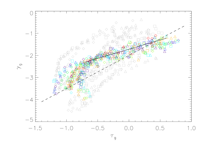
Figure 2: The same phase space as in Figure 1 is now populated by the final equilibrated profiles of the perturbed structures. Note that the initial conditions (light grey symbols) have approached the 1-dimensional line, the attractor, from both sides. Also shown is a line of the form $\rho_{g}/T_{g}^{3/2}\sim r^{-2}$ (dashed), and a linear guide-the-eye line of the form $\gamma_{g}=0.83\tau_{g}-1.72$ in the region $-0.7<\tau_{g}<0.6$ (solid).

5 The Attractor Solution

The results of the perturbations are presented in Figure 2, from which it is clear that all the structures end up along the same curve. It is important to emphasise that we had initial conditions both above and below this attractor solution. The particles in the outer region (small $\tau$) still tend to follow the initial conditions. This is partly because they have not been perturbed as much due to their larger dynamical time.

For the final structures the formed stars dominate the total mass within $r=20$kpc, and they contribute significantly to the collisionless component within $r=100$kpc. To determine how much of an effect the star formation has had on the attractor, we first perform a simulation in which the density threshold for star formation, $\rho_{th}$, is ten times larger than normal. This has the effect of suppressing the star formation. However, the structure still ends up along the attractor suggesting that the star formation itself does not have much of an effect.

We also perform a run of only 20 perturbations of 10%. After that we let the structure relax for 30 dynamical times. Again, the structure does not stray from the attractor at all, showing that it is not affected by the formation of stars even over such a long period of time.

To quantify how much the attractor solution stands out compared to the initial conditions we introduce the structure-to-structure dispersion $\sigma_{S2S}^{2}(\tau_{g})$, which describes the spread among a group of structures as a function of $\tau_{g}$. This value is expected to be significantly larger for the initial conditions than for the perturbed structures, because the different structures make clearly distinct lines in Figure 1. One can define

$$\sigma_{tot}^{2}(\tau_{g})=\sigma_{S2S}^{2}(\tau_{g})+\sigma_{int}^{2}(\tau_{g}),$$ (4)

where $\sigma_{tot}^{2}(\tau_{g})$ is the total spread of data points, and $\sigma_{int}^{2}(\tau_{g})$ is the average internal spread of the individual structures. Perfectly smooth structures with infinitely many particles would thus have $\sigma_{int}^{2}(\tau_{g})\approx 0$. Binning the data points with respect to $\tau_{g}$ we consider a single bin $i$ with $N$ data points. Since the data points are not distributed symmetrically around an average value of $\gamma_{g}$, we define the median value of $\gamma_{g}$ as the one for which 50% of the data points lie to either side. Similarly, counting 15.8% from the left (one standard deviation) we find

$$\sigma_{-}(\tau_{g}^{i})=|\gamma_{g}^{i}(50-15.8\textrm{ percentile})-\gamma_{g}^{i}(50\textrm{ percentile})|,$$ (5)

and counting 15.8% from the right we find

$$\sigma_{+}(\tau_{g}^{i})=|\gamma_{g}^{i}(50+15.8\textrm{ percentile})-\gamma_{g}^{i}(50\textrm{ percentile})|.$$ (6)

We now define

$$\sigma_{tot}^{2}(\tau_{g}^{i})=\left(\frac{\sigma_{-}(\tau_{g}^{i})+\sigma_{+}(\tau_{g}^{i})}{2}\right)^{2}$$ (7)

and its error

$$\delta\sigma_{tot}^{2}(\tau_{g}^{i}) = \frac{1}{2}\left((\sigma_{-}(\tau_{g}^{i})-\sigma_{tot}(\tau_{g}^{i}))^{2}+(\sigma_{+}(\tau_{g}^{i})-\sigma_{tot}(\tau_{g}^{i}))^{2}\right)$$ (8)

$$= {\left(\frac{\sigma_{+}(\tau_{g}^{i})-\sigma_{(}\tau_{g}^{i})-}{2}\right)^{2}.}$$

For a single structure with $M$ radial bins we define

$$\Delta\gamma_{g}^{j}=\gamma_{g}^{j}-\hat{\gamma}_{g}^{j}$$ (9)

as the distance between a point $\gamma_{g}^{j}$ and its interpolated value

$$\hat{\gamma}_{g}^{j}=\gamma_{g}^{j-1}+\frac{\gamma_{g}^{j+1}-\gamma_{g}^{j-1}}{\tau_{g}^{j+1}-\tau_{g}^{j-1}}(\tau_{g}^{j}-\tau_{g}^{j-1}).$$ (10)

Here $j$ refers to a given radial bin. Again, binning in $\tau_{g}$ we define for a single bin $i$ with $K$ data points the value of $\sigma_{int}^{2}(\tau_{g}^{i})$ as the median value of $(\Delta\gamma_{g})^{2}$. For the distribution we again count 15.8% from left and right and take the average to to find the error $\delta\sigma_{int}^{2}(\tau_{g}^{i})$. We do not include any points for which $\gamma_{j}<-3.5$.

The spread between the initial and final structures are presented in Figure 3.

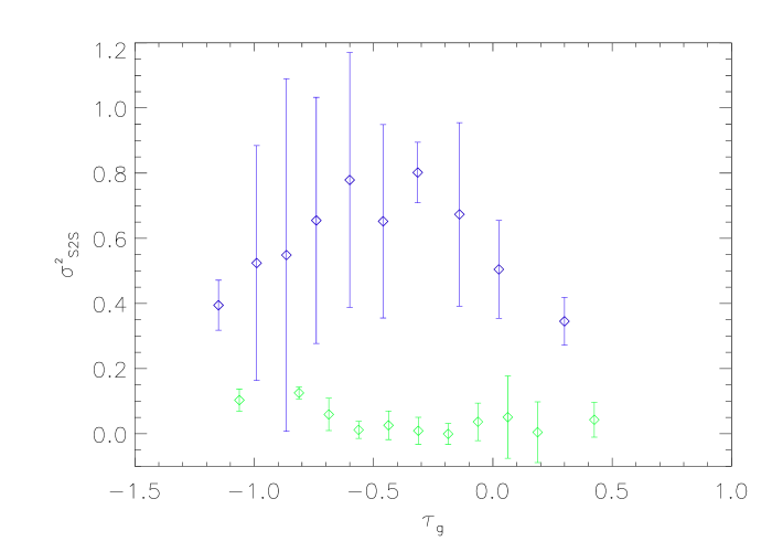
Figure 3: The structure-to-structure dispersion, describing the off-set between a group of different structures. The initial conditions (blue) cover a large fraction of the phase space $(\tau_{g},\gamma_{g})$, whereas the final (green) structures end essentially on top of each other, resulting in a very small $\sigma_{S2S}^{2}$.

Since the initial conditions span a large portion of the $\gamma_{g}-\tau_{g}$ space they consequently have a relatively large $\sigma_{S2S}^{2}$, while the final structures, which generally lie along the same curve, have a distinctly smaller $\sigma_{S2S}^{2}$.

6 Discussion

In Figure 2 we plot a line of the form $\rho_{g}/T_{g}^{3/2}\sim r^{-\alpha}$, corresponding to the entropy following a power-law in radius, where $\alpha$ is an unknown constant. This implies $\gamma_{g}=-\alpha+3/2\,\tau_{g}$. This possibility has been discussed intensively in the literature (see e.g. Morandi & Ettori, 2007; Pratt et al., 2010; Dubois et al., 2011, for references). In the figure we use $\alpha=2$. Our resulting attractor clearly differs from this simple behaviour, both in the inner and the outer region.

We also include a linear guide-the-eye line of the form $\gamma_{g}=0.83\tau_{g}-1.72$. Although this is obvious a simplified approximation it provides an acceptable fit in the range $-0.7<\tau_{g}<0.6$.

We note that our limited resolution does not allow us to resolve the inner region where $\gamma_{g}>-1$. That region is particularly interesting when one is considering cool-core clusters where $\tau_{g}$ may be large and positive. Initially the rapid cooling in our simulations forms a large central stellar condensation, which acts like a (unrealistically large) central blue BCG, a problem which possibly could be reduced by including AGN feedback. Subsequently, our perturbations are likely inducing adiabatic compression shocks, which helps (together with the SN feedback) preventing the structures from undergoing further rapid cooling, in fact, we do not observe any late time cooling catastrophe despite our simulation effectively being longer than a Hubble time. This may also be connected to the fact that the quickly formed central BCG may act like a stabilizing structure which helps preventing rapid over cooling from destabilizing the structure (Li & Bryan, 2011).

This simple connection allows one to write a simplified hydrostatic equilibrium equation, $M_{\rm tot}=f_{1}(T_{g})$, where $f_{1}(T_{g})$ is a known function only of the gas temperature, with no reference to the gas density. Alternatively, if we knew the absolute value of the temperature at one point, then one could write this as $M_{\rm tot}=f_{2}(\rho_{g})$, where $f_{2}(\rho_{g})$ is a known function only of the gas density, or even better, $M_{\rm tot}=f_{3}(I)$, where $f_{3}(I)$ is a known function only of the gas intensity, which is easily observable even at high redshift.

It has long been observed that the characteristic radius for the temperature (at $T_{\rm max}$) roughly corresponds to the scale radius for the gas density (see e.g. Vikhlinin et al., 2006). We now see how this relates to the attractor presented here: The radius corresponding to $\tau_{g}=0$ should have $-2<\gamma_{g}<-1.5$, which is close to the scale radius of the density profile

A connection has previously been suggested between the gas temperature profile and the dark matter dispersion (Hansen & Piffaretti, 2007), which is not only a fair approximation for galaxy clusters (Frederiksen et al., 2009; Host et al., 2009; ZuHone, 2011), but also holds well for the hot gas in galaxies as well as near AGN (Hansen et al., 2011). We find that the corresponding structure-to-structure dispersion for this gas-DM temperature connection is larger, and we therefore conclude that the gas-density connection presented in this paper is likely more fundamental.

When comparing our finding here with the recent discovery of an attractor for dark matter structures, a remarkable suggestion presents itself. The dark matter attractor is a 1-dimensional line in a 3-dimensional space spanned by $\gamma_{dm},\tau_{dm}$ and $\beta_{dm}$, where the first two are the logarithmic derivatives of the dark matter density and radial velocity dispersion ($\sigma_{r}^{2}$, which acts like a temperature per mass), and $\beta_{dm}$ is the velocity anisotropy (Hansen, Juncher & Sparre, 2010). The Jeans equation, which is the dark matter equivalent of the hydrostatic equilibrium, can be written as

$$M_{tot}(r)=-r\frac{\sigma_{r}^{2}}{G}\left(\gamma_{dm}(r)+\tau_{dm}(r)+2\beta_{dm}(r)\right)\,.$$ (11)

We therefore see that the dark matter attractor is between elements in the parenthesis in the Jeans equation, eq. (11), and the gas attractor presented in this paper is between the elements in the parenthesis in the equation for hydrostatic equilibrium, eq. (1). We therefore speculate, that if one will manage to derive the gas attractor we present here, then one may possibly use that understanding to derive the attractor for the dark matter as well.

It is important to emphasize that the attractor for the gas is not just an reaction to the changes in the dark matter as it adjusts to its own attractor. Two of our initial structures start right on the dark matter attractor but not on the gas attractor. When they are perturbed they move to the gas attractor while staying on the dark matter attractor.

In this paper we have only investigated the effect of the particular $G$-perturbation. We note that the resulting dark matter density profiles are different, and the gas attractor is thus not a trivial result of the perturbation driving the dark matter structures towards a universal density profile. It has been shown for the dark matter attractor that a wide range of perturbations all lead to the same attractor (Hansen, Juncher & Sparre, 2010; Sparre & Hansen, 2012; Barber et al., 2012), suggesting that our found gas attractor is likely not a result of the particular perturbation chosen here. In the future we intend to study which effects more realistic perturbations, such as minor or major mergers, will have on the gas attractor. We also note that the simulations presented here both have gas and dark matter, however, when analysing the 3-dimensional dark matter phase space, we find that the dark matter attractor is slightly shifted compared to the cases including only dark matter.

7 Conclusions

Using high-resolution numerical simulations of large galaxy clusters, including radiative cooling, star-formation and feedback, we identify an attractor for the hot gas component. This attractor gives a very simple connection between the temperature and the density of the gas.

We find the attractor to hold for all structures which have been exposed to significant perturbations and subsequently allowed to relax. Since cosmological structures experience perturbations during mergers, we speculate that the central part of galaxy clusters, which are fully equilibrated, may follow the attractor. It will be very interesting in the near future to test this suggestion on real X-ray observations.

References

- Allen et al. (2011) Allen, S. W., Evrard, A. E., & Mantz, A. B. 2011, ARA&A, 49, 409
- Barber et al. (2012) Barber, J. et al. 2012, to appear
- Binney & Tremaine (2008) Binney, J., & Tremaine, S. 2008, Galactic Dynamics: Second Edition. Princeton University Press
- Buote & Lewis (2004) Buote, D. A., & Lewis, A. D. 2004, ApJ, 604, 116
- Cavaliere & Fusco-Femiano (1976) Cavaliere, A., & Fusco-Femiano, R. 1976, A&A, 49, 137
- Dubois et al. (2011) Dubois, Y., Devriendt, J., Teyssier, R., & Slyz, A. 2011, MNRAS, 417, 1853
- Frederiksen et al. (2009) Frederiksen, T. F., Hansen, S. H., Host, O., & Roncadelli, M. 2009, ApJ, 700, 1603
- Hansen & Piffaretti (2007) Hansen, S. H., & Piffaretti, R. 2007, A&A, 476, L37
- Hansen, Juncher & Sparre (2010) Hansen, S. H., Juncher, D., & Sparre, M. 2010, ApJ, 718, L68
- Hansen et al. (2011) Hansen, S. H., Macciò, A. V., Romano-Diaz, E., et al. 2011, ApJ, 734, 62
- Host et al. (2009) Host, O., Hansen, S. H., Piffaretti, R., et al. 2009, ApJ, 690, 358
- Host & Hansen (2011) Host, O., & Hansen, S. H. 2011, ApJ, 736, 52
- Katz et al. (1996) Katz, N., Weinberg, D. H., & Hernquist, L. 1996, ApJS, 105, 19
- Kennicutt (1998) Kennicutt, R. C., Jr. 1998, ApJ, 498, 541
- Kneib et al. (2004) Kneib, J.-P., Ellis, R. S., Santos, M. R., & Richard, J. 2004, ApJ, 607, 697
- Li & Bryan (2011) Li, Y., & Bryan, G. L. 2011
- Lynden-Bell (1967) Lynden-Bell, D. 1967, MNRAS, 136, 101
- Morandi & Ettori (2007) Morandi, A., & Ettori, S. 2007, MNRAS, 380, 1521
- Moster et al. (2011) Moster, B. P., Macciò, A. V., Somerville, R. S., Naab, T., & Cox, T. J. 2011, MNRAS, 415, 3750
- Pointecouteau et al. (2005) Pointecouteau, E., Arnaud, M., & Pratt, G. W. 2005, A&A, 435, 1
- Pratt et al. (2010) Pratt, G. W., Arnaud, M., Piffaretti, R., et al. 2010, A&A, 511, A85
- Sarazin (1986) Sarazin, C. L. 1986, Reviews of Modern Physics, 58, 1
- Sparre & Hansen (2012) Sparre, M., & Hansen, S. H. 2012, to appear
- Springel & Hernquist (2003) Springel, V., & Hernquist, L. 2003, MNRAS, 339, 289
- Springel (2005) Springel, V. 2005, MNRAS, 364, 1105
- Vikhlinin et al. (2006) Vikhlinin, A., Kravtsov, A., Forman, W., et al. 2006, ApJ, 640, 691
- Vikhlinin et al. (2009) Vikhlinin, A., Kravtsov, A. V., Burenin, R. A., et al. 2009, ApJ, 692, 1060
- ZuHone (2011) ZuHone, J. A. 2011, ApJ, 728, 54