Quantitative analyses of empirical fitness landscapes

Abstract

The concept of a fitness landscape is a powerful metaphor that offers insight into various aspects of evolutionary processes and guidance for the study of evolution. Until recently, empirical evidence on the ruggedness of these landscapes was lacking, but since it became feasible to construct all possible genotypes containing combinations of a limited set of mutations, the number of studies has grown to a point where a classification of landscapes becomes possible. The aim of this review is to identify measures of epistasis that allow a meaningful comparison of fitness landscapes and then apply them to the empirical landscapes to discern factors that affect ruggedness. The various measures of epistasis that have been proposed in the literature appear to be equivalent. Our comparison shows that the ruggedness of the empirical landscape is affected by whether the included mutations are beneficial or deleterious and by whether intra- or intergenic epistasis is involved. Finally, the empirical landscapes are compared to landscapes generated with the Rough Mt. Fuji model. Despite the simplicity of this model, it captures the features of the experimental landscapes remarkably well.

1 Introduction

How genotypes map onto phenotypes is one of the central questions in biology. Developmental and systems biologists seek to understand the physical, biochemical and physiological basis of the genotype-phenotype map, while evolutionary biologists study its evolutionary causes and consequences [1, 2, 3]. To predict the evolutionary fate of a genotype it is essential to understand how genotypes map onto fitness – the basic predictor of an organism’s evolutionary success. This has led to the notion of a fitness landscape [4, 5], which is a mapping from the multidimensional genotype space to a real-valued measure of fitness. Graphical renderings often depict the fitness landscape as a surface above a two-dimensional base plane symbolizing the genotype space, but it is clear that such a low-dimensional representation is generally inadequate to provide more than a rather superficial, metaphoric description of the evolutionary process (for an alternative visualization see fig.1). The limitations of the two-dimensional representation have spawned much fundamental criticism of the fitness landscape concept. Here, rather than abandoning the concept altogether, we take the view that ”fitness landscapes…should be studied in less picturesque but more quantitative ways” [6].

Within the fitness landscape metaphor, adaptation is imagined as a hill-climbing process leading the population to a fitness peak, with distinct roles for both natural selection and genetic drift [7, 8]. The structure of the fitness landscape can range from smooth with few accessible peaks to rugged with multiple peaks separated by valleys of low fitness. Whether the landscape is smooth or rugged has important consequences for evolution [9, 10]. For instance, the topography of the fitness landscape affects speciation via reproductive isolation [11, 12], the evolutionary benefits of sex and recombination [13, 14], the evolution of genetic robustness and evolvability [15, 16, 17], and the predictability of evolution [7, 18, 19, 20].

Little is known about the factors that determine the topography of a fitness landscape, beyond the general notion that epistasis is involved. The term epistasis as defined by Fisher [21] includes all deviations from the additive effects of alleles at different loci, and is usually considered for two alleles only. To understand the role of epistasis in shaping the structure of fitness landscapes we need to distinguish between magnitude and sign epistasis [22]. Magnitude epistasis is present when the fitness effect of a mutation at a given locus has a definite sign (beneficial or deleterious) irrespective of the alleles at other loci, while the magnitude depends on the genetic background. Magnitude epistasis does not constrain accessibility of mutational trajectories in an absolute sense and only affects the curvature of a landscape, which can be quantified by a quadratic regression of mean fitness on mutation number. On the other hand, sign epistasis occurs when mutations are beneficial in some genetic backgrounds, but not in others. Hence, the sign (positive or negative) of an allelic effect changes with the presence of an allele at another locus. Sign epistasis causes pathways to become inaccessible by natural selection and thus introduces ruggedness into the landscapes [17, 22]. A special case of sign epistasis, called reciprocal sign epistasis, occurs when the sign of both alleles’ fitness effects changes with a change of alleles at the other locus. Reciprocal sign epistasis is a prerequisite for the occurrence of multiple fitness peaks [23, 24].

A related but distinct classification of epistatic interactions discerns between unidimensional and multidimensional epistasis [2, 12]. In the unidimensional case fitness can be written in terms of a scalar function of the genotype, such as the number of loci carrying a mutation, whereas multidimensional epistasis includes all allelic interactions. Generic fitness landscapes are expected to display both sign epistasis and multidimensional epistasis. Nevertheless, in empirical studies a unidimensional fitness function has often been assumed by averaging over different allelic combinations carrying the same number of mutations. Such an approach can be misleading, because a seemingly additive unidimensional fitness landscape may result from the cancellation of multidimensional epistatic interactions [25].

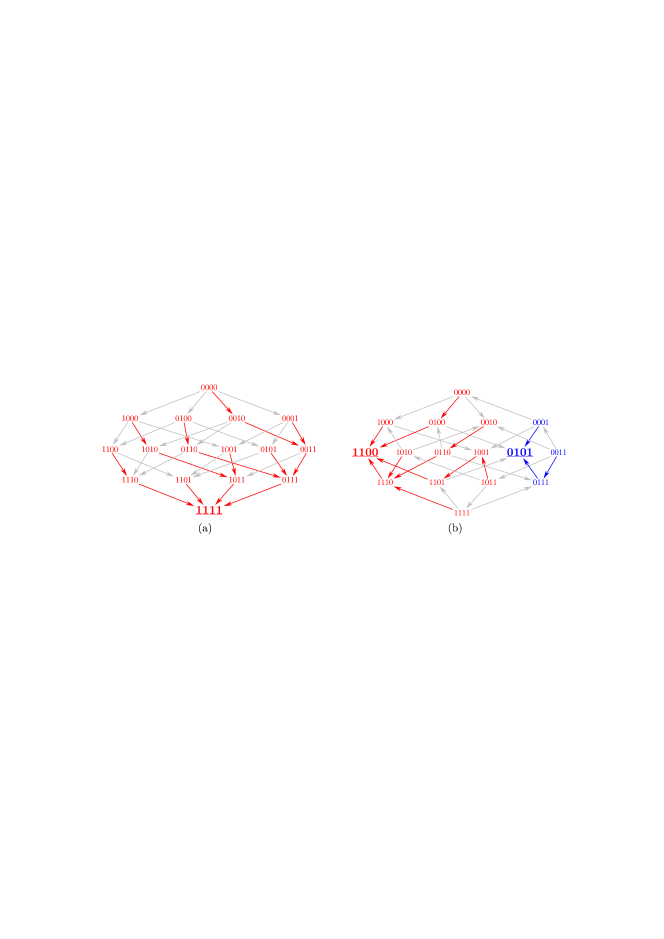
Figure 1: The figure shows two examples of empirical fitness landscapes containing all combinations of mutations at $L=4$ loci. Genotypes are represented by binary sequences, where 0 (1) indicates the absence (presence) of the corresponding mutation. Arrows point in the direction of increasing fitness, and underlined nodes correspond to fitness maxima. Colored arrows point towards the fittest neighbor, forming the basins of attraction of a steepest ascent (“greedy”) adaptive walk. (a) Fitness landscape based on four beneficial mutations in the bacterium Methylbacterium extorquens [26] (landscape A in Tables 1 and 2). (b) Fitness landscape based on four mutations in a malaria drug resistance gene [27]. The fourfold mutant $\{1111\}$ confers maximal drug resistance but does not optimize the growth rate in the absence of the drug, which is the quantity used here as a proxy for fitness (landscape D in Tables 1 and 2).

In theory, with full knowledge of a fitness landscape, one overlooks all possible evolutionary pathways connecting two genotypes, and would be able to determine the likelihood that particular pathways are taken. This would render evolution predictable in a restricted (i.e., a posteriori) sense. However, these predictions are valid for a specific combination of genotype and environment, and also depend on population dynamic parameters such as population size and mutation rate. Another limitation is that one can only study a tiny part of sequence space explicitly, because the number of genotypes grows beyond comprehension with the number of loci considered. Even for a single gene of 1000 base-pairs and when allowing only point mutations, the number of possible genotypes ($4^{1,000}$) is larger than the total number of particles in the universe, as Sewall Wright [5] realized. This scale problem has two immediate implications. First, it emphasizes the fundamentally stochastic nature of evolution, given how little of genotype space has been probed by life since it exists. Second, if we are to use the growing amount of information about the genetic make-up of organisms to understand and ultimately predict evolution, we need to invoke models of fitness landscapes parametrized by empirical observations.

The purpose of this review is to compare the topographies of empirical fitness landscapes that recently have been published. Before doing so, we briefly survey the main models of fitness landscapes in which ruggedness can be tuned, as well as the different approaches to study fitness landscapes empirically. Recent efforts have been directed towards constructing all $2^{L}$ possible genotypes containing combinations of a limited set of $L$ mutations, and measuring their fitness or a proxy thereof [2], see fig.1 for two examples. First, we compare different measures of ruggedness and sign epistasis derived from the available landscapes, and find that these correlate well and thus appear to be equivalent. Second, using these robust measures of ruggedness we can compare the ruggedness of different empirical landscapes despite of methodological differences and the variety of biological systems involved. We find that those landscapes built from mutations that are known to have a combined beneficial effect are less rugged than those built from mutations that are selected without regard to their combined effect, in particular when they are deleterious. Third, we compare the empirical fitness landscapes to a simple statistical one-parameter model, the Rough Mt. Fuji model, which combines a linear fitness trend with uncorrelated random fitness variations. We find that this model captures the features of the empirical landscapes surprisingly well.

2 Fitness landscape models

Until recently empirical information about the structure of fitness landscapes was largely unavailable, and the number of studies is currently still small. Therefore, past studies of fitness landscapes have been mostly restricted to theoretical work. The models proposed in this context are based on very different - and sometimes even contradicting - intuitions. In this section, we give a brief overview of the most popular models. Throughout we represent genotypes by binary strings $\vec{\sigma}=(\sigma_{1},\sigma_{2},...,\sigma_{L})$ of length $L$, where $\sigma_{i}=0$ (1) if the mutation at the $i$-th locus is absent (present), compare to fig.1.

2.1 Kauffman’s $LK$ model

If a given gene $A$, when expressed, produces an essential protein that requires the presence of another protein produced by gene $B$ to function properly, these two genes interact epistatically. When gene $A$ is expressed independently of gene $B$, an organism with a defective mutation in gene $B$ incurs the cost of producing the protein from gene $A$ without experiencing its beneficial effect. The mutation in gene $B$ can thus change the fitness contribution of gene $A$ from beneficial to deleterious, resulting in sign epistasis. The main motivation of the $LK$ model as proposed by Kauffman and Weinberger [28, 29] is to capture such strong, sign-epistatic effects of single mutations in interacting genes on fitness in a statistical sense, without attempting a detailed biochemical description.

The interactions are modeled as evenly spread across the entire genome. The genome is represented as a binary sequence of length $L$ and the interactions take the form of a set of sites called interaction partners $\vec{\nu}_{i}\equiv\{i,\nu_{i,1},\nu_{i,2},\dots,\nu_{i,K}\}$ associated with each site $i$ of the genome. The number $K$ of interaction partners is kept constant. How partner sites are assigned has implications for search strategies for the global optimum on the landscapes [31], but most often the interaction partners are chosen by picking them uniformly and independently at random (making sure that no site appears twice in a given set $\vec{\nu_{i}}$). The fitness of an organism with genome $\vec{\sigma}$ is then the sum of the individual fitness contributions,

$$f(\vec{\sigma})=\sum_{i=1}^{L}f_{i}(\{\sigma_{j}\}_{j\in\nu_{i}}).$$ (1)

The single site contributions $f_{i}$ are independent and identically distributed random variables (i.i.d. RV’s) associated with each of the $2^{K+1}$ possible states of the argument. If a mutation hits part of the sequence that does not appear in the argument of $f_{i}$, i.e. if the mutation does not involve the site $i$ or any of the associated partner sites in $\vec{\nu}_{i}$, the fitness contribution $f_{i}$ remains unchanged, otherwise it is replaced by an independent random number.

For $K=0$, each contribution $f_{i}$ can only take two possible values, corresponding to $\sigma_{i}=0$ or $1$, respectively. Thus each site has one state that is more beneficial than the other and since the fitness of a sequence is the sum over the site contributions, the global optimum is at the state with all sites in their ‘beneficial’ position. The global optimum can be reached from any initial configuration by mutating sites into their beneficial state in a random order, which implies that all mutational pathways are accessible and sign epistasis is absent. Conversely, when $K=L-1$, the entire sequence appears in the argument of each single site contribution. Thus any mutation replaces the sum (1) by a sum over a different set of i.i.d. RV’s, which is equivalent to replacing one i.i.d. RV by another. The number of sites in the partner set, denoted by $K$, thus allows one to tune the strength of epistatic interactions from the non-epistatic limit $K=0$ to the maximally epistatic case $K=L-1$.

2.2 Rough Mount Fuji Models

The $K=0$ limit of the $LK$ model can be compared to a smooth (though not necessarily symmetric) mountain much like the Mt. Fuji volcano in Japan. This type of fitness landscape is therefore sometimes referred to as ‘Mt Fuji’ landscape. The other extreme ($K=L-1$) corresponds to a maximally rugged landscape of independent fitness contributions and is referred to as ‘House of Cards’ (HoC) landscape [32]. Intermediate values of $K$ correspond to an intermediate degree of ruggedness. An alternative way to obtain landscapes with intermediate ruggedness is to pick one genotype $\vec{\sigma_{0}}$ as point of reference and then impose an external ‘fitness field’ of strength $c$ favoring this reference configuration on top of random i.i.d. contributions. Then the fitness of a genotype $\vec{\sigma}$ is given by

$$f(\vec{\sigma})=\eta(\vec{\sigma})-cd(\vec{\sigma_{0}},\vec{\sigma}),$$ (2)

where $d(\vec{\sigma_{0}},\vec{\sigma})$ denotes the Hamming distance between the two configurations and $\eta(\vec{\sigma})$ is a random variable picked independently for each genotype. This is a simplified version of the Rough Mount Fuji model as originally introduced in [34], which has also been used in [30] (see also [18]). If the i.i.d. part of the fitness fluctuates on a scale $a$, the landscape will be dominated by the external field and appear like a smooth landscape for $c/a\gg 1$, while the random contributions will dominate for $c/a\ll 1$, making the landscape appear maximally rugged. Note that the model assumes that the mean fitness profile (averaged over the random fitness component $\eta(\vec{\sigma})$) is linear, and thereby ignores unidimensional magnitude epistasis. However, since our main interest is in measures of landscape ruggedness, the mean curvature of the landscape is not relevant. In section 3.2, we will compare measures of epistasis and landscape ruggedness for empirical data to those obtained for landscapes constructed with the RMF model (2), choosing a Gaussian distribution with standard deviation $a$ for the i.i.d. random variables $\eta(\vec{\sigma})$.

2.3 Neutral Models

A different intuition than used for the $LK$ and RMF models is that the actual fitness matters little compared to the question whether or not a given organism is viable at all. The genome is composed of a large number of mutually interacting elements and a random mutation in any given gene can alter gene function up to the point where a gene does no longer function. It has therefore been postulated that fitness landscapes are dominated by large valleys of lethality and extended ridges of viability [11]. In the simplest setting each genotype $\vec{\sigma}$ has either fitness $1$ (i.e. is viable) with probability $p$ or has fitness $0$ (not viable) with probability $1-p$, independent of other states. The resulting fitness landscape is then equivalent to a realization of the site percolation problem [35] on an $L$-dimensional hypercube [36]. This type of model can be combined with the models described in the preceding subsections by introducing a fraction of non-viable genotypes in addition to the epistatically interacting viable genotypes, see [30].

2.4 Models with explicit phenotypes

The models described so far intend to incorporate known aspects of the biochemical or biological interactions shaping the fitness of a given organism while keeping the number of parameters to a minimum. Another strategy is to explicitly incorporate physical, chemical and biological mechanisms underlying epistasis into an explicit genotype-phenotype map [37]. Such models have been based, for example, on the thermodynamics of RNA secondary structure [38] or the biophysics of binding between a transcription factor and its binding site [39]. While the development of such models constitutes an active branch of research, they are too complex and specific for the type of analyses that are of interest in the context of this review.

3 Empirical studies of fitness landscapes

Several approaches have been used to infer topographical properties of real fitness landscapes from empirical observations; these can be roughly classified into three categories. Studies in the first category use the repeatability of adaptation observed in microbial evolution experiments to qualitatively assess local ruggedness of fitness landscapes. Studies in the second category focus on detecting sign epistasis between mutations to infer local ruggedness. The third category includes a limited, but growing number of studies that explicitly quantify the multidimensional fitness landscape by considering all $2^{L}$ combinations of a small set of $L$ mutations. The topographical information revealed by the first two approaches is necessarily limited, but reflects the contribution of a large number of mutations, while the third category yields more detailed information, but from a tiny predefined part of genotype space. In the next section, we will briefly review several studies from the first two categories, and then present a more extensive analysis of available studies from the third category.

3.1 Empirical support for global ruggedness

By allowing replicate populations of microbes to evolve under identical conditions in the laboratory, the dynamics and repeatability of adaptation can be quantified and used to infer the general ruggedness of the fitness landscape involved [20, 40]. One expectation is that a rugged landscape leads to a stronger and more sustained divergence of fitness trajectories than a smooth landscape. This has been found when comparing bacteria evolving in a structured and a non-structured habitat [41], or in a complex relative to a simple nutrient environment [42]. Another expectation is that only on rugged landscapes the ability to adapt depends on the local mutational neighborhood of a genotype. In contrast, all genotypes except the globally optimal genotype are able to adapt on a smooth single-peaked landscape. Support for this expectation comes from a study with RNA bacteriophage $\phi$6, where only one of two related genotypes was able to adapt under identical conditions [43], and from a study with HIV-1 where adaptation to one host-cell type could only be realized indirectly through adaptation to another host-cell environment [44]. Another prediction for rugged landscapes is that higher levels of adaptation diminish the ability to adapt to different niches, which was found in a study with biofilm-producing bacteria [45]. Finally, the short adaptive walks found in recent experiments with fungi [46, 47] also suggest that their fitness landscape is rugged [48, 49].

Attempts to infer topographical information from the dynamics and repeatability of adaptation necessarily suffers from being non-systematic. Because such studies reveal only those parts of the fitness landscape that have actually been probed, they are unable to quantify the ruggedness of the landscape. For instance, the observed adaptive dynamics may suggest that there are no strong epistatic constraints, while the population may have traveled along a rare ridge of high fitness within a rugged landscape. Conclusions also depend on the type of mutations used by evolution, which are specific for the population dynamic regime that prevailed. For instance, in large populations where clonal interference plays a major role, large-effect mutations will dominate [50] and their epistatic properties may be different from smaller-effect beneficial mutations, or even neutral or deleterious mutations that may contribute under different conditions [2]. On the other hand, these approaches may probe a more extended area of genotype space than the more systematic approach of mutant construction involving a predefined and small set of mutations, which is discussed in sect. 3.2.

Epistasis has a clear link to ruggedness of fitness landscapes. Several studies confirmed the role of epistasis in causing adaptive constraints and local ruggedness by using isolated or constructed mutants in replay experiments to test their evolutionary consequences [51, 19, 52]. Studies which examine pairwise interactions within sets of mutations often detect sign epistasis, and also provide information regarding its frequency [2], implying that local ruggedness is not uncommon. For example, a study on beneficial mutations that increase the growth rate of the ssDNA microvirid bacteriophage ID11 found significant evidence for sign epistasis in six out of 18 constructed combinations [53]. A study by Sanjuan et al. [54] on vesicular stomatitis virus identified five out of 15 cases in which the combination of two mutations was less fit than either of the single mutants. Apart from studies that focus on a relatively small number of well-characterized mutations, the ubiquity of (pairwise) epistatic interactions has also been documented in recent genome-wide surveys [1, 55]. Mutation combinations for which sign epistasis is identified point to the local ruggedness of the fitness landscape, but do not reveal the global structure of the landscape [12].

3.2 Explicit low-dimensional fitness landscapes

Table 1: General characteristics of the empirical fitness landscapes included in this review. The table lists the number of loci involved, the number of available genotypes, the fitness (proxy) that is measured for each combination, and the type of mutations included in the landscapes. The organism is indicated (in italics) when landscapes are based on genome-wide mutations or the gene name is provided (in upright letters) when mutations are located on a single gene. Columns 6 and 7 indicate whether the included mutations were known or expected to be beneficial or deleterious, individually and/or in combination. The results of our quantitative analyses for the landscapes A–J are shown in table 2.

ID	System	$L$	Available	Fitness	Direction of	Known	Ref.
	(organism/gene)		combinations	(proxy)	mutations	effects
A	Methylobacterium	4	16/16	Growth rate	Beneficial	Combined	[26]
	extorquens
B	Escherichia	5	32/32	Fitness	Beneficial	Combined	[56]
	coli
C-D	Dihydrofolate	4	16/16	Resistance/	Beneficiala	Individual/	[27]
	reductase			Growth rate		Combined
E	$\beta$-lactamase	5	32/32	Resistance	Beneficial	Combinedb	[57]
F	$\beta$-lactamase	5	32/32	Resistance	Beneficialc	Combinedc	[58]
G	Saccharomyces	6	64/64	Growth rate	Deleterious	Individual	[59]
	cerevisiae
H	Aspergillus	8	186/256d	Growth rate	Deleterious	Individual	[30]
	niger
I-J	Terpene synthase	9	418/512d	Enzymatic	–	–	[60]
				specificitye
–	Dihydrofolate	5f	29/48d	Resistance/	Beneficial	Individual/	[61]
	reductase			Growth rate		Combined
–	Dihydrofolate	5f	29/48d	Resistance/	Beneficial	Individual/	[62]
	reductase			Growth rate		Combined
–	HIV-1 envelope	7	56/128g	Infectivity	Beneficial	Individual/	[63]
	glycoprotein gp120					Combined
–	Isopropylmalate	6f	164/512g	Performance/	–	–	[64]
	dehydrogenase			Fitness

• The mutants were chosen to maximize drug resistance but do not optimize the growth rate in the absence of the drug.

• The highly resistant genotype resulted from gene-shuffling, which implies that an accessible pathway between the wildtype and this mutant did not necessarily exist.

• The same mutants as in [57] were studied with respect to piperacillin+inhibitor resistance. Due to the strong negative correlation between cefotaxime- and piperacillin+inhibitor-resistance the wildtype was expected to be exceptionally fit.

• The remaining combinations were missing, either by chance or because the corresponding phenotypes are not viable. The studies [61, 62] were excluded from further analysis because of the large number of missing combinations.

• The study considers mutational pathways connecting two terpene synthases, TEAS and HPS. Enzymatic specificity is the relative proportion of the natural product of TEAS (landscape I) and HPS (landscape J) among the total catalytic output of the mutated enzymes.

• More than one mutation was included for at least one locus, hence the number of possible combinations is larger than $2^{L}$.

• The remaining combinations were not engineered. These studies were excluded from further analysis because of the large number of missing combinations.

The existence of sign epistatic interactions between mutations reveals that landscape topography can be rugged, but a more systematic approach is required to quantify the degree of ruggedness of fitness landscapes, and to determine how this constrains evolution. Given the large number of publications on fitness landscapes, the number of studies on empirical fitness landscapes is remarkably small. Full information is available when the fitness of all $2^{L}$ combinations of a set of $L$ mutations is known. At present, available empirical landscapes stem from a variety of systems and involve small numbers (i.e., 4-9) of mutations (see table 1). In reality, adaptation proceeds by selection on all possible mutations in the genome and is not necessarily limited to such a small subset. These landscapes thus only offer a glimpse of the ruggedness within the immense genotype space. Given this limitation, we cannot compare ruggedness between different empirical fitness landscapes without a clear view on which mutations are involved and which part of genotype space is being mapped. As it turns out - despite of their low number - the available landscapes are rather different in several aspects, and include mutations in single genes versus whole genomes, with fitness effects that in some cases are known a priori to be beneficial or deleterious (for individual mutations or for the combination studied) and in other cases emerge only a posteriori. For each of the empirical landscape studies included in our analyses (and a few which we did not include), table 1 summarizes the main characteristics.

3.2.1 Quantitative measures of landscape ruggedness and epistasis.

Various statistical measures have been proposed to quantify the ruggedness of fitness landscapes. Most studies focused on different aspects of landscape topography and a variety of measures has consequently been applied. Here, we aim to analyze all landscapes using a common and standardized selection of measures. This enables a comparison between landscapes, but also allows us to verify whether model landscapes actually capture the topography of the empirical landscapes. Furthermore, we explore the correlations between the different measures of ruggedness to see whether they are equivalent or yield complementary information about the topography of real fitness landscapes. In total, we use six measures for our analyses:

• The roughness to slope ratio, $r/s$, was introduced in [65] and used in [6, 18]. This ratio measures how well the landscape can be described by a linear model, which corresponds to the purely additive (non-epistatic) limit. It is obtained by fitting a multidimensional linear model to the empirical fitness landscape by means of a least-square fit. The linear model is

  $$f^{\mathrm{fit}}(\vec{\sigma})=a^{(0)}+\sum_{j=1}^{L}a^{(1)}_{j}\sigma_{j},$$ (3)

  where the parameters $a^{(0)}$ and the $a_{j}^{(1)}$’s are fitted. The mean slope is

  $$s=\frac{1}{L}\sum_{j=1}^{L}|a_{j}^{(1)}|$$ (4)

  and the roughness is defined by

  $$r=\sqrt{2^{-L}\sum_{\vec{\sigma}}(f(\vec{\sigma})-f^{\mathrm{fit}}(\vec{\sigma}))^{2}}.$$ (5)

  The higher $r/s$, the higher the deviation from the linear model and the more epistasis is present in the landscape. For example, a purely additive landscape has $r/s=0$, while for the HoC model $r/s\to\infty$ for $L\to\infty$.

• A versatile set of measures is provided by the Fourier analysis of fitness landscapes introduced in [66]. Here, the fitness landscape is expanded in terms of the eigenvectors of the Laplacian on the underlying genotype network (in our case, the $L$-dimensional hypercube). The Laplacian is defined as $\Delta=A-L\mathbf{1}$, where $A$ is the adjacency matrix and $\mathbf{1}$ is the unit matrix of dimension $2^{L}\times 2^{L}$. Note that this matrix has $2^{L}$ eigenvalues, and thus eigenstates, but that the $n$-th non-negative eigenvalue comes with a multiplicity given by the binomial coefficient ${L\choose n}$, such that the eigenvalues take only $L+1$ different values. The expansion of the fitness landscape into the eigenvectors $\Lambda^{jn}$ of $\Delta$ is equivalent to an expansion in terms corresponding to epistatic interactions of different orders, i.e.

  $$f(\vec{\sigma}) = b_{1}^{(0)}\Lambda_{\vec{\sigma}}^{10}+\sum_{j=1}^{{L\choose 1}}b_{j}^{(1)}\Lambda_{\vec{\sigma}}^{j1}+\sum_{j=1}^{{L\choose 2}}b_{j}^{(2)}\Lambda_{\vec{\sigma}}^{j2}+\ldots+b_{1}^{(L)}\Lambda_{\vec{\sigma}}^{1L}$$ (6)

  $$= \tilde{a}^{(0)}+\sum_{j=1}^{L}\tilde{a}_{j}^{(1)}\tilde{\sigma}_{j}+\sum_{\stackrel{{\scriptstyle j,k=1}}{{j>k}}}^{L}\tilde{a}_{jk}^{(2)}\tilde{\sigma}_{j}\tilde{\sigma}_{k}+\ldots+\tilde{a}^{(L)}\tilde{\sigma}_{1}\tilde{\sigma}_{2}\ldots\tilde{\sigma}_{L},$$

  where the $b$’s and the $\tilde{a}$’s are the coefficients of the expansion, and we have introduced symmetric ‘spin’ variables ${\tilde{\sigma}}_{j}=2\sigma_{j}-1=\pm 1$ for convenience [67]. Note that the $n$-th sum in the upper expression is equal to the $n$-th sum in the lower one. The term $b_{1}^{(0)}\Lambda_{\vec{\sigma}}^{10}=\tilde{a}^{(0)}$ is a constant which yields no information about epistasis. The second term sums the contributions in the directions of the eigenvectors corresponding to the second smallest eigenvalue and describes the additive, non-epistatic, part of the fitness landscape. The remaining terms describe epistatic interactions of increasing order. Defining

  $$F_{n}=\frac{\beta_{n}}{\sum_{j=1}^{L}\beta_{j}}\;\;\mathrm{with}\;\;\beta_{n}=\sum_{j=1}^{{L\choose n}}(b_{j}^{(n)})^{2},\;\;n=1,...,L,$$ (7)

  we obtain measures for the contributions of epistatic interactions of different order to the fitness landscape. The $F_{n}$ are normalized to add up to 1, $\sum_{n=1}^{L}F_{n}=1$. If one is only interested in the total contribution of epistasis one should take the sum over all terms corresponding to the interaction part, yielding the epistasis measure

  $$F_{\mathrm{sum}}=\sum_{j=2}^{L}F_{j}.$$ (8)

  For a purely additive landscape $F_{1}=1$, and thus $F_{\mathrm{sum}}=0$. For a completely random (HoC) landscape $F_{1}\rightarrow 0$ for $L\rightarrow\infty$. When interested in the contributions of second, third or higher-order interactions one can analyze the terms $F_{2}$, $F_{3}$, etc. separately. Note that the Fourier analysis described here is equivalent to an analysis of variance (ANOVA) commonly used by biologists, which was employed in [25] to estimate the contribution of main effects ($F_{1}$) and all possible interactions ($F_{2}$, $F_{3}$, $F_{4}$ and $F_{5}$ summing up to $F_{\mathrm{sum}}$) among two sets of five mutations in the fungus Aspergillus niger.

• A frequently used measure of landscape ruggedness is the number of local fitness maxima $N_{\mathrm{max}}$, which exceeds unity only in the presence of reciprocal sign epistasis [24]. For the HoC model it is easy to see that $N_{\mathrm{max}}=\frac{2^{L}}{L+1}$ on average [68, 29], while the maximal possible value for any (binary) fitness landscape is $N_{\mathrm{max}}=2^{L-1}$ [4, 69]. Asymptotic expressions for the mean number of local maxima have been derived for the $LK$-model [70, 71, 72] as well as for the RMF model [73]. Note that, like all quantifiers that only depend on the ordering of fitness values, $N_{\mathrm{max}}$ is insensitive to magnitude epistasis.

• While the quantities introduced so far are global measures of ruggedness, it is also of interest to characterize epistatic interactions locally. As a convenient local measure of epistasis we examined all pairs of genotypes in the landscape with a Hamming distance of 2, and counted the fraction $f_{\mathrm{s}}$ of local motifs showing ‘simple’ sign epistasis (i.e., the effect sign of a mutation at locus $i$ depends on the state of locus $j$ but not vice versa), and the fraction showing reciprocal sign epistasis, $f_{\mathrm{r}}$ [23]. For a HoC landscape, the expected values for these quantities are $f_{\mathrm{s}}=f_{\mathrm{r}}=1/3$, while for a purely additive landscape both vanish.

• Several recent studies apply measures of epistasis which are based on the notion of selectively accessible pathways, which are connected paths of single step mutations along which fitness increases monotonically [22, 57, 23, 30, 18]. Of particular interest are the direct (shortest) paths to the global fitness maximum, since they provide a clear signature for the presence of sign epistasis: in a landscape without sign epistasis, all paths from an arbitrary genotype to the global maximum are accessible, while at least some of these paths become inaccessible in the presence of sign epistasis [22]. Following [57, 30] we count the number of crossing accessible paths $N_{\mathrm{cp}}$ that lead to the fittest genotype starting from the reversal (antipodal) genotype at distance $L$. For purely additive landscapes $N_{\mathrm{cp}}=L!$, while $N_{\mathrm{cp}}=1$ on average for a landscape compatible with the HoC model, independent of the size $L$ of the landscape [30].

• Besides the number of crossing paths $N_{\mathrm{cp}}$ introduced above, there are other estimators of ruggedness and epistasis that rely on counting the number or length of accessible paths, e.g., the length and number of paths with a monotonic increase in fitness from the genotype with the lowest fitness to the global optimum [74]. Some measures allow for detours while others do not. Measures that include neutral or double mutations into paths have also been applied [75]. Other definitions do not take the location of the starting or endpoints into account, but ask for the length of the longest path that always leads from a state to its fittest neighbor (greedy walks) [48, 69, 76] or that only admits states with exactly one fitter neighbor along the path [77]. While these path measures can yield interesting information about evolutionary dynamics, they are often less suitable to quantify epistasis because they correlate non-monotonically with conventional measures of landscape ruggedness. As an example, we consider the ratio $f_{\mathrm{mm}}$ between the number of accessible paths from the least fit to the fittest state of the landscape divided by the number of such paths accessible on a purely additive landscapes, allowing for arbitrary detours. In fig. 2 we plot $f_{\mathrm{mm}}$ obtained from simulations of the RMF model (sect. 2.2) for a range of values of the slope $c$, while fixing the fluctuation parameter $a=0.1$. Recall that the increase of $c$ from 0 to $\infty$ corresponds to the transformation from a completely rugged to a perfectly additive landscape. Thus, the amount of epistasis in the landscape decreases monotonically with increasing $c$, while $f_{\mathrm{mm}}$ shows a pronounced maximum at an intermediate value of $c$, i.e., the dependence of $f_{\mathrm{mm}}$ on the amount of epistasis is non-monotonic. We nevertheless include $f_{\mathrm{mm}}$ in our analyses to emphasize that epistasis does not only imply adaptive constraints, and may sometimes even promote evolvability by allowing detours. Such detours are not accessible in purely additive landscapes, and may lead to $f_{\mathrm{mm}}>1$ (see also [74, 75]). In contrast, the other path-dependent quantity $N_{\mathrm{cp}}$ does have a monotonic dependence on epistasis parameters like $c$ in the RMF model, or $K$ in the $LK$ model [30].

Figure 2: The number of fitness monotonic (selectively accessible) paths from the global fitness minimum to the global fitness maximum, divided by the corresponding number in a non-epistatic landscape, $f_{\mathrm{mm}}$, is plotted vs. the slope of the RMF model landscape (2), $c$. Measurements were carried out on landscapes of size $L=4$ and averaged over 10,000 realizations of the landscape for each choice of $c$. Note that $f_{\mathrm{mm}}$ depends non-monotonically on $c$.

3.2.2 Standardizing the data sets.

Before presenting the data, one should note that the expected values of the above quantities, for a given amount of epistasis, may depend on the size of the underlying landscape. In general, we lack analytical predictions on how landscape size affects our measures, and we therefore restrict the analysis to subgraphs of the same size. Subgraph analysis of fitness landscapes was introduced in [30] as a means to probe the effect of the mutational distance scale within a fitness landscape. Here a subgraph of size $m$ is the hypercube spanned by all $2^{m}$ combinations of $m$ out of $L$ mutations. For landscapes of size $L>4$ we calculated the topographic measures for all subgraphs of size $m=4$ that contained at least eight viable and known states and averaged the values over the subgraphs. For the landscapes of size $L=4$ (A, C, and D) the calculated values refer to the complete landscape.

Furthermore, one should keep in mind that the fit to the multi-dimensional linear model and the Fourier analysis presume that mutations interact additively in absence of epistasis. How the effects of mutations add up in the interaction free case will, however, depend on the quantity one measures as a proxy of fitness. For example, when the linear model is fitted to the landscape E of [57], which is based on measures of the minimal inhibitory concentration (MIC) of an antibiotic, systematic deviations from the measured landscape result. A much better fit was obtained by considering the logarithms of the same MIC values, implying that, in this case, the interaction-free landscape is closer to a multiplicative than an additive model (see fig. 3). Since there is no general theory predicting how mutational effects should combine for the different proxies of fitness, we consistently applied the logarithmic transformation. For all fitness measurements based on concentrations of drugs or toxins that limit growth or survival, like MIC values, the logarithms much improve the fit to the linear model. In the other cases, the logarithms did at least did not worsen the fit. Note that the MIC values for the combination of piperacillin and an inhibitor listed in [58] are already the logarithms of the measurements.

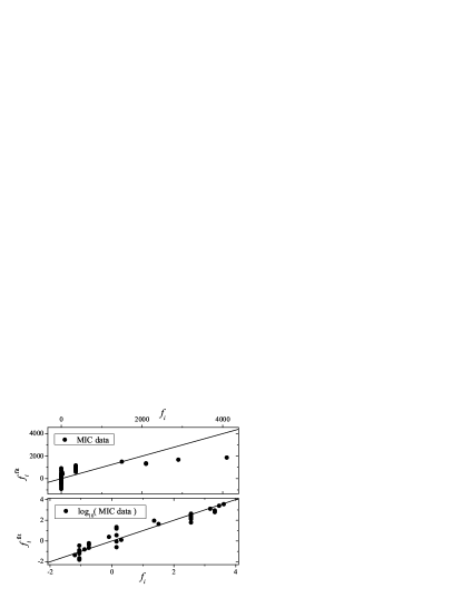
Figure 3: The measured fitness values, $f_{i}$, for the $\beta$-lactamase resistance landscape E [57] are plotted vs. the fitness values obtained from the fit with the model described by equation (3), $f_{i}^{\mathrm{fit}}$. For a perfect fit, all dots would lie on the straight line with slope 1. The upper panel uses the measurements taken directly from [57]. A systematic deviation from the straight line is observed. The lower panel uses the logarithms of the measurements; no systematic deviations are observed.

In the datasets H-J, fitness proxies are missing for several genotypes (table 1). The cause is either non-viability of those genotypes (dataset H) or unobserved genotypes (dataset I-J). In the latter case, we assume that the unobserved genotypes were missed by chance [60]. We therefore replaced the missing measurements by values obtained from the fitted multidimensional linear model and subsequently performed the logarithmic transformation. The presence of non-viable genotypes poses a problem for the log transformation of the fitness measurements. Dataset H was shown to contain non-viable A. niger genotypes on the basis of a statistical analysis [30]. A non-viable genotype would imply a logarithmic fitness equal to minus infinity. To circumvent this issue, we did not perform the log transformation for this dataset. Because the fitness values of viable genotypes (expressed in terms of relative growth rates) were fairly close to unity, taking the logarithm of the fitness values of viable genotypes would not substantially alter the results.

The results of the standardized analyses are presented in table 2. In short, we observe that landscapes obtained by combining genome-wide mutations with a known collectively beneficial effect are more smooth. In fact, the landscapes A and B share these two characteristics and have the lowest ruggedness for all four measures (see fig. 4). The landscapes obtained by combining mutations with a known beneficial effect from a single gene (data sets C-F) are more rugged, while the highest degree of ruggedness is measured in landscapes constructed from genome-wide mutations with deleterious (data sets G and H) or unknown (data sets I and J) effects. Before turning to the biological implications of these trends in sect. 4, we find it useful to establish the correlation between the different measures (sect. 3.2.3) and the fit to the RMF model (sect. 3.2.4).

Table 2: Quantitative measures of ruggedness and epistasis for 10 empirical fitness landscapes. Except for the landscapes of size $L=4$, the reported values are averages over all possible 4-locus subgraphs. The last two lines show reference values obtained from simulations of the house-of-cards model with $L=4$ (HoC), and for a perfectly additive landscape (PA).

ID	Ref.	$L$	$r/s$	$F_{1}$	$F_{2}$	$F_{\mathrm{sum}}$	$N_{\mathrm{max}}$	$N_{\mathrm{cp}}$	$f_{\mathrm{r}}$	$f_{\mathrm{s}}$	$f_{\mathrm{mm}}$
A	[26]	4	0.122	0.989	0.009	0.011	1	24	0	0	1
B	[56]	5	0.290	0.942	0.040	0.058	1.10	16.80	0.013	0.150	1.92
C	[27]a	4	0.517	0.267	0.400	0.733	2	16	0.083	0.250	0.67
D	[27]b	4	0.986	0.537	0.197	0.463	2	10	0.125	0.458	0.67
E	[57]	5	0.418	0.894	0.064	0.106	1.50	6.53	0.025	0.150	1.09
F	[58]c	5	0.380	0.921	0.061	0.079	1.30	8.75	0.050	0.250	3.03
G	[59]	6	1.180	0.658	0.179	0.342	2.13	2.10	0.229	0.358	3.16
H	[30]	8	1.304	0.547	0.269	0.453	2.61	2.31	0.154	0.262	2.19
I	[60]d	9	1.317	0.376	0.368	0.624	2.66	2.02	0.240	0.292	1.71
J	[60]e	9	1.199	0.383	0.372	0.617	2.48	2.51	0.227	0.300	1.92
•	HoC	4	2.423	0.267	0.402	0.733	3.20	1	0.333	0.333	2.20
□	PA	4	0	1	0	0	1	24	0	0	1

• Pyrimethamine resistance measurements.

• Growth rate measurements.

• Data for piperacillin resistance in the presence of a $\beta$-lactamase inhibitor; these mutations were originally selected for their beneficial effect on cefotaxime resistance [57].

• Relative 5-epi-Aristolochene output (main product of TEAS terpene synthase).

• Relative Premnaspirodiene output (main product of HPS terpene synthase).

3.2.3 Correlation between different measures of landscape ruggedness.

To investigate how well the different measures (except $f_{\mathrm{mm}}$) correlate to one another, we first rank all landscapes for each measure separately; i.e., if a landscape has the $n$-th lowest value for a quantity, it is assigned rank $n$ with respect to that quantity. In fig. 4, we make pairwise plots of these ranks for the different measures. For a perfect rank correlation between the measures, the symbols should lie on a straight line. In general, the different measures of ruggedness correlate well, suggesting that these quantities all reflect the relative contribution of epistasis in a similar way. The number of maxima $N_{\mathrm{max}}$ even has a perfect rank correlation with the roughness to slope ratio $r/s$. The number of crossing paths, $N_{\mathrm{cp}}$, correlates somewhat less well with the other quantities. We will examine this deviation when we compare the measured values with expectations from model landscapes.

Figure 4: The ranks of the fitness landscapes specified in table 2 with respect to the studied quantifiers of epistasis are plotted against each other. In general, the quantities seem rather well correlated (see main text for a detailed discussion).

It is also instructive to compare data sets that measure different quantities using the same set of genotypes. Landscapes C and D are based on measurements of drug resistance and growth rate, respectively. The mutations in this set of genotypes were selected for their beneficial effects on resistance. Increased resistance is expected to have a trade-off in the absence of the drug and since growth rates were determined under these conditions, the included mutations are no longer beneficial. Given the tendency that landscapes from beneficial mutations are more smooth, it is not surprising that the growth rate landscape D is more rugged than the resistance landscape C. Landscapes E and F are based on a genotype with multiple mutations that is selected because of the increased resistance to a particular $\beta$-lactam antibiotic, cefotaxime. The fitness proxy used to construct landscape E is cefotaxime resistance, whereas in landscape F it is resistance to another antibiotic, piperacillin, which was not involved in the selection of the genotypes. However, the reason why they were measured in the piperacillin environment (with inhibitor) is because resistance in this environment showed an overall trade-off with cefotaxime resistance. Hence, the included (reverse) mutations were collectively beneficial for this environment. In contrast to landscapes C and D, the landscapes E and F turn out to be almost equally rugged.

Figure 5: The measured values for the studied quantifiers of epistasis are plotted with respect to each other for the fitness landscapes specified in table 2. The black line corresponds to values obtained numerically for RMF landscapes interpolating between a non-epistatic (open square) and a completely random (filled circle) landscape.

3.2.4 Combining models and empirical data.

To compare the measurements for the empirical landscapes with expectations calculated for model landscapes, we use the predictions generated by the RMF model (2). We thereby fixed the parameter controlling the roughness of the landscape to $a=0.01$, and calculated all measures for various choices of the slope $c$. For each pair of $a$ and $c$, the calculated values were averaged over 10,000 realizations of the 4-locus landscape. Recall that the case $c=0$ corresponds to a completely random landscape, i.e. to the House-of-Cards model. The opposite extreme of a purely additive landscape was also considered by setting $a=0$ for an arbitrary value of $c\neq 0$.

In fig. 5, we plot all pairwise combinations of the four epistasis measures previously included in the rank analysis of fig. 4. The black line corresponds to the range of possible outcomes for the model landscapes, one limit corresponding to the House-of-Cards case (marked by a filled circle) and the other limit being the purely additive case (marked by an empty square). The letters represent the measurements from the experimental landscapes (see table 2). The close correspondence between the letters and the line indicates that the RMF model captures the different ruggedness measures and their correlations observed for the experimental landscapes surprisingly well. The relatively large deviations for landscapes C and D from [27] are most likely due to the fact that this is a 4-locus landscape and measurements are thus based on a single observation, rather than being an average over multiple subgraphs of size $m=4$ as is the case for the larger landscapes. We also note that the number of crossing paths $N_{\mathrm{cp}}$ observed in the empirical landscapes appears to be systematically smaller than predicted by the RMF model, a deviation which coincides with the relatively low rank correlation of this measure compared to the other measures (fig. 4).

4 Discussion and outlook

In this review, we have first established a set of standardized measures to determine the ruggedness of fitness landscapes. We then use these measures to compare the ruggedness of ten available empirical landscapes, and to compare the empirical landscapes to predictions generated by the Rough Mount Fuji (RMF) model, a model with tunable ruggedness. Our rank analyses show that the selected measures correlate very well, and thus appear to capture the same underlying feature of the landscape. In a sense, they all capture the amount of epistasis in a particular landscape. What is quite remarkable is that not all measures are sensitive to detect all types of epistasis. The Fourier analysis and the $r/s$ ratio are sensitive to magnitude epistasis, sign epistasis and reciprocal sign epistasis. The local epistasis measure, $f_{r}+f_{s}$, and measures of accessible pathways are insensitive to magnitude epistasis, while the number of local fitness maxima is only sensitive to detect reciprocal sign epistasis. The fact that the rank correlations between the different measures are still high could either mean that the effects of sign epistasis dominate the measures that are sensitive to magnitude epistasis or that the three types of epistasis co-occur. The above also implies that the measure of epistasis among two loci ($f_{r}+f_{s}$) contains similar information as the more global measures of epistasis (involving 4 loci). Sampling local interactions can be done by detection of pairwise interactions between mutations, which is experimentally more straightforward than building multidimensional landscapes of connected genotypes. On the other hand, the Fourier analysis shows that higher-order interactions between mutations ($F_{3},F_{4}$, etc.) play a significant role, especially in the more rugged landscapes. This information can only be detected by the construction of such landscapes.

Before we discuss which characteristics of mutations are either linked with smooth or rugged landscapes, we need to emphasize that the small number of available landscapes only allows for preliminary conclusions and that the comparison is complicated by differences in the methodologies involved to measure fitness. Nevertheless, general patterns do emerge as well as gaps in our knowledge. All empirical landscapes are relatively small in size and a specific set of mutations is used to construct the genotypes. These mutations fall into different classes. Unfortunately, few representatives are available per class, and worse: we lack any data for other classes. For example, no landscapes are available using mutations known to be beneficial by themselves in a particular wildtype, nor do we know of any studies that constructed landscapes from deleterious mutations in a single gene. This necessarily limits the interpretation and generality of our findings.

A first characteristic of a mutation which affects ruggedness is whether the mutation is deleterious [30, 59] or beneficial [27, 26, 56, 60, 57]. Among the available landscapes, those that are constructed using beneficial mutations (A-C and E-F in Table 2) are smoother than those using deleterious mutations (G-H). Although beneficial mutations are much rarer than deleterious ones [54, 78], most studies focus on beneficial mutations. This seems justified given that beneficial mutations do account for a large fraction of the mutations that contribute to long-term evolution [79, 80]. Both types of mutations are intrinsically linked, since each fixed beneficial mutation becomes a potential deleterious mutation when the direction of selection reverses. In that global sense, it does not matter which type we are dealing with. However, there is the possibility that deleterious and beneficial mutations have intrinsically different statistical properties, including epistatic interactions, because they sample different parts of the local fitness landscape. Similarly, the position of the wild type is of influence. For example, the beneficial mutations in the TEM-1 $\beta$-lactamase fitness landscape E increase resistance to the antibiotic cefotaxime [57]. The TEM-1 wild type incurs a very low resistance towards this antibiotic, and the fittest genotype has approximately a 100,000-fold higher resistance. This clearly differs from the study by Chou et al. [26] (landscape A) in which a new metabolic pathway is introduced into a strain of Methylobacterium extorquens and the fittest genotype displays a $94\%$ (i.e. $\sim 2$-fold) fitness increase. Note also that the empirical fitness landscapes include mutations that are known to alter fitness (individually or collectively), and mutations with an individually neutral effect are excluded. Still, neutral mutations make up a significant portion of all available mutations [81], and are known to contribute to long-term adaptation [8].

A second characteristic that appears to influence the degree of ruggedness is whether the individual or the combined effect (beneficial or deleterious) is known. For example, the mutations that were studied by Chou et al. [26] and Khan et al. [56] (landscape B) collectively produced a well-adapted genotype after many generations of evolution, whereas the mutations studied by [30] (landscape H) were a priori only known to have a deleterious effect in the wild-type background. In the first category, all intermediates are constructed between two points in genotype space that are connected by at least one accessible pathway (otherwise the higher-fitness genotype would not have been found). In the second category, the genotype that combines all mutations is not necessarily accessible from the wildtype, and does not even have to be better adapted. Consistent with an expected greater bias against (sign) epistasis in the first category, the landscapes based on genome-wide collectively beneficial mutations show less epistasis than those based on individually deleterious mutations (see table 2). A better direct test would be a comparison between mutations with known collective or individual effect of the same fitness sign (all beneficial or all deleterious) within the same biological system, but we presently lack such data.

A third distinction that affects ruggedness of empirical fitness landscapes is the level at which the mutations interact. The included mutations can for example affect fitness [30, 56], can operate in a common genetic pathway [26], or can even be located in the same gene [27, 58, 57]. The landscapes constructed from beneficial mutations located in different genes (A-B) are smoother than those from beneficial mutations located in the same gene (C and E-F). When epistasis is detected between mutations in different genes, this information has traditionally been used to infer their combined contribution to a metabolic pathway. The reverse is also true: when empirical fitness landscapes combine mutations that operate in a common genetic pathway, finding epistasis becomes more likely. This becomes even more prominent when mutations are located in a single gene. Epistasis among mutations in different genes can result from functional constraints caused by interactions in a metabolic network [82, 83], whereas intragenic epistasis can also result from structural constraints when nucleotide positions in a single gene have a combined effect on protein shape, enzyme activity, or folding-stability [84, 85]. This relates to the type of epistasis that one expects to find. Magnitude epistasis is often associated with mutations in different genes in a metabolic network [54, 86, 87], whereas sign epistasis is expected to occur more often between positions in a single gene [88]. The expectation of a greater contribution of epistasis to landscapes based on mutations in a single gene versus in different genes is supported by our analysis (see table 2). Note however, that compensatory mutations are often located in different genes [53, 89], and that sign epistasis between deleterious mutations has also been shown to occur at a genome-wide scale [30].

Having in mind all complicating differences between the various fitness proxies and the diverse set of biological organisms used for testing, it is all the more surprising how well the simple model (2) seems to capture features of the real landscapes. However, we emphasize that we studied averaged quantities of small (i.e. 4-locus) subgraphs of the landscapes in order to standardize our measures and compare them to model predictions. Hence information contained in the full landscape might have been overlooked in these analyses. For example, the considerations in the previous paragraph suggest that the level of interaction between mutants should be distributed very inhomogeneously on large enough landscapes, consistent with predictions from metabolic models [1, 83]. This means that the landscapes can be decomposed into subgraphs, some of which contain much, others little or no epistasis. Such a decomposition would reflect the strength of interactions between specific combinations of mutations. For instance, one would expect that mutations changing the same functional part of one protein should highly influence the impact of one another on the function. On the other hand, the impact of mutations altering different proteins, which do not interact, should be independent of each other. Searching for such patterns by looking at distributions of epistasis measures instead of their mean, is a promising direction for future study.

If the existence of genetic modules with different levels of epistasis can be established empirically, it will be a challenge for future models of fitness landscapes to take this realism into account, and study its evolutionary consequences. In fact, the $LK$ model [27, 28] was introduced with the idea of incorporating such structures. However, these models make very specific assumptions about the distribution of the size and coupling of different epistastic modules, and these should be compared to measures based on empirical landscapes. Where systematic deviations are observed, the empirical information may then be used to adapt the models. Much of the progress in understanding fitness landscapes and their evolutionary implications, therefore, depends on the availability of additional empirical landscapes from various systems – particularly from those classes where we lack any information.

References

References

- [1] Costanzo M, Baryshnikova A, Bellay J, Kim Y, Spear E D et al. 2010 Science 327 425–431
- [2] de Visser J A G M, Cooper T F and Elena S F 2011 Proc. R. Soc. Lond. [Biol] 278 3617–3624
- [3] Wagner G P and Zhang J 2011 Nat. Rev. Genet. 12 204–213
- [4] Haldane J B S 1931 Proc. Cambridge Philos. Soc. 27 137–142
- [5] Wright S 1932 Proc. IV Int. Cong. Genet. 1 356–366
- [6] Carneiro M and Hartl D L 2009 Proc. Natl. Acad. Sci. USA 107 1747–1751
- [7] Jain K and Krug J 2007 Genetics 175 1275–1288
- [8] Wagner A 2008 Nat. Rev. Genet. 9 965–974
- [9] Phillips P C 2008 Nat. Rev. Genet. 9 855–867
- [10] Wolf J B, Brodie E D and Wade M J 2000 Epistasis and the evolutionary process (Oxford: Oxford University press)
- [11] Gavrilets S 2004 Fitness landscapes and the origin of species (Princeton: Princeton University Press)
- [12] Kondrashov F A and Kondrashov A S 2001 Proc. Natl. Acad. Sci. USA 98 12089–12092
- [13] de Visser J A G M, Park S-C and Krug J 2009 Am. Nat., 174, S15–S30
- [14] Otto S P 2009 Am. Nat. 174 S1–S14
- [15] Lenski R E, Barrick J E and Ofria C 2006 PLoS Biol. 4 e428
- [16] van Nimwegen E, Crutchfield J P and Huynen M 1999 Proc. Natl. Acad. Sci. USA 96 9716–9720
- [17] Wagner A 2005 Robustness and evolvability in living systems (Princeton Studies in Complexity) (Princeton: Princeton University Press)
- [18] Lobkovsky A E, Wolf Y I and Koonin E V 2011 PLoS Comput. Biol. 7 e1002302
- [19] Salverda M L M, Dellus E, Gorter F A, Debets A J M, Van der Oost J, Hoekstra R F, Tawfik D S et al. 2011 PLoS Genet. 7 e1001321
- [20] Colegrave N and Buckling A 2005 BioEssays 27 1167–1173
- [21] Fisher R A 1918 Trans. R. Soc. Edinb. 52 399–433
- [22] Weinreich D M, Watson R A and Chao L 2005 Evolution 59 1165–1174
- [23] Poelwijk F J, Kiviet D J, Weinreich D M and Tans S J 2007 Nature 445 383–386
- [24] Poelwijk F J, Tanase-Nicola S, Kiviet D J, Tans S J 2011 J Theor. Biol. 272 141.
- [25] de Visser J A G M, Hoekstra R F and van den Ende H 1997 Evolution 51 1499–1505
- [26] Chou H-H, Chiu H-C, Delaney N F, Segrè D and Marx C J 2011 Science 332 1190–1192
- [27] Lozovsky E R, Chookajorn T, Browna K M, Imwong M, Shaw P J, Kamchonwongpaisan S, Neafsey D E et al. 2009 Proc. Natl. Acad. Sci. USA 106 12015–12030
- [28] Kauffman SA, Weinberger ED 1989 J. Theor. Biol. 141 211-245.
- [29] Kauffman S A 1993 The origins of order: Self-Organization and Selection in Evolution (New York: Oxford University Press)
- [30] Franke, J, Klözer A, de Visser J A G M and Krug J 2011 PLoS Comput. Biol. 7 e1002134
- [31] Weinberger E D 1996 -Completeness of Kauffman’s NK Model: A Tunably Rugged Fitness Landscape Santa Fe Institute Working Paper 96-02-003
- [32] Kingman J F C 1978 J. Appl. Probab. 15 1–12
- [33] Derrida B 1981 Phys. Rev. B 24 2613–2626
- [34] Aita T, Uchiyama H, Inaoka T, Nakajima M, Kokubo T and Husimi Y 2000 Biopolymers 54 64–79
- [35] Stauffer D and Aharony A 1991 Introduction to Percolation Theory, (London and Philadelphia: Taylor and Francis)
- [36] Gavrilets S and Gravner J 1997 J. Theor. Biol. 184 51–64
- [37] Khatri B S, McLeish T C B and Sear R P 2009 Proc. Natl. Acad. Sci. USA 106 9564–9569
- [38] Fontana W, Stadler P F, Bornberg-Bauer E G, Griesmacher T, Hofacker I L, Tacker M, Tarazona P, Weinberger E D and Schuster P 1993 Phys. Rev. E 47 2083–2099
- [39] Mustonen V, Kinney J, Callan Jr C G and Lässig M 2008 Proc. Natl. Acad. Sci. USA 105 12376–12381
- [40] Elena S F and Lenski R E 2003 Nat. Rev. Genet. 4 457–469
- [41] Korona R, Nakatsu C H, Forney L J and Lenski R E 1994 Proc. Natl. Acad. Sci. USA 91 9037–9041
- [42] Rozen D E, Habets M G J L, Handel A and de Visser J A G M 2008 PLoS One 3 e1715
- [43] Burch C L and Chao L 2000 Nature 406 625–628
- [44] van Opijnen T, de Ronde A, Boerlijst M C and Berkhout B 2007 PLoS One 2 e271
- [45] Buckling A, Wills M A and Colegrave N 2003 Science 302 2107–2109
- [46] Gifford D R, Schoustra S E and Kassen R 2011 Evolution 65 3070–3078
- [47] Schoustra S E, Bataillon T, Gifford D R and Kassen R 2009 PLoS Biol. 7 e1000250
- [48] Orr HA 2003 J. theor. Biol. 220, 241–247
- [49] Neidhart J and Krug J 2011 Phys. Rev. Lett. 107 178102
- [50] Park S-C, Simon D and Krug J 2010 J. Stat. Phys. 138, 381–410
- [51] Blount Z D, Borland C Z and Lenski R E 2008 Proc. Natl. Acad. Sci. USA 105 7899–7906
- [52] Woods R J, Barrick J E, Cooper T F, Shrestha U, Kauth M R and Lenski R E 2011 Science 331 1433–1436
- [53] Rokyta D R, Joyce P, Caudle S B, Miller C, Beisel C J and Wichman H A 2011 PLoS Genet. 7 e1002075
- [54] Sanjúan R, Moya A and Elena S F 2004 Proc. Natl. Acad. Sci. USA 101 15376–15379
- [55] Hinkley T, Martins J, Chappey C, Haddad M, Stawiski E, Whitcomb J M, Petropoulos C J et al. 2011 Nat. Genet. 43 487–490
- [56] Khan A I, Dinh D M, Schneider D, Lenski R E and Cooper T F 2011 Science 332 1193–1196
- [57] Weinreich D M, Delaney N F, DePristo M A and Hartl D L 2006 Science 312 111–114
- [58] Tan L, Serene S, Chao H X and Gore J 2011 Phys. Rev. Lett. 106 198102
- [59] Hall D W, Agan M and Pope S C 2010 J. Hered. 101 S75–S84
- [60] O’Maille P E, Malone A, Dellas N, Hess Jr B A, Smentek L, Sheehan I, Greenhagen B T et al. 2008 Nat. Chem. Biol. 4 617–623
- [61] Brown K M, Costanzo M S, Xu W, Roy S, Lozovsky E R and Hartl D L 2010 Mol. Biol. Evol. 27 2682–2690
- [62] Costanzo M S, Brown K M and Hartl D L 2011 PLoS ONE 6 e19636
- [63] da Silva J, Coetzer M, Nedellec R, Pastore C and Mosier D E 2010 Genetics 185 293–303
- [64] Lunzer, M, Miller S P, Felsheim R and Dean A M 2005 Science 310 499–501
- [65] Aita T, Iwakura M and Husimi Y 2001 Protein Eng. 14 633–638
- [66] Stadler P F 1996 J. Math. Chem. 20 1–45
- [67] Neher R A and Shraiman B I 2011 Rev. Mod. Phys. 83 1283–1300
- [68] Kauffman S and Levin S 1987 J. Theor. Biol. 128 11–45
- [69] Rosenberg N A 2005 J. Theor. Biol. 237 17–22
- [70] Weinberger E D 1989 Phys. Rev. A 44 6399–6413
- [71] Durrett R and Limic V 2003 Ann. Prob. 31 1713–1753
- [72] Limic V and Pemantle R 2004 Ann. Prob. 32 2149–2178
- [73] Neidhart J 2011 Adaptive walks in random and correlated fitness landscapes Master thesis, University of Cologne
- [74] DePristo M A, Hartl D L and Weinreich D M 2007 Mol. Biol. Evol. 24(8) 1608–1610
- [75] Roy S W 2009 PLoS One 4 e4500
- [76] Stadler P F 2002 Biological Evolution and Statistical Physics (Lecture notes in physics) ed M Lässig and A Valleriani (Berlin: Springer)
- [77] Achaz G (private communication)
- [78] Perfeito L, Fernandes L, Mota C and Gordo I 2007 Science 317 813–815
- [79] Smith N G Eyre-Walker A 2002 Nature 415 1022–1024
- [80] Welch JJ (2006) Genetics 173 821–837
- [81] Eyre-Walker A and Keightley P D 2007 Nat. Rev. Genet. 8 610–618
- [82] Szathmáry E 1993 Genetics 133 127–132
- [83] Segrè D, DeLuna A, Church G M and Kishony R 2005 Nat. Genet. 37 77–83
- [84] DePristo M A, Weinreich D M and Hartl D L 2005 Nat. Rev. Genet. 6 678–687
- [85] Wang X, Minasov G and Shoichet B K 2002 J. Mol. Biol. 320 85–95
- [86] Jasnos L and Korona M 2007 Nat. Genet. 39 550–554
- [87] Burch C L and Chao L 2004 Genetics 167 559–567
- [88] Watson R A, Weinreich D M and Wakeley J 2011 Evolution 65 523–536
- [89] Poon A and Chao L 2005 Genetics 170 989–999