Linear approach to the orbiting spacecraft thermal problem

Abstract

We develop a linear method for solving the nonlinear differential equations of a lumped-parameter thermal model of a spacecraft moving in a closed orbit. Our method, based on perturbation theory, is compared with heuristic linearizations of the same equations. The essential feature of the linear approach is that it provides a decomposition in thermal modes, like the decomposition of mechanical vibrations in normal modes. The stationary periodic solution of the linear equations can be alternately expressed as an explicit integral or as a Fourier series. We apply our method to a minimal thermal model of a satellite with ten isothermal parts (nodes) and we compare the method with direct numerical integration of the nonlinear equations. We briefly study the computational complexity of our method for general thermal models of orbiting spacecraft and conclude that it is certainly useful for reduced models and conceptual design but it can also be more efficient than the direct integration of the equations for large models. The results of the Fourier series computations for the ten-node satellite model show that the periodic solution at the second perturbative order is sufficiently accurate.

Nomenclature

$A_{i}$	=	outward-facing area of ith-node, m2
$C$	=	thermal capacitance diagonal matrix, J/K
$C_{i}$	=	thermal capacitance of ith-node, J/K
$e_{a}$	=	eigenvector of $C^{1/2}JC^{-1/2}$, K
$e_{aj}$	=	jth-component of eigenvector $e_{a}$, K
$F(t)$	=	driving function vector, K/s
$\hat{F}(m)$	=	$m$th Fourier coefficient of $F(t)$, K/s
$\hat{F}^{*}$	=	complex conjugate of $\hat{F}$, K/s
$F_{a}(t)$	=	driving function for $a$th-mode, K/s
$\dot{F}_{a}(t)$	=	time derivative of $F_{a}(t)$, K/s2
$F_{i}(t)$	=	driving function for $i$th-node, K/s
$\hat{F}_{i}(m)$	=	$m$th Fourier coefficient of $F_{i}(t)$, K/s
$G(t)$	=	driving function for second order temperature vector, K/s
$J$	=	Jacobian matrix, s-1
$J_{ij}$	=	Jacobian matrix ij-element, s-1
$k$	=	number of steps in numerical integration of ODEs
$K$	=	conduction coupling matrix, W/K
$K^{R}$	=	matrix of conductances from linearized radiation coupling terms, W/K
$K_{i}^{R}$	=	$i$th-node conductance from linearized environment-radiation terms, W/K
$K_{ij}$	=	conduction coupling matrix ij-element, W/K
$K_{ij}^{R}$	=	ij-element of conductance matrix from linearized radiation terms, W/K
$n$	=	number of samples for discrete Fourier transform
$N$	=	number of nodes
$P$	=	eigenvector matrix for J, K
$P_{ia}$	=	ith-component of $J$-eigenvector for $a$th-mode, K
$q$	=	auxiliary heat input vector, K/s
$\dot{Q}_{i}(t)$	=	heat input to ith-node, W
$\langle\dot{Q}_{i}\rangle$	=	mean value of $\dot{Q}_{i}(t)$ over period $\cal{T}$, W
$R_{i}$	=	ith-node coefficient of radiation to the environment, W/K4
$R_{ij}$	=	radiation coupling matrix, W/K4
$t$	=	time, s (min in figures)
$T$	=	temperature vector, K
$\Delta T$	=	vector of “errors” w.r.t. ESATANTM solution, K
$\widetilde{T}$	=	steady-state temperature vector, K
$T_{i}$	=	temperature of i-node, K
$T_{0}$	=	cosmic microwave background radiation temperature, K
$T_{(n)j}$	=	nth order term in jth-node temperature expansion, K
$T^{\infty}$	=	stationary solution temperature vector, K
$T^{\infty}_{(n)}$	=	nth order of stationary solution temperature vector, K
$\dot{T}_{i}$	=	time derivative of ith-node temperature, K/s
$\widetilde{T}_{i}$	=	steady-state temperature of ith-node, K
$\cal{T}$	=	orbital period, s
$U$	=	matrix of independent solutions to homogeneous equations, K
$\alpha_{s}$	=	solar absorptivity
$\delta_{ab}$	=	Kronecker’s delta
$\delta A$	=	antisymmetric part of $C^{1/2}JC^{-1/2}$, s-1
$\delta A_{ij}$	=	ij-element of $\delta A$, s-1
$\varepsilon_{i}$	=	infrared emissivity of ith-node outward-facing surface
$\epsilon$	=	perturbation parameter
$\lambda_{a}$	=	eigenvalue of J for $a$th mode, s-1
$\delta\lambda_{a}$	=	perturbation of J-eigenvalue for $a$th mode, s-1
$\sigma$	=	Stefan-Boltzmann constant, $5.67\times 10^{-8}$ W m${}^{-2}\,$K-4

I Introduction

The thermal control of a spacecraft ensures that the temperatures of its various parts are kept within their appropriate ranges Kreith ; therm-control ; therm-control_2 ; therm-control_3 . The simulation and prediction of temperatures in a spacecraft during a mission are usually carried out by commercial software packages. These software packages employ “lumped parameter” models that describe the spacecraft as a discrete network of nodes, with one energy-balance equation per node. The equations for the thermal state evolution are coupled nonlinear first-order differential equations, which can be integrated numerically. Given the thermal parameters of the model and its initial thermal state, the numerical integration of the differential equations yields the solution of the problem, namely, the evolution of the node temperatures. However, a detailed model with many nodes is difficult to handle, and its integration for a sufficiently long time of evolution can take considerable computer time and resources. Therefore, it is very useful to study simplified models and approximate methods of integrating the differential equations.

Many spacecraft missions, in particular, satellite missions, consist of an initial transient part and then a stationary part, in which the spacecraft just goes around a closed orbit, in which the heat inputs are periodic. These periodic heat inputs are expected to induce periodic temperature variations, with a maximum and a minimum temperature in each orbit. This suggests a conservative approach that consists in computing only the temperatures for the hot and cold cases of the given orbit, defining them as the two steady cases with the maximum and minimum heat loads, respectively. Naturally, the real temperature variations in the orbit are smaller, because there is not enough time for the hot and cold cases to establish themselves. In fact, the temperature variations can be considerably smaller, to such a degree that it is necessary to integrate the differential equations, at least approximately.

The differential equations for energy balance are nonlinear due to the presence of radiation couplings, which follow the Stefan-Boltzmann quartic law. A common approach to these equations involves a linearization of the radiation terms that approximate them by heat conduction terms anal-sat ; therm-control_2 ; anal-sat_2 ; IDR . This approach transforms the nonlinear equations into standard linear heat conduction equations. But this approach has not been sufficiently justified, is of a heuristic nature and does not constitute a systematic approximation.

In fact, nonlinear equations are very different from linear equations and, in particular, a periodic driving may not induce periodic solutions but much more complex solutions, namely, chaotic solutions. Therefore, we have carried out in preceding papers a full nonlinear analysis of spacecraft thermal models NoDy ; NoDy1 . The conclusion of the analysis is that the complexities of nonlinear dynamics, such as multiple equilibria and chaos, do not appear in these models. While the existence of only one equilibrium state can be proved in general, the absence of chaos under driving by variable external heat loads can only be proved for a limited range of magnitudes of the driving loads. This range presumably includes the magnitudes involved in typical spacecraft orbits. The proofs in Refs. 9 and 10 are constructive and are based on a perturbation method that is expected to be sound when the linear equations corresponding to the first perturbative order constitute a good approximation of the nonlinear equations. This implies that the fully nonlinear solution describes a weakly nonlinear oscillator. Since the perturbative approximation is mathematically rigorous and systematic, it is worthwhile to study in detail the scope of the perturbative linear equations and, furthermore, to compare them with previous linear approaches of a heuristic nature.

The main purpose of this paper is to study the linear method of predicting the thermal behavior of spacecraft in stationary orbits (Sect. II and III) and to test it on a minimally realistic thermal model of a satellite in a circular orbit. Since the general one and two-node models analyzed in Refs. 9 and 10, respectively, are too simple, we define in this paper a ten-node thermal model of a small Moon-orbiting satellite (Sect. IV). This model is simple enough to allow us to explicitly show all the quantities involved (thermal couplings and capacities, heat inputs, etc.) and it is sufficient for illustrating the main features of the linear approach. As realistic thermal models have many more nodes, we consider in Sect. V the important issue of scalability of the method and, hence, its practical applications. Computational aspects of the steady-state problem have been studied by Krishnaprakas Kris1 ; Kris2 and by Milman and Petrick MiPe , while computational aspects of the direct integration of the nonlinear equations for the unsteady problem have been studied by Krishnaprakas Kris3 . Here we focus on the linear equations for the stationary but unsteady case and survey its computational aspects.

A note on notation: In the equations that contain matrix or vector quantities, sometimes we use component notation (with indices) while other times we use compact matrix notation (without indices), according to the nature of the equations.

II Linearization of the heat-balance equations

A lumped-parameter thermal model of a continuous system consists of a discrete network of isothermal regions (nodes) that represent a partition of the total thermal capacitance and that are linked by thermal conduction and radiation couplings Kreith ; therm-control ; therm-control_2 ; therm-control_3 ; anal-sat . This discretization reduces the integro-differential heat-transfer equations to a set of energy-balance ODEs, one per node, which control the evolution of the nodes’ temperatures anal-sat :

$$C_{i}\,\dot{T_{i}}=\dot{Q}_{i}(t)-\sum_{j=1}^{N}\left[K_{ij}(T_{i}-T_{j})+R_{ij}(T_{i}^{4}-T_{j}^{4})\right]-R_{i}\,({T_{i}}^{4}-T_{0}^{4}),\quad i=1,\ldots,N,$$ (1)

where $N$ is the number of nodes and $\dot{Q}_{i}(t)$ contains the total heat input to the $i$th-node from external radiation and from internal energy dissipation (if there is any). The conduction and radiation coupling matrices are denoted by $K$ and $R$, respectively; they are symmetric ($K_{ij}=K_{ji}$ and $R_{ij}=R_{ji}$) and $K_{ii}=R_{ii}=0$; so there are $N(N-1)$ independent coupling coefficients altogether, but many vanish, usually. The temperature $T_{0}\simeq 3\!$ K is the temperature of the environment, namely, the cosmic microwave background radiation. The $i$th-node coefficient of radiation to the environment is given by $R_{i}=A_{i}\varepsilon_{i}\sigma$, where $A_{i}$ denotes the outward facing area, $\varepsilon_{i}$ its (infrared) emissivity, and $\sigma$ is the Stefan-Boltzmann constant. The constant term $R_{i}T_{0}^{4}$ can be included in $\dot{Q}_{i}(t)$ or ignored altogether, if each ${T_{i}}\gg T_{0}$. Equations (1) coincide with the ones implemented in commercial software packages, for example, ESATAN^TM ESATAN .

There is no systematic procedure for finding the analytical solution of a system of nonlinear differential equations, except in some particularly simple cases. Of course, nonlinear systems can always be integrated numerically with finite difference schemes. Methods of this kind are employed in commercial software packages. When a nonlinear system can be approximated by a linear system and, hence, an approximate analytic solution can be found, this solution constitutes a valuable tool. Actually, one can always resort to some kind of perturbation method to linearize a nonlinear system. Therefore, we now study the rigorous linearization of Eqs. (1) based on a suitable perturbation method, and we also describe, for the sake of a comparison, a heuristic linearization, which actually is best understood in light of the results of the perturbation method.

II.1 Perturbative linearization

If we assume that the heat inputs $\dot{Q_{i}}(t)$ in the energy-balance Eqs. (1) are periodic, namely, that there is a time interval ${\cal T}$ such that $\dot{Q_{i}}(t+{\cal T})=\dot{Q_{i}}(t)$, then it seems sensible to study first the effect of the mean heat inputs in a period. This averaging method, introduced in Refs. 9 and 10, relies on the fact that the autonomous nonlinear system of ODEs for constant $\dot{Q_{i}}$ can be thoroughly analyzed with analytical and numerical methods. For example, it is possible to determine that there is a unique steady thermal state and that it is (locally) stable MiPe ; NoDy1 . The actual values of the steady temperatures can be found efficiently with various numerical methods Kris1 ; Kris2 ; MiPe . Furthermore, the eigenvalues and eigenvectors of the Jacobian matrix of the nonlinear system of ODEs provides us with useful information about the dynamics, in particular, about the approach to steady-state: the eigenvectors represent independent thermal modes and the eigenvalues represent their relaxation times NoDy1 .

Once the averaged equations are solved, the variation of the heat inputs can be considered as a driving of the averaged solutions. Thus, we can define the driving function

$$F_{i}(t)=\frac{\dot{Q_{i}}(t)-\langle{\dot{Q_{i}}}\rangle}{C_{i}}\,,\quad i=1,\ldots,N,$$

where $\langle{\dot{Q_{i}}}\rangle$ denotes the mean value of $\dot{Q_{i}}(t)$ over the period of oscillation. A weak driving function must not produce a notable deviation from the averaged dynamics. In particular, the long-term thermal state of an orbiting spacecraft must oscillate about the corresponding steady-state. To embody this idea, we introduce a formal perturbation parameter $\epsilon$, to be set to the value of unity at the end, and write Eqs. (1) as

$$\dot{T}_{i}=\epsilon\,F_{i}(t)+\frac{\langle{\dot{Q_{i}}}\rangle}{C_{i}}-\sum_{j=1}^{N}\left[\frac{K_{ij}}{C_{i}}(T_{i}-T_{j})+\frac{R_{ij}}{C_{i}}(T_{i}^{4}-T_{j}^{4})\right]-\frac{R_{i}}{C_{i}}\,{T_{i}}^{4},\quad i=1,\ldots,N,$$ (2)

Then, we assume an expansion of the form

$$T_{j}(t)=\sum_{n=0}^{\infty}\epsilon^{n}\,T_{(n)j}(t)\,.$$ (3)

When we substitute this expansion into Eqs. (2), we obtain for the zeroth order of $\epsilon$

$$\dot{T}_{(0)i}=\frac{\langle{\dot{Q_{i}}}\rangle}{C_{i}}-\sum_{j=1}^{N}\left[\frac{K_{ij}}{C_{i}}(T_{(0)i}-T_{(0)j})+\frac{R_{ij}}{C_{i}}(T_{(0)i}^{4}-T_{(0)j}^{4})\right]-\frac{R_{i}}{C_{i}}\,T_{(0)i}^{4}\,,\quad i=1,\ldots,N,$$ (4)

that is to say, the averaged equations. The initial conditions for these equations are the same as for the unaveraged equations.

For the first order in $\epsilon$, we obtain the following system of linear equations:

$$\dot{T}_{(1)i}=\sum_{j=1}^{N}J_{ij}(t)\,{T}_{(1)j}+F_{i}(t)\,,\quad i=1,\ldots,N.$$ (5)

Here, $J_{ij}(t)$ is the Jacobian matrix

$$J_{ij}(t)=\left.\frac{\partial}{\partial T_{j}}\dot{T}_{i}(T)\right|_{T=T_{(0)}(t)},$$

where $T_{(0)}(t)$ is the solution of the zeroth order equation. Equations (5) are to be solved with the initial condition $T_{(1)}(0)=0$.

The elements of the Jacobian matrix at a generic point in the temperature space are calculated to be:

$$J_{ij} = C_{i}^{-1}\left(K_{ij}+4R_{ij}T_{j}^{3}\right),\quad\mathrm{if}\;i\neq j,$$ (6)

$$J_{ii} = C_{i}^{-1}\left[-\sum_{k=1}^{N}\left(K_{ik}+4R_{ik}T_{i}^{3}\right)-4R_{i}\,{T_{i}}^{3}\right].$$ (7)

This matrix has interesting properties. First of all, it has negative diagonal and nonnegative off-diagonal elements. In other words, $-J$ is a $Z$-matrix Ber-Plem . Furthermore, it fulfills a semipositivity condition that qualifies it as a nonsingular $M$-matrix NoDy1 . Since the eigenvalues of an $M$-matrix have positive real parts, the opposite holds for $J$, namely, its eigenvalues have negative real parts. One more interesting property of $-J$, related to semipositivity, is that it possesses a form of diagonal dominance: it is similar to a diagonally dominant matrix and the similarity is given by a positive diagonal matrix. Naturally, this property is shared by $J$. These properties are useful to prove some desirable properties of the solutions of Eqs. (5).

The chief property of $J$ is that $-J$ is a nonsingular $M$-matrix. In particular, it implies that $-J^{-1}$ is non-negative and, therefore, that the Perron-Frobenius theory is applicable to it Ber-Plem . The relevant results to be applied are: (i) Perron’s theorem, which states that a strictly positive matrix has a unique real and positive eigenvalue with a positive eigenvector and that this eigenvalue has maximal modulus among all the eigenvalues; (ii) a second theorem, stating that if a $Z$-matrix that is a nonsingular $M$-matrix is also “irreducible”, then its inverse is strictly positive. The irreducibility of $J$ follows from the symmetry of the matrices $K_{ij}$ and $R_{ij}$ NoDy1 . As the positive (Perron) eigenvector of $-J^{-1}$ is the eigenvector of $J$ that corresponds to its smallest magnitude eigenvalue, it defines the slowest relaxation mode (for a given set of temperatures). Therefore, in the evolution of temperatures given by Eqs. (4), steady-state is eventually approached from the zone corresponding to simultaneous temperature increments (or decrements).

The matrix $J(t)$ in Eqs. (5) is obtained by substituting $T_{(0)j}(t)$ for $T_{j}$ in Eqs. (6) and (7). Then, the nonhomogeneous linear system with variable coefficients, Eqs. (5), can be solved by variation of parameters NoDy1 , yielding the expression:

$$T_{(1)}(t)=U(t)\int_{0}^{t}U(\tau)^{-1}\cdot F(\tau)\,d\tau,$$ (8)

where $U(t)$ is a matrix formed by columns that are linearly independent solutions of the corresponding homogeneous equation, with the condition that $U(0)=I$ (the identity matrix). The difficulty in applying this formula lies in computing $U(t)$, that is, in computing the solutions of the homogeneous equation. Moreover, this computation demands the previous computation of the solution for $T_{(0)}(t)$.

Since we are only interested in the stationary solutions of the heat-balance equations rather than in transient thermal states, it is possible to find an expression of these solutions that is more manageable than Eq. (8). The transient thermal state relaxes exponentially to the stationary solution, which is a limit cycle of the nonlinear equations, technically speaking NoDy ; NoDy1 . Therefore, the stationary solution is given by the solution of Eqs. (5) with the constant Jacobian matrix calculated at the steady-state temperatures, which we name $\widetilde{T}_{i},\;i=1,\ldots,N$. This solution is simply NoDy1 :

$${T}_{(1)}(t)=\int_{0}^{t}\exp\left[\tau J\right]\cdot F(t-\tau)\,d\tau,$$ (9)

with $J$ calculated at the point $\widetilde{T}$. Furthermore, the periodic stationary solution is obtained by extending the upper integration limit from $t$ to infinity:

$${T}_{(1)}^{\infty}(t)=\int_{0}^{\infty}\exp\left[\tau J\right]\cdot F(t-\tau)\,d\tau.$$ (10)

This function is indeed periodic, unlike the one defined by Eq. (9), so it is determined by its values for $t\in[0,{\cal T}]$. Note that $\langle{T}_{(1)}^{\infty}(t)\rangle=0$. For numerical computations, it can be convenient to express the integral from 0 to $\infty$ as an integral from 0 to ${\cal T}$, taking advantage of the periodicity as follows:

$$\int_{0}^{\infty}\exp\left[\tau J\right]\cdot F(t-\tau)\,d\tau=\sum_{n=0}^{\infty}\int_{n{\cal T}}^{(n+1){\cal T}}\exp\left[\tau J\right]\cdot F(t-\tau)\,d\tau=$$

$$\sum_{n=0}^{\infty}\exp(n{\cal T}J)\int_{0}^{{\cal T}}\exp\left[\tau J\right]\cdot F(t-\tau)\,d\tau=[I-\exp({\cal T}J)]^{-1}\int_{0}^{{\cal T}}\exp\left[\tau J\right]\cdot F(t-\tau)\,d\tau$$

(the series converges because the eigenvalues of $J$ have negative real parts). In the last integral, the argument of $F$ can be transferred to the interval $[0,{\cal T}]$:

$$\int_{0}^{{\cal T}}\exp\left[\tau J\right]\cdot F(t-\tau)\,d\tau=\int_{0}^{t}\exp\left[\tau J\right]\cdot F(t-\tau)\,d\tau+\int_{t}^{{\cal T}}\exp\left[\tau J\right]\cdot F(t-\tau+{\cal T})\,d\tau,$$

where $t\in[0,{\cal T}]$. Note that the one-period shift in the argument of the last $F$ is necessary for the argument to be in $[0,{\cal T}]$.

Some remarks are in order. First of all, we have assumed that there is one asymptotic periodic solution of the nonlinear Eqs. (2) and only one (a unique limit cycle). Equivalently, we have assumed that the perturbation series converges. This assumption holds in an interval of the amplitude of heat input-variations $F$ NoDy1 . Besides, for the integrals in Eq. (10) and the following equations to make sense, it is required that $\exp\left[\tau J\right]\rightarrow 0$ as $\tau\rightarrow\infty$. This is guaranteed, because the eigenvalues of $J$ have negative real parts, as is necessary for the steady-state to be stable. In fact, the eigenvalues are expected to be negative real numbers and $J$ is expected to be diagonalizable but both properties are not rigorously proven NoDy1 (however, see Sect. II.2).

If $J$ is diagonalizable, that is to say, there is a real matrix $P$ such that $P^{-1}JP$ is diagonal, then the calculation of the integrals is best carried out on the eigenvector basis, given by the matrix $P$. Using this basis, Eq. (10) is expressed as

$$\left[{T}_{(1)}^{\infty}\right]_{i}(t)=\sum_{a=1}^{N}P_{ia}\int_{0}^{\infty}\exp\left[\tau\lambda_{a}\right]\sum_{j=1}^{N}P^{-1}_{aj}F_{j}(t-\tau)\,d\tau,\quad i=1,\ldots,N,$$ (11)

where the first sum runs over the eigenvectors and their corresponding eigenvalues $\lambda_{a}$. Expression (11) allows us to compare the contribution of the different thermal modes. In particular, for the fast modes, such that $|\lambda_{a}|$ is large, we can use Watson’s lemma pert-methods to derive the asymptotic expansion:

$$\int_{0}^{\infty}\exp\left[\tau\lambda_{a}\right]F_{a}(t-\tau)\,d\tau=\frac{F_{a}(t)}{-\lambda_{a}}-\frac{\dot{F}_{a}(t)}{\lambda_{a}^{2}}+\mathop{\rm O}\nolimits\left(\frac{1}{\lambda_{a}^{3}}\right),$$

where $F_{a}=\sum_{j}P^{-1}_{aj}F_{j}$. When $|\lambda_{a}|$ is large, the first term suffices (unless $\dot{F}_{a}(t)$ is also large, for some reason); and the first term is small, unless $F_{a}(t)$ is large. In essence, if the fast modes are not driven strongly, they can be neglected in the sum over $a$ in Eq. (11).

II.1.1 Second order perturbative equation

For second order in $\epsilon$, a straightforward calculation NoDy1 yields the following linear equation:

$$\dot{T}_{(2)}=J(t)\cdot{T}_{(2)}+G(t)\,,$$ (12)

where $J(t)$ is the same Jacobian matrix that appears in the first-order Eq. (5) and

$$G_{i}=\sum_{j=1}^{N}\frac{6\,R_{ij}}{C_{i}}\,T_{(0)j}^{2}\,T_{(1)j}^{2}-\frac{6}{C_{i}}\left(\sum_{j=1}^{N}R_{ij}+R_{i}\right)T_{(0)i}^{2}\,T_{(1)i}^{2}\,,\quad i=1,\ldots,N.$$ (13)

The initial condition for Eq. (12) is $T_{(2)}(0)=0$, as for Eqs. (5). Therefore, the first-order and second-order equations have identical solutions in terms of their respective driving terms, although $G$, Eqs. (13), is a known function of $t$ only when the lower order equations have been solved. The integral expression, Eqs. (10), of the stationary solution ${T}^{\infty}_{(1)}(t)$ is also valid for ${T}^{\infty}_{(2)}(t)$, after replacing $F$ with $G$ and using in Eq. (13) the stationary values $T_{(0)}(t)=\widetilde{T}$ and $T_{(1)}(t)={T}^{\infty}_{(1)}(t)$ (which make $G$ periodic).

It is possible to carry on the perturbation method to higher orders, and it always amounts to solving the same linear equation with increasingly complicated driving terms that involve the solutions of the lower order equations. The example of Sect. IV shows that, in a typical case, ${T}^{\infty}_{(2)}(t)$ is a small correction to ${T}^{\infty}_{(1)}(t)$, and further corrections are not necessary. This confirms that the perturbation method is reliable for a realistic case.

II.2 Heuristic linearization

A linearization procedure frequently used in problems of radiation heat transfer therm-control_2 ; anal-sat_2 ; IDR consists of using the algebraic identity

$$T_{i}^{4}-T_{j}^{4}=(T_{i}+T_{j})(T_{i}^{2}+T_{j}^{2})(T_{i}-T_{j})$$

to define an effective conductance for the radiation coupling between nodes $i$ and $j$. The equation

$$R_{ij}(T_{i}^{4}-T_{j}^{4})=K^{R}_{ij}(T_{i}-T_{j}),$$

defines the effective conductance

$$K^{R}_{ij}=R_{ij}(T_{i}+T_{j})(T_{i}^{2}+T_{j}^{2})$$

for specified values of the node temperatures $T_{i}$ and $T_{j}$. For an orbiting spacecraft, the natural base values of the node temperatures are the ones that correspond to the steady-state solution of the averaged equations, namely, $\widetilde{T}_{i},\;i=1,\ldots,N.$ In the special case of radiation to the environment, $R_{i}T_{i}^{4}$ can be replaced with linear terms $K_{i}^{R}\,T_{i}$ such that $K_{i}^{R}=4\widetilde{T}_{i}^{3}R_{i},$ for $i=1,\ldots,N.$

The resulting linear equations are:

$$C_{i}\,\dot{T_{i}}=\dot{Q}_{i}(t)-\sum_{j=1}^{N}\left(K_{ij}+K^{R}_{ij}\right)(T_{i}-T_{j})-K^{R}_{i}\,{T_{i}}\,,\quad i=1,\ldots,N,$$ (14)

These equations have only conduction couplings, so they are a discretization of the partial differential equations of heat conduction. As a linear system of ODEs, the standard form is

$$\dot{T_{i}}=\sum_{j}J_{ij}\,T_{j}+\frac{\dot{Q}_{i}(t)}{C_{i}}\,,\quad i=1,\ldots,N,$$ (15)

where $J$ (the Jacobian matrix) is now given by:

$$J_{ij} = C_{i}^{-1}\left(K_{ij}+K^{R}_{ij}\right),\quad\mathrm{if}\;i\neq j,$$ (16)

$$J_{ii} = C_{i}^{-1}\left[-\sum_{k=1}^{N}\left(K_{ik}+K^{R}_{ik}\right)-K^{R}_{i}\right].$$ (17)

The linear system of Eqs. (15) can be solved in the standard way, yielding:

$${T}(t)=\exp\left[tJ\right]\left({T}(0)+\int_{0}^{t}\exp\left[-\tau J\right]\cdot q(\tau)\,d\tau\right),$$ (18)

where we have introduced the vector $q(t)$, with components $q_{i}(t)=\dot{Q}_{i}(t)/C_{i}$. We can also express the solution in terms of the driving function $F=q-\langle q\rangle$:

$${T}(t)=\exp\left[tJ\right]{T}(0)+\int_{0}^{t}\exp\left[(t-\tau)J\right]\cdot\left(F(\tau)+\langle q\rangle\right)d\tau=$$ (19)

$$\exp\left[tJ\right]{T}(0)+\int_{0}^{t}\exp\left[(t-\tau)J\right]\cdot F(\tau)d\tau+J^{-1}(\exp\left[tJ\right]-I)\langle q\rangle$$ (20)

For large $t$, this solution tends to the periodic stationary solution

$${T}^{\infty}(t)=\int_{0}^{\infty}\exp\left[\tau J\right]\cdot F(t-\tau)d\tau-J^{-1}\langle q\rangle,$$ (21)

assuming that $\exp\left[tJ\right]\rightarrow 0$ as $t\rightarrow\infty$. This is a consequence of the structure of $J$, as in the preceding section. In the present case, the eigenvalues of $J$, beyond having negative real parts, are actually negative real numbers, as we show below.

The total conductance matrix $K+K^{R}$ is symmetric but this does not imply that $J$ is symmetric. Nevertheless, if we define $C=\mathrm{diag}(C_{1},\ldots,C_{N})$, the matrix $C^{1/2}\cdot J\cdot C^{-1/2}$ is symmetric, because its off-diagonal matrix elements are:

$$\left(C^{1/2}\,J\,C^{-1/2}\right)_{ij}=\frac{K_{ij}+K^{R}_{ij}}{\sqrt{C_{i}C_{j}}},\quad i=1,\ldots,N,\;j=1,\ldots,N,\;\mathrm{and}\;i\neq j.\\$$

Hence, the matrix $C^{1/2}JC^{-1/2}$, similar to $J$, has real eigenvalues. Furthermore, $C^{1/2}JC^{-1/2}$ is diagonalized by an orthogonal transformation; that is to say, there is an orthogonal matrix ${\cal O}$ such that

$${\cal O}^{t}\cdot\left(C^{1/2}\,J\,C^{-1/2}\right)\cdot{\cal O}=(C^{-1/2}{\cal O})^{-1}\cdot J\cdot(C^{-1/2}{\cal O})$$

is diagonal. Therefore, the thermal modes are actually normal; that is to say, the modes, which are the eigenvectors of $J$ and hence the columns of the matrix $P=C^{-1/2}{\cal O}$, are related to the eigenvectors of $C^{1/2}JC^{-1/2}$, which are normal and are given by the columns of ${\cal O}$. Alternatively, one can say that the eigenvectors of $J$ are normal in the “metric” defined by $C$; namely,

$$\sum_{i=1}^{N}C_{i}\,P_{ia}P_{ib}=\delta_{ab}\,,$$

which can be written in matrix form as $P^{t}CP=I$. Naturally, the orthogonality of modes greatly simplifies some computations.

Furthermore, the symmetry of the conductance matrix implies that the sum in Eq. (14) can be written as the action of a graph Laplacian Chung on the temperature vector. Naturally, the graph is formed by the nodes and the linking conductances. A graph Laplacian is a discretization of the ordinary Laplacian and is conventionally defined with the sign that makes it positive semidefinite. The zero eigenvalue corresponds to a constant function, that is, a constant temperature, in the present case. A vector with equal components, say, equal to $1/\sqrt{N}$, is the positive (Perron) eigenvector of the matrix. With more generality, the Laplacian of a graph can be defined as a symmetric matrix with off-diagonal entries that are negative if the nodes are connected and null if they are not graph_eigenvec . This definition does not constrain the diagonal entries and, therefore, does not imply that a graph Laplacian is positive semidefinite. It can be made positive definite (or just semidefinite) by adding to it a multiple of the identity matrix, which does not alter the eigenvectors. Of course, the eigenvector corresponding to the smallest eigenvalue does not have to be constant, but the Perron-Frobenius theorem Ber-Plem tells us that it is positive. By this general definition of a graph Laplacian, the matrix $-C^{1/2}JC^{-1/2}$ is a different Laplacian for the same graph, and Eqs. (15) contain the action of this Laplacian on the vector $C^{1/2}T$. Notice that this general definition of a graph Laplacian is connected with the definition of a $Z$-matrix Ber-Plem and, actually, a symmetric $Z$-matrix is a graph Laplacian. If such a matrix is positive definite, then it is equivalent to a Stieltjes matrix, namely, a symmetric nonsingular $M$-matrix Ber-Plem . The general Jacobian obtained in Sect. II.1 is also such that $-J$ and also $-C^{1/2}JC^{-1/2}$ are both nonsingular $M$-matrices, but they need not be symmetric.

To investigate the accuracy of the approximation of the radiation terms by conduction terms, let us compare the periodic solution given by Eq. (21) with the first-order perturbative solution found in Sect. II.1, namely, ${T}^{\infty}(t)=\widetilde{T}+{T}^{\infty}_{(1)}(t)$. Of course, the Jacobian matrices in the respective integrals differ, as do the temperature vectors added to the integrals, namely, $\widetilde{T}$ or $-J^{-1}\langle q\rangle$. While $\widetilde{T}$ corresponds to the authentic steady-state of the nonlinear averaged equations, $-J^{-1}\langle q\rangle$ corresponds to the steady-state of Eqs. (14) after averaging, which is a state without significance, since we have already used the set of temperatures $\widetilde{T}$ of the authentic steady-state to define the radiation conductances $K^{R}_{ij}$ in Eq. (14). Therefore, the only sensible linear solution is the perturbative solution ${T}^{\infty}(t)=\widetilde{T}+{T}^{\infty}_{(1)}(t)$, even if we replace the Jacobian matrix given by Eq. (6) and (7) with the one given by Eq. (16) and (17).

In our context, the notion of radiation conductance actually follows from the symmetry of the matrices $CJ$ or $C^{1/2}JC^{-1/2}$. Therefore, the most natural definition of radiation conductance probably is $K^{R}_{ij}=2R_{ij}(\widetilde{T}_{i}^{3}+\widetilde{T}_{j}^{3})$, that is, the symmetrization of the term $4R_{ij}\widetilde{T}_{j}^{3}$ in Eq. (6). This symmetrization has been tested by Krishnaprakas Kris2 , considering the steady-state problem for models with up to $N=1237$ nodes and working with various resolution algorithms. He found that the effect of symmetrization is not appreciable. To estimate the effect of the antisymmetric part of the matrix $4R_{ij}\widetilde{T}_{j}^{3}$, namely, $2R_{ij}(\widetilde{T}_{i}^{3}-\widetilde{T}_{j}^{3})$, on the eigenvalue problem for the Jacobian, we proceed as follows. We formulate this eigenvalue problem in terms of the matrix $C^{1/2}JC^{-1/2}$, so that it is an eigenvalue problem for a symmetric matrix perturbed by a small antisymmetric part. This problem is well conditioned, because the eigenvectors of the symmetric matrix (the columns of the matrix ${\cal O}$) are orthogonal. In particular, the perturbed eigenvalues are still real. Furthermore, the first-order perturbation formula for the eigenvalue $\lambda_{a}$ associated with an eigenvector $e_{a}$ pert-methods yields:

$$\delta\lambda_{a}=\sum_{i,j=1}^{N}\delta A_{ij}\,e_{ai}\,e_{aj}=0,$$

vanishing because the perturbation matrix $\delta A$ is antisymmetric. So the nonvanishing perturbative corrections begin at the second order in the perturbation matrix, and, in this sense, they are especially small.

III Fourier analysis of the periodic solution

Given that ${T}_{(1)}^{\infty}(t)$ is a periodic function, it can be expanded in a Fourier series. To derive this series, let us first introduce the Fourier series of $F(t)$,

$$F(t)=\sum_{m=-\infty}^{\infty}\hat{F}(m)\,e^{2\pi imt/{\cal T}}.$$

Inserting this series in the integral of Eq. (10) and integrating term by term, we obtain the Fourier series for ${T}_{(1)}^{\infty}(t)$. Alternatively, we can substitute the Fourier series for both ${T}_{(1)}^{\infty}(t)$ and $F(t)$ into Eqs. (5), where $J$ is taken to be constant; then we can solve for the Fourier coefficients of ${T}_{(1)}^{\infty}(t)$. The result is

$${T}_{(1)}^{\infty}(t)=\sum_{m=-\infty}^{\infty}e^{2\pi imt/{\cal T}}\left(2\pi imI/{\cal T}-J\right)^{-1}\cdot\hat{F}(m)\,,$$ (22)

The Fourier coefficients $\hat{F}(m)$ are obtained by integration:

$$\hat{F}(m)=\frac{1}{{\cal T}}\int_{0}^{{\cal T}}F(t)\,e^{-2\pi imt/{\cal T}}\,dt\,.$$ (23)

Given that $F(t)$ is a real function,

$$\hat{F}(-m)=\hat{F}^{*}(m).$$ (24)

Furthermore, $\langle F(t)\rangle=0$ implies

$$\hat{F}(0)=0.$$ (25)

So $F(t)$ is defined by the sequence of Fourier coefficients for positive $m$. This sequence must fulfill the requirement that $\lim_{m\rightarrow\infty}\hat{F}(m)=0,$ so a limited number of the initial coefficients may suffice.

Actually, for numerical work, Eq. (23) can be conveniently replaced by the discrete Fourier transform

$$\hat{F}(m)=\frac{1}{n}\sum_{k=0}^{n-1}F(k{\cal T}/n)\,e^{-2\pi imk/n},$$ (26)

which only requires sampling of the values for $F(t)$, but also only defines a finite number of independent Fourier coefficients, because $\hat{F}(m+n)=\hat{F}(m)$. Notice that we usually have available just a sampling of the heat inputs at regular time intervals, rather than the analytical form of $\dot{Q}_{i}(t)$. To calculate the exact number of independent Fourier coefficients provided by Eq. (26), we must take into account Eqs. (24) and (25). If $n$ is an odd number, the independent Fourier coefficients $\hat{F}(m)$ are the ones with $m=1,\ldots,(n-1)/2$; that is to say, there are $n-1$ independent real numbers. If $n$ is even, the independent Fourier coefficients are the ones with $m=1,\ldots,n/2$, and

$$\hat{F}(n/2)=\frac{1}{n}\sum_{k=0}^{n-1}(-)^{k}F(k{\cal T}/n)$$

is real, so there are $n-1$ independent real numbers as well. For definiteness, let $n$ be odd. Then, we can express $F(t)$ as

$$F(t)=2\,{\rm Re}\left[\sum_{m=1}^{(n-1)/2}\hat{F}(m)\,e^{2\pi imt/{\cal T}}\right].$$

Of course, the values of $F(t)$ at $t=k{\cal T}/n,\;k=0,\ldots,n-1,$ are the sampled values employed in Eq. (26), but the expression is valid for any $t\in[0,{\cal T}]$ and constitutes an interpolation of the sampled values. Naturally, the higher the sampling frequency $n$, the more independent Fourier coefficients we have and the more accurate the representation of $F(t)$ is.

As is well known, the Fourier series of a function $F(t)$ that is piecewise smooth converges to the function, except at its points of discontinuity, where it converges to the arithmetic mean of the two one-sided limits Fourier . However, the convergence is not uniform, so that partial sums oscillate about the true value of the function near each point of discontinuity and “overshoot” the two one-sided limits in opposite directions. This overshooting is known as the Gibbs phenomenon, and, in our case, produces typical errors near the discontinuities of the driving function $F$. These discontinuities are due to the sudden obstructions of the radiation on parts of the aircraft that occur at certain orbital positions, for example, when the Sun is eclipsed. Section IV.2 shows that the Gibbs phenomenon at eclipse points can be responsible for the largest part of the error of the linear method when the discrete Fourier transform is used.

The approximation of ${T}_{(1)}^{\infty}(t)$ provided by the $n$ samples of $F(t)$ is, of course,

$${T}_{(1)}^{\infty}(t)=2\,{\rm Re}\left[\sum_{m=1}^{(n-1)/2}e^{2\pi imt/{\cal T}}\left(2\pi imI/{\cal T}-J\right)^{-1}\cdot\hat{F}(m)\right],$$ (27)

and is valid for any $t\in[0,{\cal T}]$. However, if we are only interested in $T_{(1)}^{\infty}(t)$ at $t=k{\cal T}/n$, $k=0,\ldots,n-1,$ we can compute these values with the inverse discrete Fourier transform

$${T}_{(1)}^{\infty}(k{\cal T}/n)=\sum_{m=0}^{n-1}e^{2\pi imk/n}\left(2\pi i\left[\mathrm{mod}\left(m+\frac{n-1}{2}\,,n\right)-\frac{n-1}{2}\right]I/{\cal T}-J\right)^{-1}\cdot\hat{F}(m)\,,$$ (28)

where, for $m=(n+1)/2,\ldots,n-1,$ $\hat{F}(m)=\hat{F}(m-n)=\hat{F}^{*}(n-m)$, and where $\mathrm{mod}\left(\cdot,n\right)$ gives the remainder of the integer division by $n$. This inverse discrete Fourier transform can be more convenient for a fast numerical computation. Regarding computational convenience, the discrete Fourier transform, be it direct or inverse, is best performed with a fast Fourier transform (FFT) algorithm. The classic FFT algorithm requires $n$ to be a power of two Num_rec ; Gol-Van ; in particular, it has to be even.

The function ${T}_{(1)}^{\infty}(t)$, computed by Fourier analysis from $n$ samples of $\dot{Q}_{i}(t)$, is to be compared with the one computed by a numerical approximation of the integral formula, Eq. (10), in terms of the same samples. Naturally, we can use instead of the integral over $\tau\in[0,\infty]$ the integral over $\tau\in[0,{\cal T}]$ below Eq. (10). This integral can be computed from the $n$ samples of $F(t)$ by an interpolation formula, say the trapezoidal rule. It is not easy to decide whether this procedure is more efficient than Fourier transforms. Considering that the substitution of the continuous Fourier transform, Eq. (23), by the discrete transform, Eq. (26), is equivalent to computing the former with the trapezoidal rule, the integral formula may seem more direct. In particular, this formula allows us to select the values of $t$ for which we compute ${T}_{(1)}^{\infty}(t)$ independent of the sampling frequency, so we can choose just a few distinguished orbital positions and avoid the computation of all the $n-1$ integrals (one is removed by the condition $\langle{T}_{(1)}^{\infty}(t)\rangle=0$). Note that the computation of all of the independent $\hat{F}(m)$ with Eq. (26) is equivalent to the computation of precisely $n-1$ integrals. However, the efficiency of the FFT reduces the natural operation count of this computation, of order $n^{2}$, to order $n\log n$; so its use can be advantageous, nevertheless.

It goes without saying that the second-order perturbative contribution ${T}_{(2)}^{\infty}(t)$ to the stationary solution is given by the right-hand side of Eq. (27) with the Fourier coefficients $\hat{F}(m)$ replaced by the Fourier coefficients of the function $G(t)$ defined in Sect. II.1.1.

IV Ten-node model of a Moon-orbiting satellite

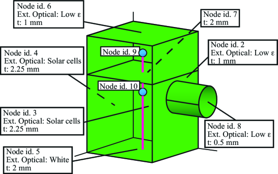
Figure 1: Satellite’s structure and node description. The front face, removed to see the interior, corresponds to node 1 and is equivalent to nodes 3 or 4.

To test the previously explained methods, we construct a small thermal model of a simple spacecraft, namely, a ten-node model of a Moon-orbiting satellite. Our satellite ten-node model supports a basic thermal structure and is simple enough for allowing one to explicitly display the main mathematical entities, e.g., the matrices $K$, $R$ and $J$. The satellite consists of a rectangular parallelepiped (a cuboid) of square base plus a small cylinder on one of its sides that simulates an observation instrument, as represented in Fig. 1. In addition, at a height of two thirds of the total height, there is an inner tray with the electronic equipment. The dimensions of the cuboid are $0.2\,\mathrm{m}\times 0.2\,\mathrm{m}\times 0.3\,\mathrm{m}$, and the cylinder has a length of 0.1 m and a radius of 0.04 m. The satellite’s frame is made of aluminum alloy, using plates 1 mm thick, except the bottom plate, which is 2 mm thick. This plate plays the role of a radiator and its outer surface is painted white to have high solar reflectance. The cylinder is made of the same aluminum alloy, as well as the tray; they are 0.5 mm and 2 mm thick, respectively. The sides of the satellite, except the one with the instrument, are covered with solar cells, which increase the sides’ thickness to 2.25 mm.

The thermal model of the satellite assigns one node to each face of the cuboid, one more to the cylinder and another to the tray, that is, eight nodes altogether. Furthermore, to conveniently split the total heat capacitance of the electronic equipment, it is convenient to add two extra nodes with (large) heat capacitance but with no surface that could exchange heat by radiation. Nodes of this type are called “non-geometrical nodes”. In the present case, they represent two boxes with equipment placed above and below the tray, respectively. We order the ten nodes as shown in Fig. 1. The lower box (node 10) is connected to the radiator by a thermal strap. Given the satellite’s structure and assuming appropriate values of the specific heat capacities, it is possible to compute the capacitances $C_{i},\;i=1\ldots,10,$ with the result given in Table 1. Using the value of the aluminum-alloy heat conductivity and assuming perfect contact between plates, we compute the conduction coupling constants $K_{ij}$ between nodes $i,j=1,\ldots,8$. The remaining conduction coupling constants are given reasonable values, shown in Eq. (39). The computation of the radiation coupling constants $R_{ij},\;i,j=1,\ldots,8,$ and $R_{i},\;i=1,\ldots,8,$ and indeed the computation of the external radiation heat inputs requires a detailed radiative model of the satellite, consisting of the geometrical view factors and the detailed thermo-optical properties of all surfaces. This radiative model allows us to compute the respective absorption factors Kreith .

Node	$C_{i}$ (J/K)	$\langle{\dot{Q_{i}}}\rangle$ (W)	$\widetilde{T}_{i}$ (${}^{\circ}\mathrm{C}$)
1	331.7	15.18	2.6
2	147.4	2.30	3.6
3	331.7	15.17	2.6
4	331.7	14.80	2.3
5	196.6	3.91	0.2
6	98.3	0.63	2.2
7	196.6	0aa	6.3
8	31.9	1.70	4.7
9	800.0	4.35	15.9
10	1400.0	6.15	11.1

Table 1: Node capacities and mean heat inputs with their associated steady-state temperatures.

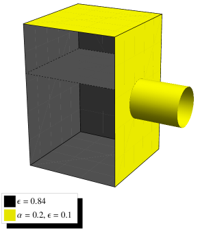
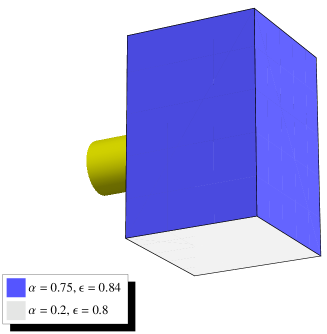
Figure 2: Thermo-optical properties of the satellite’s surfaces (details are given in the text).

The thermo-optical properties of the surfaces are assumed to be as realistic as possible, given the simplicity of the thermal model. All radiation reflection is assumed to be diffuse, as is common for many types of surfaces. The inner surfaces are painted black and have high emissivity, $\varepsilon=0.84$, to favor the uniformization of the interior temperature. The outer surfaces are of three types. The three sides covered with solar cells also have high emissivity, $\varepsilon=0.84$, to favor the cooling of the solar cells. On the other hand, they have high solar absorptivity, $\alpha_{\mathrm{s}}=0.75$. Of this 0.75, 0.18 is processed into electricity and the remaining 0.57 dissipates as heat in the solar cells. The top surface, the surface with the cylinder, and the cylinder itself (its two sides) have low emissivity, $\varepsilon=0.1$, and low solar absorptivity, $\alpha_{\mathrm{s}}=0.2$, which are chosen to simulate the effect of a multilayer insulator. In contrast, the bottom surface simulates a radiator, with $\varepsilon=0.8$ and $\alpha_{\mathrm{s}}=0.2$ (like an optical solar reflector). All of these thermo-optical properties are summarized in Fig. 2. For the computation of the corresponding absorption factors, we employ the ray-tracing Monte-Carlo simulation method provided by ESARAD^TM (ESATAN^TM’s radiation module) ESATAN .

Taking into account the above information, one obtains the following conduction (in W/K) and radiation (in W/K⁴) matrices:

$$(K_{ij}) = \frac{1}{10}\left(\begin{array}[]{cccccccccc}0&3.47&0&5.64&2.86&2.00&4.50&0&0&0\\ 3.47&0&3.47&0&1.67&1.33&3.50&3.00&0&0\\ 0&3.47&0&5.64&2.86&2.00&4.50&0&0&0\\ 5.64&0&5.64&0&2.86&2.00&4.50&0&0&0\\ 2.86&1.67&2.86&2.86&0&0&0&0&0&3.00\\ 2.00&1.33&2.00&2.00&0&0&0&0&0&0\\ 4.50&3.50&4.50&4.50&0&0&0&0&4.50&6.00\\ 0&3.00&0&0&0&0&0&0&0&0\\ 0&0&0&0&0&0&4.50&0&0&0\\ 0&0&0&0&3.00&0&6.00&0&0&0\end{array}\right),$$ (39)

$$(R_{ij}) = 10^{-10}\left(\begin{array}[]{cccccccccc}0&5.06&4.63&5.05&3.68&2.71&6.39&0&0&0\\ 5.06&0&5.05&4.63&3.68&2.70&6.39&0.13&0&0\\ 4.63&5.05&0&5.06&3.69&2.71&6.39&0&0&0\\ 5.05&4.63&5.06&0&3.69&2.70&6.38&0&0&0\\ 3.68&3.68&3.69&3.69&0&0&3.57&0&0&0\\ 2.71&2.70&2.71&2.70&0&0&7.19&0&0&0\\ 6.39&6.39&6.39&6.38&3.57&7.19&0&0&0&0\\ 0&0.13&0&0&0&0&0&0&0&0\\ 0&0&0&0&0&0&0&0&0&0\\ 0&0&0&0&0&0&0&0&0&0\end{array}\right),$$ (50)

$$(R_{i}) = 10^{-9}\,(2.86,0.32,2.86,2.86,1.81,0.23,0,0.23,0,0).$$ (51)

The satellite’s thermal characteristics are defined by the data set $\{C_{i},K_{ij},R_{ij},R_{i}\},$ but the radiation heat exchange depends on the nodal temperatures, which in turn depend on the heat input. As explained in Sect. II.1, the appropriate set of nodal temperatures corresponds to the steady-state for averaged heat inputs, given by the algebraic equation that results from making $\dot{T}_{(0)i}=0$ in Eq. (4). Since we need the external heat inputs and, therefore, the orbit, we proceed to define the orbit characteristics.

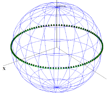
Figure 3: The 111 positions of the satellite in its orbit. The sunlight comes along the $x$ axis.

We choose a circular equatorial orbit $26\hskip 1.0pt926$ m above the Moon’s surface, such that ${\cal T}=6660$ s. The radiation heat input to the satellite consists, on the one hand, of the solar irradiation and the Moon’s albedo, and, on the other hand, of the Moon’s constant IR radiation. We take 0.12 for the mean Moon’s albedo and 270 K for the black-body equivalent temperature of the Moon. There is also heat produced by the dissipation of electrical power in the equipment (nodes 9 and 10). For the sake of simplicity, the dissipation rate is assumed to be constant, equal to the mean electrical power generated in an orbit. In a part of the orbit, the Moon eclipses the Sun, so the satellite receives no direct sunlight or albedo, although there is always IR radiation from the Moon. The satellite is stabilized such that the cylinder (the “observation instrument”) always points to the Moon and the longer edges are perpendicular to the orbit. The radiation heat input can be computed by taking into account the given orbital characteristics and the satellite’s thermo-optical characteristics, in particular, the absorption factors. It has been computed with ESARAD^TM, taking 111 positions on the orbit, that is, at intervals of one minute.

In Fig. 3, all 111 positions are plotted. The initial position of the satellite is at the subsolar point and it moves towards the east. The total external radiation heat input to the first eight nodes (the ones that receive radiation) is plotted in Fig. 4 (only at every other position, for clarity). Note the symmetry between nodes 1 and 3, which denote the lateral faces, covered with solar cells. Node 4 corresponds to the back side, also covered with solar cells. So the external radiation load on it has a similar time variation, but it is displaced. The solar radiation absorbed by all solar cells results in an orbital mean power rate of 10.5 W, dissipated in the equipment and split between nodes 9 and 10, which receive 4.35 and 6.15 W, respectively. The external radiation absorbed by the side with the cylinder (node 2) is considerably smaller than the radiation absorbed by the sides with solar cells, due to the low value of $\alpha_{\mathrm{s}}$ (and of $\varepsilon$, as well) for the corresponding surface. The bottom and top outer surfaces, which belong to nodes 5 and 6, respectively, have view factors for the external radiation that are much less favorable than those of the side surfaces. Nevertheless, the amount of lunar IR radiation absorbed by the bottom surface, due to its high $\varepsilon$, is such that the orbital mean of the external heat input to node 5 is, in fact, larger than the one for node 2 (see Table 1). Naturally, node 7, with no outer surfaces, does not absorb any external radiation.

\psfrag{heatinput}{{$\dot{Q}_{i}$ (W)}}\psfrag{nodes1to4}{{}}\psfrag{nodes5to8}{{}}\psfrag{t}{{$t$}}\includegraphics[width=227.62204pt]{h-in_1-4_b.eps}

(a) nodes 1–4

\psfrag{heatinput}{{$\dot{Q}_{i}$ (W)}}\psfrag{nodes1to4}{{}}\psfrag{nodes5to8}{{}}\psfrag{t}{{$t$}}\includegraphics[width=227.62204pt]{h-in_5-8_b.eps}

(b) nodes 5–8

Figure 4: Variation of the external heat input with time $t$ (in minutes) along the orbit. For both plots, the node numbers are denoted by shape, in the order: dots (1,5), squares (2,6), diamonds (3,7), and triangles (4,8).

To determine the hot and cold cases of the orbit, we compute the total heat load on the satellite for each position in the orbit, finding a maximum of 90.59 W at position 14 and a minimum of 18.65 W at any position in the eclipse, during which all the heat loads stay constant. The solution of the corresponding steady-state problems at position 14 and at a position in the eclipse yields the two sets of nodal temperatures (for the given node order):

Hot

$\{29.0,35.5,41.2,38.5,30.2,35.1,39.1,35.0,48.7,42.9\}\;^{\circ}\mathrm{C}$.

Cold

$\{-46.8,-45.0,-46.8,-49.1,-45.7,-47.1,-42.8,-44.1,-33.2,-37.0\}\;^{\circ}\mathrm{C}$.

The results in Sect. IV.1 show that the periodic thermal state does not reach these extreme temperatures, which could endanger the performance of the satellite.

IV.1 Jacobian matrix and periodic solution

We compute the averages $\langle{\dot{Q_{i}}}\rangle$ and substitute for them and the data set $\{K_{ij},R_{ij},R_{i}\}$ in Eq. (4) to find the steady state temperatures. The results are given in Table 1. Then, according to Eqs. (6) and (7), the Jacobian matrix is (in s^-1)

$${J=10^{-3}\left(\begin{array}[]{cccccccccc}-6.99&1.18&0.12&1.83&0.95&0.67&1.52&0&0&0\\ 2.64&-12.93&2.64&0.26&1.33&1.06&2.75&2.04&0&0\\ 0.12&1.17&-6.99&1.83&0.95&0.67&1.52&0&0&0\\ 1.83&0.12&1.83&-7.64&0.95&0.67&1.52&0&0&0\\ 1.61&1.01&1.61&1.61&-8.26&0&0.16&0&0&1.53\\ 2.27&1.59&2.27&2.27&0&-9.20&0.64&0&0&0\\ 2.56&2.06&2.56&2.56&0.15&0.31&-15.60&0&2.29&3.05\\ 0&9.43&0&0&0&0&0&-10.05&0&0\\ 0&0&0&0&0&0&0.56&0&-0.56&0\\ 0&0&0&0&0.21&0&0.43&0&0&-0.64\end{array}\right).}$$

By inspection, one can check that it has nonnegative off-diagonal and negative diagonal elements, that is to say, $-J$ is a $Z$-matrix. It is also diagonally dominant, namely, $|J_{ii}|\geq\sum_{j\neq i}|J_{ij}|$. The eigenvalues of $J$ are

$$-10^{-4}\{182.20,154.30,103.40,98.03,86.12,71.09,71.04,14.90,5.70,1.72\}.$$

Their inverses (in absolute value) give us the typical relaxation times of the corresponding thermal modes. Thus, we deduce that relaxation time of the fastest mode is about 55 s, whereas the relaxation time of the slowest one is $5\hskip 1.0pt813$ s. The latter time is similar to ${\cal T}=6\hskip 1.0pt660$ s.

The eigenvalues are real numbers and, furthermore, $J$ is diagonalizable, because the eigenvalues are different. Both properties also follow from $C^{1/2}JC^{-1/2}$ being almost symmetric: its antisymmetric part, $\delta A=(C^{1/2}JC^{-1/2}-C^{-1/2}J^{t}C^{1/2})/2$, is relatively small, namely, $\|\delta A\|/\|C^{1/2}JC^{-1/2}\|<10^{-3}$, where the matrix norm is the Frobenius norm (other standard matrix norms yield similar values). Therefore, the notion of “radiation conductance” (Sect. II.2) is appropriate in this case, as concerns its use in the linear equations. The thermal modes are almost normal, namely, the eigenvector matrix $P$ is such that $P^{t}CP=I$ with an error $<0.002.$ The most interesting eigenvector of $J$ is, of course, the positive (Perron) eigenvector, which corresponds to the slowest mode. The normalized positive eigenvector is

$$(0.259,0.276,0.259,0.257,0.275,0.267,0.327,0.264,0.471,0.423)~{}\mathrm{K}.$$

Note that the temperature increments are of a similar magnitude, except the ones of node 7 and, especially, nodes 9 and 10, which are associated, respectively, for the tray and the boxes of electronic equipment. The next mode, corresponding to the eigenvalue $-5.70\cdot 10^{-4}$, has one negative component (the ninth), and the remaining modes have more than one.

To calculate ${T}_{(1)}^{\infty}(t)$, we choose the Fourier series of Eq. (27) or, rather, the inverse discrete Fourier transform of Eq. (28), which can be computed with a FFT algorithm. The Fourier coefficients $\hat{F}(m)$ can also be computed with the FFT, according to Eq. (26). Once the vector ${T}_{(1)}^{\infty}$ at the 111 positions is available, the set of nodal temperatures corresponding to the first-order perturbative solution is ${T}_{i}^{\infty}(t)=\widetilde{T}_{i}+{T}^{\infty}_{(1)i}(t),\,i=1,\ldots,10,$ plotted in Fig. 5. A measure of the accuracy of this perturbative calculation is given by the second-order calculation in the next section. The truncation of the Fourier series imposed by the sampling of $F$ also is a source of error, unrelated to perturbation theory. The piecewise smoothness of the function ${T}_{(1)}^{\infty}(t)$ suggests that the error is small (but see Sect. IV.2).

\psfrag{heatinput}{{$\dot{Q}_{i}$ (W)}}\psfrag{nodes1to4}{{}}\psfrag{nodes5to8}{{}}\psfrag{t}{{$t$}}\psfrag{Tempcent}{{${T}_{i}^{\infty}$ (${}^{\circ}\mathrm{C}$)}}\psfrag{nodes1to5}{{}}\psfrag{nodes6to10}{{}}\includegraphics[width=227.62204pt]{T_1-5_b.eps}

(a) nodes 1–5

\psfrag{heatinput}{{$\dot{Q}_{i}$ (W)}}\psfrag{nodes1to4}{{}}\psfrag{nodes5to8}{{}}\psfrag{t}{{$t$}}\psfrag{Tempcent}{{${T}_{i}^{\infty}$ (${}^{\circ}\mathrm{C}$)}}\psfrag{nodes1to5}{{}}\psfrag{nodes6to10}{{}}\includegraphics[width=227.62204pt]{T_6-10_b.eps}

(b) nodes 6–10

Figure 5: Variation of the ten nodal temperatures with time $t$ (in minutes). For both plots, the node order is: dots (1,6), squares (2,7), diamonds (3,8), upward triangles (4,9), and downward triangles (5,10).

It is also interesting to see if the first-order perturbative calculation is affected by neglecting the fastest modes: according to the analysis at the end of Sect. II.1, these modes are expected to contribute in proportion to their relaxation times. The fastest mode relaxes in about 55 s, a short but non-negligible time. As a consequence, its contribution to ${T}_{(1)}^{\infty}$, which we find to have a maximum magnitude of 0.8 K, is small but non-negligible. But we can deduce that still faster modes, which would appear in a thermal model of the satellite with more nodes, are hardly necessary.

From the engineering standpoint, note that this satellite thermal model is successful, insofar as it predicts that all nodal temperatures stay within adequate ranges. In particular, nodes 9 and 10, corresponding to the boxes with electronic equipment, stay within the range from $4$ to 23 ${}^{\circ}\mathrm{C}$. These nodes are inner nodes with large thermal capacity and, hence, are protected against the larger changes in the external heat inputs. In contrast, the outer nodes are very exposed and undergo considerable variation in temperature, with especially sharp changes at the beginning and end of the eclipse.

IV.1.1 Second-order correction

\psfrag{heatinput}{{$\dot{Q}_{i}$ (W)}}\psfrag{nodes1to4}{{}}\psfrag{nodes5to8}{{}}\psfrag{t}{{$t$}}\psfrag{Tempcent}{{${T}_{i}^{\infty}$ (${}^{\circ}\mathrm{C}$)}}\psfrag{nodes1to5}{{}}\psfrag{nodes6to10}{{}}\psfrag{Temp}{{${T}_{(2)i}^{\infty}$ (K)}}\includegraphics[width=227.62204pt]{T2_1-5_b.eps}

(a) nodes 1–5

\psfrag{heatinput}{{$\dot{Q}_{i}$ (W)}}\psfrag{nodes1to4}{{}}\psfrag{nodes5to8}{{}}\psfrag{t}{{$t$}}\psfrag{Tempcent}{{${T}_{i}^{\infty}$ (${}^{\circ}\mathrm{C}$)}}\psfrag{nodes1to5}{{}}\psfrag{nodes6to10}{{}}\psfrag{Temp}{{${T}_{(2)i}^{\infty}$ (K)}}\includegraphics[width=227.62204pt]{T2_6-10_b.eps}

(b) nodes 6–10

Figure 6: Second-order correction to the temperatures (same node order as in Fig. 5).

According to Sect. II.1.1, the second-order perturbative correction ${T}_{(2)}^{\infty}$ to the periodic stationary solution is obtained by the same procedure as that for ${T}_{(1)}^{\infty}\,,$ but using a different driving function $G$ that is computed from $\widetilde{T}$ and from ${T}^{\infty}_{(1)}$ itself. The computations are straightforward and they yield the correction plotted in Fig. 6. This correction is always negative, because the negative term in the expression for $G$, Eq. (13), dominates over the positive term. The equation (10) for ${T}_{(1)}^{\infty}$ and the corresponding equation for ${T}_{(2)}^{\infty}$ are both linear, so ${T}_{(1)}^{\infty}$ and ${T}_{(2)}^{\infty}$ are proportional to the respective driving functions; and we can compare their magnitudes by comparing those driving functions, say, comparing typical values of $\dot{Q}$ and $6R_{i}\widetilde{T}_{i}^{2}\,{T_{(1)i}^{\infty}}^{2}$. This latter quantity can be roughly estimated as $6\cdot 2\cdot 10^{-9}\cdot 300^{2}\cdot 20^{2}$ W $\simeq 0.4$ W, whereas $\dot{Q}\simeq 10$ W (Table 1). Their ratio is about 25, which roughly agrees with the ratio of ${T}_{(1)}^{\infty}$ to ${T}_{(2)}^{\infty}$, as can be seen by comparing Fig. 5 to Fig. 6.

The order of magnitude of the second-order correction suggests that higher orders are not necessary, as we show next.

IV.2 Direct integration of the nonlinear equations

Of course, the periodic solution $T^{\infty}(t)$ can also be obtained by direct integration of the nonlinear Eqs. (1) with an adequate solver, based on Runge-Kutta or other methods Kris3 . Since the nonlinear analysis proves that the solution of Eqs. (1) will converge to the stationary periodic solution NoDy1 , the numerical solver must be run until this periodicity is established. Periodicity can be enforced by comparing the nodal temperatures at the beginning and the end of every period and demanding that they be equal, within some tolerance. To do this, ESATAN^TM provides the routine SOLCYC ESATAN . We have employed this routine to obtain the nonlinear equations’ cyclic solution (which is established in 10 periods if the tolerance is set to 0.001).

\psfrag{heatinput}{{$\dot{Q}_{i}$ (W)}}\psfrag{nodes1to4}{{}}\psfrag{nodes5to8}{{}}\psfrag{t}{{$t$}}\psfrag{Tempcent}{{${T}_{i}^{\infty}$ (${}^{\circ}\mathrm{C}$)}}\psfrag{nodes1to5}{{}}\psfrag{nodes6to10}{{}}\psfrag{Temp}{{${T}_{(2)i}^{\infty}$ (K)}}\psfrag{Tdiff}{{$\Delta{T}_{i}$ (K)}}\psfrag{nodes1and3and8}{{nodes 1, 3 and 8}}\includegraphics[width=227.62204pt]{Tdiff_1-3-8.eps}

Figure 7: The error in the temperature computed up to the second order. Only showing nodes 1 (dots), 3 (squares), and 8 (diamonds), which give rise to the largest errors.

To compare the cyclic solution obtained by the linear method with the “exact” solution $T^{\infty}(t)$ obtained by SOLCYC, we quantify the deviation by the vector of “errors”

$$\Delta{T}(t)=T^{\infty}(t)-\left[\widetilde{T}+{T}_{(1)}^{\infty}(t)+{T}_{(2)}^{\infty}(t)\right].$$

The largest components of $\Delta{T}$ are plotted in Fig. 7 (the remaining components stay in the range $[-0.1,0.1]\,^{\circ}\mathrm{C}$). There seem to be two branches for each node, but, in fact, it is an effect produced by the high-frequency oscillations of each $\Delta{T}_{i}(t)$. Notice that the error is generally small when compared with ${T}_{(2)}^{\infty}(t)$; namely, $|\Delta{T}(t)|\ll|{T}_{(2)}^{\infty}(t)|$ for each $t=k{\cal T}/n,\;k=0,\ldots,n-1$, except near the two positions corresponding to the beginning and end of the eclipse, where the heat inputs have discontinuities (Fig. 4). These discontinuities induce oscillations of certain amplitude about the true values of $T^{\infty}(t)$, due to the Gibbs phenomenon in the discrete Fourier transform (Sect. III). To suppress the oscillations, we would need a specific method for treating the Gibbs phenomenon; for example, we could use a smoother method for Fourier series summation, such as Cesàro summation Fourier

V Scalability and complexity of the linear method

The ten-node model studied in Sect. IV is too small to pose a computational problem, whether we employ the linear method or directly integrate nonlinear Eqs. (1). To assess the practical applicability of the linear method, we must study how it scales to realistic sizes and then compare it with the direct integration of Eqs. (1). Naturally, the first step in the method is to compute the steady-state temperature $\widetilde{T}_{i}\,,$ but this computation, arguably, is not a substantial part of the whole process and we do not consider it (it may take, say, between a few percent and one fith of the whole process, depending on the circumstances). The size of an orbiting spacecraft thermal model can be scaled with respect to the number of nodes, $N$, or the number of different positions in the orbit, $n$. However, while realistic models must have many nodes, an $n$ of about one hundred can generally be suitable. Note, in particular, that the condition that $N\ll n$ in the ten-node model is likely to be reversed in realistic models. For these reasons, the scaling with respect to $N$ is more relevant.

For the moment, let us neglect any special feature of Eqs. (1), such as possible coefficient sparsity. Then, the computational complexity of numerically integrating those equations is of order $N^{2}k$, where $k$ is the number of time steps taken. On the other hand, the complexity of the numerical integration of linear Eqs. (5) is also of order $N^{2}k$ [excluding the computation of $J(t)$]. We can employ the explicit integral, Eq. (8), which can be calculated with the trapezoidal rule, for example, but this does not reduce the complexity of the computation. However, for the stationary solution, Eq. (10), its expression as an integral over a period ${\cal T}$ sets the number of time steps to $n$, which is advantageous if $n<k$, where $k$ now is the number of steps necessary for some initial temperatures to relax to the stationary solution. Since we have to evaluate the integral in Eq. (10) for several times $t$, it is preferable to use the FFT, as discussed in Sect. III, so that the total operation count is of order $N^{2}\,n\log n$.

However, we have not taken into account matrix operations of considerable complexity. For example, the discrete Fourier transform, Eq. (27), involves the inverse of an $N\times N$ matrix ($-J$ plus a multiple of the identity matrix), and the inversion of a matrix is generally a process of order $N^{3}$ Num_rec . If we have to employ a process of order $N^{3}$, we may as well diagonalize $J$, because the diagonalization of a matrix also is generally a process of order $N^{3}$ Num_rec and the diagonalization of $J$ has several uses. Let us assume that we carry out this diagonalization and determine the independent thermal modes, which can then be employed to express Eq. (10) as Eq. (11) or to simplify the matrix operations in Eq. (27). If we roughly compare the computational complexity of order $N^{3}$ with the numerical integration complexity of order $N^{2}k$, we deduce that the diagonalization is worthwhile when $N<k$. Using the above estimate $n\sim 100$ and taking as relaxation time $k\sim 5n$ (the rough value for the ten-node model), we deduce that the determination of thermal modes can be useful just as a computational procedure for models with a few hundred nodes.

Let us now consider that $J$ is surely a sparse matrix, so iterative matrix methods can take advantage of this characteristic. In fact, there are two degrees of sparsity in $J$, associated with conduction or radiation coupling terms. The conductance matrix $K$ has to be very sparse, because conduction is a local process, so each node can only be coupled to a few nodes. In contrast, radiation is a nonlocal process and couples any pair of nodes that has a nonvanishing view factor. In addition to the different sparsity of conduction and radiation coupling matrices, there are two other circumstances that make them different: (i) we are assuming that the conductive coupling matrix just depends on material properties, so it is independent of the reference temperatures $\widetilde{T}_{i}$; (ii) the conduction coupling terms are significantly larger than the radiation coupling terms for the natural values of those temperatures. All of this suggests separating the conduction and radiation parts of $J$, and then diagonalizing the conduction part.

Based on the study in Sect. II.2, the diagonalization of the conduction part of $J$ boils down to the diagonalization of the (generalized) Laplacian matrix $-C^{-1/2}KC^{-1/2},$ and this matrix is sparse. Suitable iterative algorithms to perform this diagonalization are, for example, the Lanczos Gol-Van or the Davidson David algorithms. These algorithms are particularly useful when only a few of the largest or smallest eigenvalues are needed. This is indeed our case, as only the slower modes are expected to contribute to ${T}_{(1)}^{\infty}$ and ${T}_{(2)}^{\infty}\,.$ Once the conduction part of $J$ has been diagonalized, in the sense that the lowest eigenvalues and eigenvectors of the corresponding Laplacian matrix are known, the radiation part of $J$ can be treated as a perturbation, using matrix perturbation methods pert-methods ; Gol-Van .

Iterative matrix methods, combined with matrix perturbation methods or other methods, if necessary, can reduce the order $N^{3}$ to $N^{2}$ or even to almost linear and so allow us to diagonalize the Jacobians for the largest values of $N$ that appear in current thermal spacecraft models. Of course, the sparsity of thermal coupling matrices also facilitates the direct integration of the nonlinear Eqs. (1). However, their nonlinearity prevents one from taking advantage of the above mentioned approximations methods, for example, the reduction to the small subspace of slow modes, or the splitting into conduction and radiation in which the latter is treated as a matrix perturbation. Moreover, the linearization is useful in various respects. For example, the overall relaxation time, given by the eigenvalue of smallest magnitude, can be effectively bounded by inequalities ineq and some of these bounds can be found with little computational effort.

VI Summary and discussion

We have studied the evolution of the thermal state of an orbiting spacecraft and developed a linear approach to this problem that is based on a rigorous perturbative treatment of the exact nonlinear equations. The first-order perturbation equations, Eqs. (5), constitute the basic linear system, which can be applied to higher orders after calculating the corresponding driving terms. As the Jacobian matrix of the nonlinear equations has negative eigenvalues, the linear equations describe the relaxation to a stationary thermal state, namely, a periodic solution that is independent of the initial conditions and only depends on the external heat input. This relaxation is similar to the relaxation to steady-state under constant external heat load.

We have shown that the perturbative treatment reveals the scope of a common linearization procedure of a heuristic nature, in which the nonlinear equations are rendered linear by the definition of radiation conductances (Sect. II.2). If one previously calculates, with the correct nonlinear Eqs. (4), the reference steady-state condition that corresponds to the average external heat input, the deviation from that steady-state is well approximated by the linear equations with radiation conductances. The Jacobian matrix corresponding to radiation conductances, obtained in Eqs. (16) and (17), is related to a symmetric matrix and, therefore, is easier to diagonalize. Furthermore, this relation implies that the thermal modes are normal, like the vibrational modes of a mechanical system. Although the notion of radiation conductance is just an approximation, it serves nonetheless to show that the Jacobian matrix is diagonalizable and has real eigenvalues.

The diagonalization of the Jacobian matrix is useful for the computation of the stationary thermal state and also provides information on the relaxation to that state, because the relaxation times of the thermal modes are the inverses of the eigenvalues. These times span a considerable range, but the longest times are much more significant than the shortest times, because the latter depend on the details of the lumped-parameter thermal model employed whereas the former are essentially independent of it. In fact, a thermal model that has more nodes and therefore more details also has more thermal modes; but the slowest modes, which correspond to temperature changes in large parts of the spacecraft, are hardly affected by the details, whereas the fast modes can be significantly altered. The slowest mode, in particular, corresponds to a simultaneous but non-uniform increase (or decrease) of the temperature throughout the spacecraft and is hardly altered by small-scale changes.

The computation of the stationary thermal state with the linear method relies on an explicit integral, Eq. (10), or a Fourier expansion, Eq. (27). Given a sampling of the thermal driving function at equal time intervals, the periodic solution can be obtained through two discrete Fourier transforms: a direct transform to get the Fourier coefficients of the driving function and an inverse transform of the coefficient vector multiplied by a suitable matrix (Sect. III). Of course, the discrete Fourier transforms are best performed with a FFT algorithm. This computation is more efficient than the numerical computation of the integral, Eq. (10), if we need the values of the temperatures at all the given sampling times. However, the Fourier transform presents the Gibbs phenomenon, associated with sudden variations of the heat loads, as occur at eclipse times, for example. The Gibbs phenomenon introduces errors, but these errors could be suppressed with special methods.

The computation of the thermal modes and the stationary thermal state for a satellite ten-node thermal model confirms the validity of the linear method for a minimal but realistic model. The relaxation times span a considerable range, between 55 seconds and nearly one hundred minutes. Of course, the latter time must be almost independent of the particular thermal model used, whereas the former has no intrinsic significance, and, if the number of nodes grew, that time would shrink (thus further expanding the range of relaxation times). The slowest mode corresponds to node temperature increments with the same sign (positive by convention), whereas the increments corresponding to other modes have both signs. The periodic variation in the external heat input (Fig. 4) excites the thermal modes and produces a definite pattern of stationary temperature oscillations, well approximated by the first-order solution (Fig. 5). The second-order correction is small compared to the first-order solution, but it is worth computing, as it reaches 1.7 K. Higher order corrections are essentially negligible, but the error due to the Gibbs phenomenon at the eclipse positions reaches 0.6 K (at the most).

Focusing on the computational aspects of the linear approach, we have studied how it scales with the number $N$ of nodes and the number $n$ of sampling positions on the orbit. If the Jacobian matrix is dense, the complexity of the corresponding matrix operations is of order $N^{3}$. It is convenient to employ just one matrix operation, namely, the diagonalization of the Jacobian matrix, because then only a few of the slowest modes are needed for the remaining operations, so these have negligible complexity. The complexity of a direct numerical integration of the nonlinear equations is of order $N^{2}k$, $k$ being the number of time steps necessary for relaxation. For a low-altitude orbit, $k$ is expected to be on the order of one thousand, as for our Moon-orbiting satellite. Therefore, the linear method would be computationally effective as just an integration method only for models with a few hundred nodes. At any rate, the Jacobian matrix can be assumed to be sparse, and its conduction part can be assumed to be especially sparse, in addition to being the larger part of the Jacobian matrix and also being independent of the orbit. As the orbit may be subjected to changes in the planning of a mission, a convenient strategy probably is to diagonalize the conduction part at the outset and, when needed, add the radiation part within some approximation scheme. This strategy can be far more efficient than integrating the nonlinear equations each time.

Moreover, the strength of the linear approach lies with the insight that it provides about the thermal behavior of the spacecraft, as embodied by the decomposition of its thermal modes, of which only the slowest ones are significant. These significant modes can actually be obtained with a reduced thermal model using few nodes. Therefore, the linear approach is especially useful in the context of reduced models. Furthermore, it provides a method for model reduction based on the mode decomposition: this decomposition can be used to group nodes. Indeed, there is a technique for graph partitioning based on the eigenvalues and eigenvectors of the Laplacian matrix of the graph graph_eigenvec ; graph_part . According to Sect. II.2, this technique is applicable to the Jacobian matrix, but the details of this application are beyond the scope of the present paper and are left for future work.

Finally, our linear approach can surely be applied to other cyclic heating processes that involve radiation heat transfer.

Acknowledgments

We thank Isabel Pérez-Grande for bringing Ref. 13 to our attention.

References

F. Kreith, Radiation Heat Transfer for Spacecraft and Solar Power Plant Design. Intnal. Textbook Co., Scranton, Penn. (1962)

C.A. Wingate, Spacecraft Thermal Control. In: Fundamentals of Space Systems, V.L. Pisacane and R.G. Moore (eds.), Oxford Univ. Press (1994)

D.G. Gilmore (ed.), Spacecraft Thermal Control Handbook. The Aerospace Press, El Segundo (2002)

C.J. Savage, Thermal Control of Spacecraft. In: Spacecraft Systems Engineering, Third Edition, P. Fortescue, J. Stark and G. Swinerd (eds.), Wiley, Chichester (2003)

K. Oshima and Y. Oshima, An analytical approach to the thermal design of spacecrafts. Rep. No. 419, Inst. of Space and Aeronautical Science of Tokio (1968)

J.-R. Tsai, Overview of satellite thermal analytical model. Journal of Spacecraft and Rockets, 41, 120–125 (2004)

I. Pérez-Grande, A. Sanz-Andrés, C. Guerra and G. Alonso, Analytical study of the thermal behaviour and stability of a small satellite. Applied Thermal Engineering, 29, 2567–2573 (2009)

J. Gaite, A. Sanz-Andrés and I. Pérez-Grande, Nonlinear analysis of a simple model of temperature evolution in a satellite. Nonlinear Dynamics, 58, 405–415 (2009)

J. Gaite, Nonlinear analysis of spacecraft thermal models. Nonlinear Dynamics, 65, 283–300 (2011)

C.K. Krishnaprakas, Application of accelerated iterative methods for solution of thermal models of spacecraft. Journal of Spacecraft and Rockets, 32, 608–611 (1995)

C.K. Krishnaprakas, Efficient solution of spacecraft thermal models using preconditioned conjugate gradient methods. Journal of Spacecraft and Rockets, 35, 760–764 (1998)

M. Milman and W. Petrick, A note on the solution of a common thermal network problem encountered in heat-transfer analysis of spacecraft. Applied Mathematical Modelling, 24, 861–879 (2000)

C.K. Krishnaprakas, A comparison of ODE solution methods for spacecraft thermal problems. Heat Transfer Engineering, 19, 103–109 (1998)

ESATAN-TMS Thermal Engineering Manual and User Manual. Prepared by ITP Engines UK Ltd., Whetstone, Leicester, UK (2009)

A. Berman and R.J. Plemmons, Nonnegative Matrices in the Mathematical Sciences. Classics in Applied Mathematics, vol. 9, SIAM (1994)

E.J. Hinch, Perturbation methods, Cambridge Texts in Applied Mathematics (1991)

F.R.K. Chung, Spectral Graph Theory. Providence, RI: Amer. Math. Soc. (1997)

T. Biyikoglu, J. Leydold and P.F. Stadler, Laplacian Eigenvectors of Graphs: Perron-Frobenius and Faber-Krahn Type Theorems. Lecture Notes in Mathematics 1915, Springer (2007)

H.F. Davis, Fourier Series and Orthogonal Functions. Dover Publications (1989)

W.H. Press, S.A. Teukolsky, W.T. Vetterling, and B.P. Flannery, Numerical Recipes: The Art of Scientific Computing. Cambridge University Press, 3rd edition (2007)

G.H. Golub and C.F. Van Loan, Matrix Computations. The Johns Hopkins U. Press, Baltimore (1996)

M. Crouzeix, B. Philippe and M. Sadkane, The Davidson Method. SIAM Journal on Scientific Computing, 15, 62–76 (1994)

G.-X. Tian and T.-Z. Huang, Inequalities for the minimum eigenvalue of M-matrices. Electronic Journal of Linear Algebra, 28, 291–302 (2010)

U. Luxburg, A tutorial on spectral clustering. Statistics and Computing, 17, 395–416 (2007)