Toric cubes

Abstract

A toric cube is a subset of the standard cube defined by binomial inequalities. These basic semialgebraic sets are precisely the images of standard cubes under monomial maps. We study toric cubes from the perspective of topological combinatorics. Explicit decompositions as CW-complexes are constructed. Their open cells are interiors of toric cubes and their boundaries are subcomplexes. The motivating example of a toric cube is the edge-product space in phylogenetics, and our work generalizes results known for that space.

1 Introduction.

The standard $n$-dimensional cube $[0,1]^{n}$ is a commutative monoid under coordinatewise multiplication. In this article, we examine the natural class of submonoids of that monoid described next. A binomial inequality has the form

$$x_{1}^{u_{1}}x_{2}^{u_{2}}\cdots x_{n}^{u_{n}}\,\,\leq\,\,x_{1}^{v_{1}}x_{2}^{v_{2}}\cdots x_{n}^{v_{n}},$$ (1)

where the $u_{i}$ and $v_{j}$ are non-negative integers. A toric precube is a subset $\mathcal{C}$ of the cube $[0,1]^{n}$ that is defined by a finite collection of binomial inequalities. A toric cube $\mathcal{C}$ is toric precube that coincides with the closure of its strictly positive points. Equivalently, a toric cube is a subset $\mathcal{C}$ of the standard cube $[0,1]^{n}$ that is defined by binomial inequalities (1) and also satisfies $\,\mathcal{C}\,=\,\overline{\mathcal{C}\,\cap\,(0,1]^{n}}$. Example 3 illustrates the difference between a toric precube and a toric cube.

By definition, every toric cube is a basic closed semialgebraic set in $\mathbb{R}^{n}$. Thus, the present article can be regarded as a case study in real algebraic geometry BCR , with focus on a class of highly structured combinatorial objects.

Our first result is a parametric representation of toric cubes. We fix $n$ monomials ${\bf t}^{a_{1}},{\bf t}^{a_{2}},$ $\ldots,{\bf t}^{a_{n}}$ in $d$ unknowns $t_{1},t_{2},\ldots,t_{d}$. The representing map is a monoid homomorphism from the $d$-cube to the $n$-cube:

$$f\,:\,[0,1]^{d}\mapsto[0,1]^{n}\,,\,\,(t_{1},\ldots,t_{d})\mapsto({\bf t}^{a_{1}},{\bf t}^{a_{2}},\ldots,{\bf t}^{a_{n}}).$$ (2)

Our first result states that the image of any such monomial map of cubes is a toric cube and, conversely, all toric cubes admit such a parametrization:

Theorem 1.1

The toric cubes $\,\mathcal{C}$ in $[0,1]^{n}$ are precisely the images of other cubes $[0,1]^{d}$, for any positive integer $d$, under the monomial maps $f$ into $[0,1]^{n}$.

Example 1

Let $n=d=3$. The image of the monomial map

$$f\,:\,[0,1]^{3}\rightarrow[0,1]^{3}\,,\,\,(x,y,z)\mapsto(xy,yz,xz)=(a,b,c)$$

is the three-dimensional toric cube depicted in Figure 1. It consists of all points $(a,b,c)$ in $[0,1]^{3}$ that satisfy the three inequalities $a\geq bc,b\geq ac$ and $c\geq ab$.

The intersection of a toric cube with a coordinate subspace is homeomorphic to a convex polyhedral cone. This is seen by taking the logarithm of the positive coordinates. The collection of cells from these polyhedral cones glue together, but sometimes further refinements are required to avoid the situation in Example 3 when only a part of a boundary cell is glued onto a higher-dimensional open cell.

It is a problem of topological combinatorics to carry out these refinements in a systematic manner. The resolution of this problem is our second result:

Theorem 1.2

Every toric cube can be realized as a CW-complex whose open cells are interiors of toric cubes. This CW complex has the further property that the boundary of each open cell is a subcomplex.

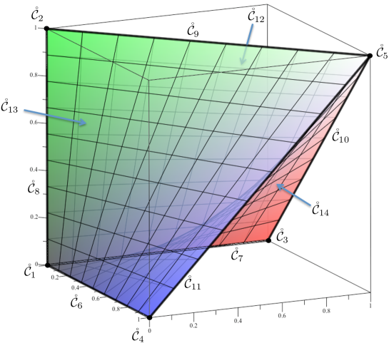
Figure 1: The toric cube in Example 1 with its CW cell decomposition as in Example 4.

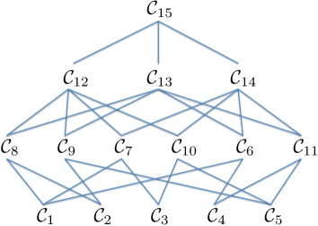
Figure 2: The face poset of the CW complex defined in Example 4 and drawn in Figure 1.

Our study of toric cubes is in part motivated by phylogenetics. In that context, the topological spaces studied by Kim Kim and Gill, Linusson, Moulton and Steel GLMS ; MS , are built from particularly well-behaved instances of toric cubes. The toric cube in Figure 1 is the smallest instance of this: it is the edge-product space of a tree with three leaves, as shown in (GLMS, , Figure 1). Note that we have redrawn the same poset in Figure 2 to indicate our cell labeling.

In those papers, every point of a toric cube corresponds to parameters of a statistical model that describe a phylogenetic tree. The observed data can be encoded as points in the standard cube from which the toric cube is realized. To infer the parameters of the model amounts to running a maximum likelihood algorithm to locate the point that in some sense is closest to the observed ones. Standard algorithms, such as Expectation-Maximization, behave badly on closed sets if the desired point is reached on the boundary. Thus, it is advantageous to break the space into open cells and restrict to the relevant pieces upon which one could get the algorithms to function well. For spaces where the points correspond to random models, there is often a first natural stratification by combinatorial type; in the case of phylogenetic trees, each open cell corresponds to a certain tree topology and the points in that cell describe the lengths of the branches. It may be speculated that our construction here may prove to be useful also for other models in algebraic statistics DSS .

Cellular complexes that are described only by their combinatorial incidence relations, like simplicial complexes, are called regular. Gill, Linusson, Moulton and Steel GLMS proved that the specific toric cubes arising in the above phylogenetic context are regular. In the first arXiv version of this paper, we conjectured that all complexes built from toric cubes share this property. Our conjecture was subsequently proved by Basu, Gabrielov and Vorobjov, using the theory of monotone semi-algebraic maps they had developed in BGV ; BGV2 . They established:

Theorem 1.3 (Basu, Gabrielov and Vorobjov, Section 6 of BGV2 )

Every toric cube is homeomorphic to a closed ball, and every CW-complex whose closed cells are toric cubes is regular. In particular, the CW-complexes for toric cubes constructed in the proof of Theorem  1.2 are regular.

2 Parametrization and Implicitization

Toric cubes are objects of real algebraic geometry that have a very nice combinatorial structure. In particular, they are basic semialgebraic sets, that is, they can be defined by conjunctions of polynomial inequalities.

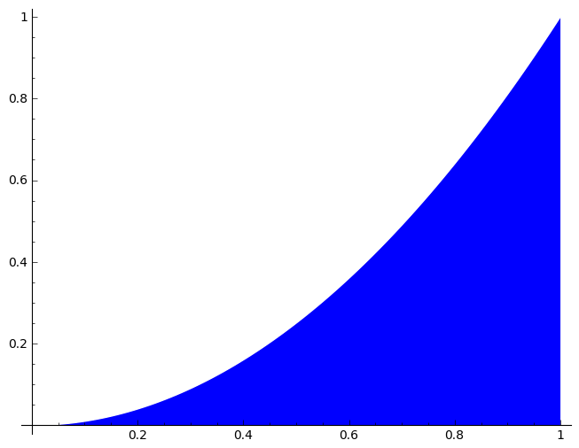
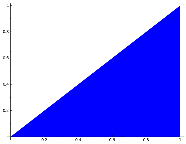
$(x,x^{2}y)$	$(x,xy^{2})$
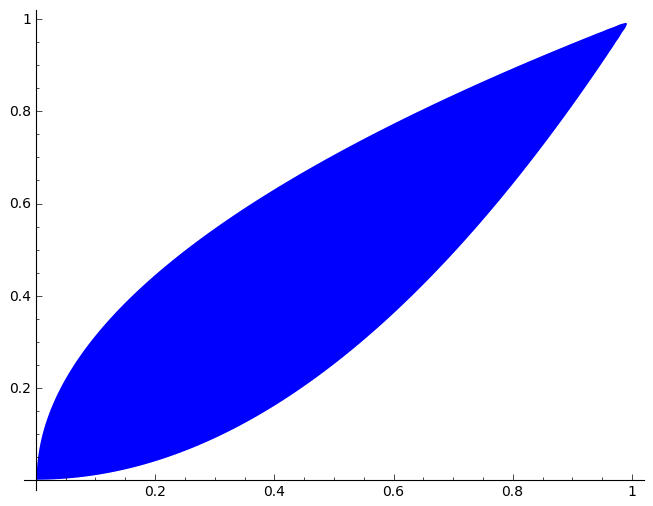
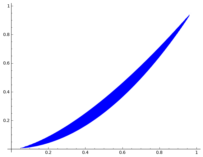
$(x^{2}y,xy^{2})$	$(x^{2}y,x^{3}y^{2})$

Figure 3: Parameterizations of two-dimensional toric cubes inside the square $[0,1]^{2}$.

We begin our discussion with an illustration of toric cubes in dimension $2$.

Example 2

Let $n=d=2$ and consider monomial self-maps of the square:

$$f\,:\,\,[0,1]^{2}\,\rightarrow\,[0,1]^{2}\,,\,\,\,(x,y)\,\mapsto\,(x^{i}y^{j},x^{k}y^{l}).$$

If $i,j,k,l>0$ then the toric cube $\mathcal{C}=f\bigl{(}[0,1]^{2}\bigr{)}$ is a region bounded by two monomial curves from $(0,0)$ to $(1,1)$. If precisely one of $i,j,k,l$ is zero then $\mathcal{C}$ will include two edges of $[0,1]^{2}$. Some specific instances are shown in Figure 3.

The image of the cube $[0,1]^{d}$ under an arbitrary polynomial map is always a semialgebraic set, that is, it can be defined by a Boolean combination of polynomial inequalities. This follows from Tarski’s Theorem on Quantifier Elimination (BCR, , §5.2). However, such a semialgebraic set is usually not basic: conjunctions do not suffice. For a concrete example, consider the map

$$[0,1]^{2}\rightarrow\mathbb{R}^{2},\,\,(x,y)\mapsto(x+y,x+2y^{2}-2y).$$

Its image in $\mathbb{R}^{2}$ is not a basic semialgebraic set since one edge of the square is mapped into the interior of the image, as seen in Figure 4.

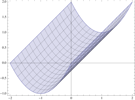
Figure 4: This image of the square is not basic in $\mathbb{R}^{2}$.

Our first result ensures that such a folding never occurs for monomial maps.

Proof (Theorem 1.1)

We first prove that monomial images of cubes are toric cubes. Let $\mathcal{C}$ denote the image in $[0,1]^{n}$ of the map $f$ in (2). Write $\mathcal{C}^{+}=\mathcal{C}\,\cap\,(0,1]^{n}$ for its subset of positive points. Then $\mathcal{C}^{+}$ is non-empty, and every point in $\mathcal{C}\backslash\mathcal{C}^{+}$ is the limit of a sequence of points in $\mathcal{C}^{+}$. Let ${\rm log}(\mathcal{C}^{+})$ denote the image of $\mathcal{C}^{+}$ in $\mathbb{R}^{n}$ under the coordinatewise logarithm map, with reversed signs. The cone ${\rm log}(\mathcal{C}^{+})$ is the image of the positive orthant $\,{\rm log}((0,1]^{d})=\mathbb{R}^{d}_{\geq 0}\,$ under the linear map $A:\mathbb{R}^{d}\rightarrow\mathbb{R}^{n}$, where $A$ is the matrix whose rows are the vectors ${\bf a}_{1},{\bf a}_{2},\ldots,{\bf a}_{n}$. In particular, ${\rm log}(\mathcal{C}^{+})$ is a convex polyhedral cone that is defined over $\mathbb{Q}$. By the Weyl-Minkowski Theorem Zie , we can write the cone ${\rm log}(\mathcal{C}^{+})$ as the solution set of a finite system of linear inequalities of the form

$$u_{1}x_{1}+u_{2}x_{2}+\cdots+u_{n}x_{n}\,\,\leq\,\,v_{1}x_{1}+v_{2}x_{2}+\cdots+v_{n}x_{n},$$ (3)

where the $u_{i}$ and $v_{j}$ are non-negative integers. By applying the exponential map, we conclude that $\mathcal{C}^{+}$ is defined, as a subset of $(0,1]^{n}$, by a finite set of binomial inequalities. Since $\mathcal{C}=\overline{\mathcal{C}^{+}}$, the result follows from Lemma 1 below.

For the converse, we can reverse the reasoning in the argument above. Suppose that $\mathcal{C}$ is a toric cube, so it is the closure of $\mathcal{C}^{+}=\mathcal{C}\,\cap\,(0,1]^{n}$. The cone ${\rm log}(\mathcal{C}^{+})$ is defined by the linear inequalities (3) corresponding to the binomial inequalities (1) that define $\mathcal{C}$. We can write this cone as the image of some positive orthant $\mathbb{R}^{d}_{\geq 0}$ under some linear map. That linear map is given by an integer matrix $A$ with $d$ columns and $n$ rows ${\bf a}_{1},{\bf a}_{2},\ldots,{\bf a}_{n}$. The image of $(0,1]^{d}$ under the corresponding monomial map $f$ equals $\mathcal{C}^{+}$, and hence the image of the closed cube $[0,1]^{d}$ under $f$ is $\mathcal{C}$. ∎

Lemma 1

Let $\mathcal{C}$ be a toric precube and $\mathcal{C}^{+}=\mathcal{C}\,\cap\,(0,1]^{n}$ its subset of points with positive coordinates. Then the closure $\overline{\mathcal{C}^{+}}$ is a toric cube.

Proof

Let $\mathcal{C}$ be a toric precube in $[0,1]^{n}$ that is defined by a system of $N$ binomial inequalities (1). We present an algorithm that creates a finite list of additional binomial inequalities such that the solution set of the new enlarged system equals $\overline{\mathcal{C}^{+}}$. Thus we give an algorithm for the cubification of a precube.

The procedure starts with the following step. For each of the $N$ given inequalities (1) we introduce a new variable $\epsilon_{i}$ and we consider the binomial

$$x_{1}^{u_{1}}x_{2}^{u_{2}}\cdots x_{n}^{u_{n}}\,\,-\,\,x_{1}^{v_{1}}x_{2}^{v_{2}}\cdots x_{n}^{v_{n}}\cdot\epsilon_{i}.$$

Thus, we now have a collection of $N$ binomials in $N+n$ variables. Let $I$ be the ideal in the polynomial ring generated by these binomials and compute its saturation $I^{\rm sat}$ with respect to all unknowns. We replace $I$ by the corresponding lattice ideal $I^{\rm sat}$. Algorithmically, this corresponds to computing a Markov basis, say, in the software 4ti2. For background on Markov bases see (DSS, , §1).

Since $I^{\rm sat}$ is a lattice ideal, the complex variety $V(I^{\rm sat})$ is a finite union of toric varieties. These components are all orbit closures of the same torus action, and only one of them intersects the positive orthant in $\mathbb{R}^{n+N}$. The corresponding toric ideal $I^{\rm tor}$ is a prime component of the radical ideal $I^{\rm sat}$. Now, the toric variety $V(I^{\rm tor})$ is the closure of its non-zero points. The same holds for the real points and the non-negative points in the toric variety:

$$V(I^{\rm tor})\,\cap\,[0,1]^{N+n}\,\,=\,\,\overline{V(I^{\rm tor})\,\cap\,(0,1]^{N+n}}.$$

The projection of this set onto the $n$ coordinates $x_{1},\ldots,x_{n}$ is precisely the set $\overline{\mathcal{C}^{+}}$. We obtain a system of binomial inequalities that defines $\overline{\mathcal{C}^{+}}$ from the generators $\,{\bf x}^{\bf u}\epsilon^{\bf b}-{\bf x}^{\bf v}\epsilon^{\bf c}\,$ of the toric ideal $I^{\rm tor}$. Namely, we take the inequality ${\bf x}^{\bf u}\leq{\bf x}^{\bf v}$ if ${\bf b}=0$ and ${\bf c}\not=0$, we take the inequality ${\bf x}^{\bf u}\geq{\bf x}^{\bf v}$ if ${\bf b}\not={\bf 0}$ and ${\bf c}={\bf 0}$, and we ignore the generator if both ${\bf b}$ and ${\bf c}$ are non-zero. The resulting finite system of binomial inequalities shows that $\overline{\mathcal{C}^{+}}$ is a toric cube. ∎

Example 3

Let $\mathcal{C}$ denote the toric precube in $[0,1]^{4}$ defined by the inequalities

$$ac\geq bd\quad\hbox{and}\quad bc\geq ad.$$

This precube is not a toric cube because it contains the entire face of points $(0,0,c,d)$ while every point in $\mathcal{C}^{+}$ satisfies $c\geq d$. The toric cube $\overline{\mathcal{C}^{+}}$ is cut out by the three inequalities $\,ac\geq bd$, $\,bc\geq ad$ and $c\geq d$. To compute a parametric representation of $\overline{\mathcal{C}^{+}}$, we take the negated logarithm and consider the cone

$$\{\,(A,B,C,D)\in\mathbb{R}_{\geq 0}^{4}\,:\,A+C\leq B+D,\,B+C\leq A+D\,\}.$$ (4)

This cone has the five extreme rays $(1,1,0,0),(1,0,0,1),(0,1,0,1),(0,0,1,1)$ and $(0,0,0,1)$. The $4\times 5$-matrix with these columns specifies the linear map $\,\mathbb{R}_{\geq 0}^{5}\rightarrow\mathbb{R}_{\geq 0}^{4}$ whose image is the cone (4). Writing the rows of that matrix as monomials, we obtain the desired parametrization of the toric cube $\overline{\mathcal{C}^{+}}$:

$$[0,1]^{5}\rightarrow[0,1]^{4}\,:\,(t_{1},t_{2},t_{3},t_{4},t_{5})\mapsto(t_{1}t_{2},t_{1}t_{3},t_{4},t_{2}t_{3}t_{4}t_{5})=(a,b,c,d).$$

3 Cell Decomposition

In this section we study toric cubes through the lens of topological combinatorics, and we prove Theorem 1.2. Our task is to decompose a given toric cube as a CW-complex whose open cells are interiors of toric cubes with the further property that the boundaries of these cells are subcomplexes. We begin with the following basic observation concerning the topology of toric cubes.

Remark 1

Every toric cube is contractible. This is seen from the monomial parametrization $f$ as in (2). Namely, the map $g(t_{1},\ldots,t_{d},s)=f(st_{1},\ldots,st_{d})$ gives a deformation retraction of the toric cube onto $\mathbf{0}$.

To build a CW-complex from toric cubes it is necessary to put toric cubes on the $0$-boundaries. To this end, monomial maps like $x\mapsto(x,0,0)$ are allowed. This is consistent with the previous definition after removing redundant zeros. The singleton $\{\mathbf{0}\}$ is considered to be a toric cube of dimension $0$. In this section toric cubes are mainly described by way of their monomial parametrizations.

The CW-complexes treated in this text are well-behaved, and we give a restricted definition that is suitable for our purposes. For more general versions see lundellWeingram . Let $D^{m}$ denote the closed $m$-dimensional disc, and let $\partial D^{m}=S^{m-1}$ denote its boundary. Its interior, denoted $\mathring{D}^{m}=D^{m}\backslash\partial D^{m}$, is an open $m$-cell.

Definition 1

An $m$-dimensional CW-complex is a topological subspace $X^{m}$ of $\mathbb{R}^{n}$ that is constructed recursively in the following way:

• If $m=0$ then $X^{0}$ is a discrete set of points.

• If $m>1$ then $X^{m}$ is given by the following data:

  • an $(m-1)$-dimensional CW-complex $X^{m-1}$ in $\mathbb{R}^{n};$

  • a partition $\coprod_{\alpha\in I}\sigma_{\alpha}^{m}$ of $\,X^{m}\backslash X^{m-1}\,$ into open $m$–cells;

  • for every index $\alpha\in I,$ there is a characteristic map $\Phi_{\alpha}:D^{m}\rightarrow X^{m}$ such that $\Phi_{\alpha}(\partial D^{m})\subseteq X^{m-1}$ and the restriction of $\Phi_{\alpha}$ to the open cell $\mathring{D}^{m}$ is a homeomorphism with image $\sigma_{\alpha}^{m}.$

One common way to identify a CW-complex for a space $X$ is to partition $X$ into open cells of different dimensions and to give characteristic maps for each cell in that partition. We demonstrate this for our running example.

Example 4

Consider the toric cube $\mathcal{C}$ given by the monomial map $f(x,y,z)=(xy,yz,xz)$ in Example 1. We define a CW-complex for $\mathcal{C}$ with $15$ cells by

$$\begin{array}[]{lll}f_{15}(x,y,z)=(xy,yz,xz),&\mathcal{C}_{15}=f_{15}([0,1]^{3}),&\mathring{\mathcal{C}}_{15}=f_{15}((0,1)^{3}),\\ f_{14}(x,y)=(x,y,xy),&\mathcal{C}_{14}=f_{14}([0,1]^{2}),&\mathring{\mathcal{C}}_{14}=f_{14}((0,1)^{2}),\\ f_{13}(x,y)=(x,xy,y),&\mathcal{C}_{13}=f_{13}([0,1]^{2}),&\mathring{\mathcal{C}}_{13}=f_{13}((0,1)^{2}),\\ f_{12}(x,y)=(xy,x,y),&\mathcal{C}_{12}=f_{12}([0,1]^{2}),&\mathring{\mathcal{C}}_{12}=f_{12}((0,1)^{2}),\\ f_{11}(x)=(1,x,x),&\mathcal{C}_{11}=f_{11}([0,1]),&\mathring{\mathcal{C}}_{11}=f_{11}((0,1)),\\ f_{10}(x)=(x,1,x),&\mathcal{C}_{10}=f_{10}([0,1]),&\mathring{\mathcal{C}}_{10}=f_{10}((0,1)),\\ f_{9}(x)=(x,x,1),&\mathcal{C}_{9}=f_{9}([0,1]),&\mathring{\mathcal{C}}_{9}=f_{9}((0,1)),\\ f_{8}(x)=(0,0,x),&\mathcal{C}_{8}=f_{8}([0,1]),&\mathring{\mathcal{C}}_{8}=f_{8}((0,1)),\\ f_{7}(x)=(0,x,0),&\mathcal{C}_{7}=f_{7}([0,1]),&\mathring{\mathcal{C}}_{7}=f_{7}((0,1)),\\ f_{6}(x)=(x,0,0),&\mathcal{C}_{6}=f_{6}([0,1]),&\mathring{\mathcal{C}}_{6}=f_{6}((0,1)),\\ &\mathcal{C}_{5}=\{(1,1,1)\},&\mathring{\mathcal{C}}_{5}=\{(1,1,1)\},\\ &\mathcal{C}_{4}=\{(1,0,0)\},&\mathring{\mathcal{C}}_{4}=\{(1,0,0)\},\\ &\mathcal{C}_{3}=\{(0,1,0)\},&\mathring{\mathcal{C}}_{3}=\{(0,1,0)\},\\ &\mathcal{C}_{2}=\{(0,0,1)\},&\mathring{\mathcal{C}}_{2}=\{(0,0,1)\},\\ &\mathcal{C}_{1}=\{(0,0,0)\},&\mathring{\mathcal{C}}_{1}=\{(0,0,0)\}.\\ \end{array}$$

Here, the open cells of the CW-complex are $\mathring{\mathcal{C}}_{1},\ldots,\mathring{\mathcal{C}}_{15}$ and the closed cells are $\mathcal{C}_{1},\ldots,\mathcal{C}_{15}.$ In Figure 1, the CW-complex is drawn with all open faces marked. The closed cells, ordered by containment, form the face poset in Figure 2. This poset is identical to the one seen in the phylogenetic application (GLMS, , Figure 1).

The existence of a CW complex for toric cubes can be derived from standard theory lundellWeingram . However, being combinatorialists, we seek to find a small explicit one, ideally with the properties described in the following remark:

Remark 2

If the image of every $\partial D^{n}$ in the construction of a CW-complex is an $(n-1)$–dimensional topological manifold (that is, if each point has a neighborhood homeomorphic to the Euclidean $(n-1)$–dimensional space), then the CW-complex can be encoded combinatorially as the colimit of a diagram of spaces on a poset graded by dimension. This strategy was used by van Kampen in his thesis for combinatorial descriptions of cell complexes, and is explained for CW-complexes in (lundellWeingram, , Chapter 3). If the morphisms in this diagram are homotopic to constant maps, then its homotopy colimit is the nerve, which, if described as a simplicial complex, is the order complex of the aforementioned poset. The simplest case of this is when the image of each $\partial D^{n}$ is homeomorphic to a sphere. Such a CW-complex is called regular.

In Example 4 the monomial map $f$ defining the toric cube and the characteristic map were the same. However, in general this will not be the case, e.g. when the dimension of the image drops relative to the domain. We typically need to subdivide. This will be explained in Example 5 and Proposition 1.

Before proceeding, we recall and introduce some notation. The map $\log:(0,1]^{d}\rightarrow[0,\infty)^{d}$ is defined coordinate-wise by the negated logarithm. This log map is a homeomorphism, and so is its inverse exp map. For a toric cube $\mathcal{C}$, its interior is best viewed in log-space. The closed polyhedral cone $\mathcal{D}=\log(\mathcal{C}\cap(0,1]^{d})$ is full-dimensional in some lineality space and its interior is $\mathring{\mathcal{D}}.$ The interior of the toric cube $\mathcal{C}$ is $\mathring{\mathcal{C}}=\exp(\mathring{\mathcal{D}}).$ The dimensions of $\mathcal{C},\mathring{\mathcal{C}},\mathcal{D}$ and $\mathring{\mathcal{D}}$ are all the same. For a zero-dimensional toric cube, set $\mathring{\mathcal{C}}=\mathcal{C}.$

Example 5

Let $d=4,n=3$ and consider the toric cube given by the map

$$f(t_{1},t_{2},t_{3},t_{4})\,\,\,=\,\,\,(t_{1}t_{2}t_{4},t_{2}t_{3},t_{3}t_{4}).$$

We want the interior of the image to be our only $3$-dimensional cell, but it is the image of an open $4$-cell under the monomial map $f$. We cannot use this map together with the $4$-dimensional cubical domain right off as a characteristic map since this map is not injective on the interior. The cone in log-space of this toric cube is spanned by the four rays

$$r_{1}=(1,0,0),\,\,r_{2}=(1,1,0),\,\,r_{3}=(0,1,1),\,\,r_{4}=(1,0,1).$$

A cross section of that cone is a quadrilateral with the vertices corresponding to the rays in that order. The face poset of that quadrilateral has nine elements, labeled $1,2,3,4,12,23,34,14$ and $1234$. To start constructing a characteristic map, we subdivide to get simplicial pieces. Our new rays will have the form $r_{\sigma}=\sum_{i\in\sigma}r_{i}.$ Considering the various $\sigma$ in the face poset $P$, we obtain:

$$\begin{array}[]{c}r_{\{1,2,3,4\}}=(3,2,2),\\ r_{\{1,2\}}=(2,1,0),\,r_{\{2,3\}}=(1,2,1),\,r_{\{3,4\}}=(1,1,2),\,r_{\{1,4\}}=(2,0,1),\\ r_{\{1\}}=(1,0,0),\,\,r_{\{2\}}=(1,1,0),\,\,r_{\{3\}}=(0,1,1),\,\,r_{\{4\}}=(1,0,1).\\ \end{array}$$ (5)

The rays corresponding to the maximal flags in $P$ span simplicial cones that subdivide the cone spanned by the initial four rays. The $3\times 9$-matrix with column vectors (5) defines a new monomial map $\,\mathrm{sd}(f):[0,1]^{P}\rightarrow[0,1]^{3}\,$ by

$$(t_{\{1\}},t_{\{2\}},t_{\{3\}},t_{\{4\}},t_{\{1,2\}},t_{\{2,3\}},t_{\{3,4\}},t_{\{1,4\}},t_{\{1,2,3,4\}})\quad\mapsto$$

$$\begin{array}[]{l}(\,t_{\{1\}}t_{\{2\}}t_{\{4\}}t_{\{1,2\}}^{2}t_{\{2,3\}}t_{\{3,4\}}t_{\{1,4\}}^{2}t_{\{1,2,3,4\}}^{3},\\ \,\,\,t_{\{2\}}t_{\{3\}}t_{\{1,2\}}t_{\{2,3\}}^{2}t_{\{3,4\}}t_{\{1,2,3,4\}}^{2},\,\,\,\,\,\,t_{\{3\}}t_{\{4\}}t_{\{2,3\}}t_{\{3,4\}}^{2}t_{\{1,4\}}t_{\{1,2,3,4\}}^{2}).\end{array}$$

By setting $\,t_{1}=t_{\{1\}}t_{\{1,2\}}t_{\{1,4\}}t_{\{1,2,3,4\}}$ and similarly for $t_{2},t_{3},t_{4}$, we see that $f$ and $\mathrm{sd}(f)$ have exactly the same image. Thus, they define the same toric cubic. Guided by the simplicial subdivision above, we define $D\subset[0,1]^{P}$ to be

From the subdivision we can derive that $\,\mathrm{sd}(f)(D)=\mathrm{sd}(f)([0,1]^{P})$ $=f([0,1]^{4}).$ The domain $D$ is $3$-dimensional, as is the toric cube, and one can see that the restriction of $\mathrm{sd}(f)$ to the relative interior of $D$ is a homeomorphism onto the interior of the toric cube, as required for the characteristic maps. What remains to be shown at this point is that $D$ is in fact a $3$-dimensional ball. This is true, and we present a general argument in the proof of the next proposition.

Proposition 1

Let $\mathcal{C}\subset[0,1]^{n}$ be a toric cube and consider the convex polytope

$$\mathcal{P}\,\,=\,\,\bigl{\{}\,\mathbf{y}\in\log(\mathcal{C}\cap(0,1]^{n})\mid\mathbf{y}\cdot\mathbf{1}\leq 1\bigr{\}}.$$

There exists a continuous map $\Phi:\mathcal{P}\rightarrow\mathcal{C}$ whose restriction to the interior of $\mathcal{P}$ is a homeomorphism onto the interior of $\mathcal{C}$, with the property that the restriction of $\Phi$ to the boundary of $\mathcal{P}$ maps onto the boundary of $\mathcal{C}.$

Proof

The cone $\mathcal{D}=\log(\mathcal{C}\cap(0,1]^{n})$ is spanned by some non-negative integer rays $r_{1},r_{2},\ldots,r_{d}$. The toric cube is the image of the monomial map $f(t_{1},t_{2},\ldots,t_{d})=(m_{1},m_{2},\ldots,m_{n})$ where $m_{j}=\prod_{i=1}^{d}t_{i}^{r_{i}\cdot e_{j}}$ and $e_{j}$ is the $j$th unit vector. Without loss of generality we may assume that $\,r_{1}\cdot\mathbf{1}=\cdots=r_{d}\cdot\mathbf{1}$.

The non-empty subsets $S$ of $\{1,2,\ldots,d\}$ such that $\{r_{i}\mid i\in S\}$ is a minimal set of spanning rays of a face of $\mathcal{D}$, ordered by inclusion, is a poset $P.$ This poset $P$ is isomorphic to the face poset of $\mathcal{D}$ minus the minimal element.

We fix rays $\,r_{\sigma}=\sum_{i\in\sigma}r_{i}\,$ for each $\sigma\in P$, and we define a monomial map $\,\mathrm{sd}(f):[0,1]^{P}\rightarrow[0,1]^{n}\,$ by sending $\,(t_{\alpha})_{\alpha\in P}\,$ to $\,(m_{1}^{\mathrm{sd}},m_{2}^{\mathrm{sd}},\ldots,m_{n}^{\mathrm{sd}})\,$ where

$$m_{j}^{\mathrm{sd}}\,\,=\,\,\prod_{\sigma\in P}t_{\sigma}^{\sum_{i\in\sigma}r_{i}\cdot e_{j}}.$$

The cone in log-space defined by $\mathrm{sd}(f)$ is the same as the one for $f,$ but we have introduced rays that barycentrically subdivide it. The simplicial cones in that subdivision are indexed by the set of maximal chains in $P$. We define

$$D\quad=\bigcup_{\hbox{$C$ maximal chain of $P$}}\quad\prod_{\sigma\in P}\quad\left\{\begin{array}[]{cl}\,[0,1]&\quad{\rm if}\,\,\sigma\in C,\\ \,\{1\}&\quad{\rm if}\,\,\sigma\not\in C.\end{array}\right.$$

The barycentric subdivision ensures that $\mathcal{C}=f([0,1]^{d})=\mathrm{sd}(f)(D)$. Moreover, the restriction of $\mathrm{sd}(f)$ to the interior of $D$ is a homeomorphism onto $\mathring{\mathcal{C}}$.

We now construct a homeomorphism between $D$ and the polytope. We first fix the antipodal map, componentwise defined by $t\rightarrow 1-t,$ to get a homeomorphism $a:D^{\prime}\rightarrow D$ for

$$D^{\prime}\quad=\bigcup_{\hbox{$C$ maximal chain of $P$}}\quad\prod_{\sigma\in P}\quad\left\{\begin{array}[]{cl}\,[0,1]&\quad{\rm if}\,\,\sigma\in C,\\ \,\{0\}&\quad{\rm if}\,\,\sigma\not\in C.\end{array}\right.$$

Let $\Delta$ be the simplex in $\mathbb{R}^{P}$ spanned by the unit vectors and the origin. There is a standard homeomorphism from $\Delta$ to $[0,1]^{P}$ which maps $\,\mathbf{t}=(t_{\sigma})_{\sigma\in P}\neq\mathbf{0}\,$ to $\,\frac{\sum_{\sigma\in P}t_{\sigma}}{\max_{\sigma\in P}t_{\sigma}}\mathbf{t}\,$ and $\mathbf{0}$ to $\mathbf{0}$. Restricting this map to get the image $D^{\prime}$, we obtain a homeomorphism $b:D^{\prime\prime}\rightarrow D^{\prime}$ for $D^{\prime\prime}$ as follows.

By construction, $D^{\prime\prime}$ is the cone with apex $\mathbf{0}$ over the standard realization of the order complex of the poset $P$. Since $P$ is the face poset (minus the minimal element) of the polyhedral cone $\mathcal{D}$, we have a homeomorphism $c$ from the polytope $\{\mathbf{y}\in\mathcal{D}\mid\mathbf{y}\cdot\mathbf{1}\leq 1\}=\{\mathbf{y}\in\log(\mathcal{C}\cap(0,1]^{n})\mid\mathbf{y}\cdot\mathbf{1}\leq 1\}$ to $D^{\prime\prime}$. The composition of these maps gives a map $\Phi$ satisfying the requirements. ∎

Consider a toric cube $\mathcal{C}\subseteq[0,1]^{n}$ and set, for each $I\subseteq\{1,2,\ldots,d\}$,

$$D_{I}\,\,=\,\,\prod_{i=1}^{d}\left\{\begin{array}[]{cl}(0,1]&\,\,\textrm{if }i\in I,\\ \{0\}&\,\,\textrm{if }i\not\in I.\\ \end{array}\right.$$

The various choices for $I$ allow for the various possibilities for which unknowns among $t_{1},\dots,t_{d}$ are strictly positive, with all those not in $I$ being 0. This choice in turn dictates which of the parameters derived under barycentric subdivision (as in Example 5) are strictly positive and which are $0$. This distinction enables us to embed $D_{I}$ into $[0,1]^{n}$.

For each $I,$ the set $\mathcal{C}\cap D_{I}$ can be partitioned into open cells according to the open cells of its polyhedral cone in log-space, namely the space in which we take lots of the nonzero unknowns. The collection of these open cells is the Tuffley partition of $\mathcal{C}$. The name refers to Christopher Tuffley, whose Masters Thesis, written under the supervision of Mike Steel, predated GLMS ; MS .

Unlike in Example 4, the Tuffley partition does not always give the open cells of a CW-complex. The main problem is that the boundary of a $d$–dimensional open cell might intersect a $d^{\prime}$-dimensional open cell with $d^{\prime}\geq d.$ To solve this problem, subdivisions are required. Moving into log-space, one sees that all peculiarities of polyhedral subdivisions are present, but also that the algorithmic tools from that area are readily accessible to address them.

Proposition 2

If $\mathcal{C}_{1}$ and $\mathcal{C}_{2}$ are toric cubes in $[0,1]^{n}$, then there exists a third toric cube $\mathcal{C}_{3}$ in $[0,1]^{n}$ such that $\,\mathring{\mathcal{C}}_{1}\cap\mathring{\mathcal{C}}_{2}=\mathring{\mathcal{C}}_{3}.$

Proof

This is immediate from Theorem 1.1. The union of the binomial inequalities defining $\mathcal{C}_{1}$ and those defining $\mathcal{C}_{2}$ specifies a toric precube. If we take $\mathcal{C}_{3}$ to be the cubification of that precube, then $\mathcal{C}_{3}$ has the desired properties. ∎

Lemma 2

If $\mathcal{C},\mathcal{C}^{\prime}\subseteq[0,1]^{n}$ are toric cubes with $\mathring{\mathcal{C}}\subseteq\mathring{\mathcal{C}}^{\prime},$ then there exist toric cubes $\mathcal{C}_{1},\mathcal{C}_{2},\ldots,\mathcal{C}_{k}$ such that $\mathcal{C}=\mathcal{C}_{1}$ and $\mathring{\mathcal{C}}^{\prime}=\cup_{i=1}^{k}\mathring{\mathcal{C}}_{i}$ and $\mathring{\mathcal{C}}_{i}\cap\mathring{\mathcal{C}}_{j}=\emptyset$ for $i\neq j$.

Proof

Let $\mathcal{D}$ and $\mathcal{D}^{\prime}$ be the convex polyhedral cones in log-space that correspond to the toric cubes $\mathcal{C}$ and $\mathcal{C^{\prime}}$. The cone $\mathcal{D}$ is contained in $\mathcal{D}^{\prime}$ and there is a subdivision of the cone $\mathcal{D}^{\prime}$ into cones $\,\mathcal{D}_{1},\mathcal{D}_{2},\ldots,\mathcal{D}_{k}$ such that $\mathcal{D}=\mathcal{D}_{1}$. Let $\mathcal{C}_{1},\mathcal{C}_{2},\ldots,\mathcal{C}_{k}$ denote the corresponding toric cubes. The required properties follow directly from the fact that log and exp are homeomorphisms. ∎

Before proving Theorem 1.2, we need one lemma that takes into account the subdivisions of cells added in the process of building the CW-complex.

Lemma 3

Let $X$ be a CW-complex whose open cells are interiors of toric cubes, and $\mathcal{C}_{1},\mathcal{C}_{2},\ldots,\mathcal{C}_{r}$ further toric cubes, all embedded in a common unit cube. There is a CW-complex $\tilde{X}$ whose open cells are interiors of toric cubes, such that each open cell of $X$ is a disjoint union of open cells in $\tilde{X}$, and $\sigma\cap\mathring{\mathcal{C}}_{i}\in\{\emptyset,\sigma\}$ for each open cell $\sigma$ of $\tilde{X}$.

Proof

It suffices to show this for $r=1$ and repeat the argument. Set $\mathcal{C}=\mathcal{C}_{1}$. The proof is by induction on the dimension $m$ of $X$. If $m=0$ then we are done: the intersection of a point and an open cell is either empty or that point.

If $m>0$, then we use Lemma 2 to subdivide all $m$–dimensional open cells of $X$ such that their intersection with $\mathring{\mathcal{C}}$ is either empty or the open cell itself. Let $\mathring{\mathcal{C}}^{\prime}_{1},\ldots,\mathring{\mathcal{C}}^{\prime}_{t}$ be the new open cells and all open cells on their boundaries given by the Tuffley partition. Now, by induction, apply Lemma 3 to the $(m-1)$–skeleton of $X,$ with the collection $\mathcal{C}$ and $\mathcal{C}^{\prime}_{1},\ldots,\mathcal{C}^{\prime}_{t}$ to refine, to get an $(m-1)$–dimensional CW-complex $X^{\prime}$. We extend $X^{\prime}$ to $\tilde{X}$ by adding on the new open cells $\mathring{\mathcal{C}}^{\prime}_{1},\ldots,\mathring{\mathcal{C}}^{\prime}_{t}$ we just constructed. Note that the open cells added from $X^{\prime}$ to $\tilde{X}$ need not be $m$–dimensional, but they cannot be on the boundary of anything in $X^{\prime}$ since they are in open $m$-cells of $X$. ∎

Proof (of Theorem 1.2)

Let $\mathcal{C}$ be a toric cube in $[0,1]^{n}$. The support of a point in $[0,1]^{n}$ is the set of its strictly positive coordinates. Let $S_{1},S_{2},\ldots,S_{t}$ be a linear ordering of the subsets of $\{1,2,\ldots,n\}$ that each support a point in $\mathcal{C}$, where $i<j$ whenever $S_{i}\subset S_{j}$. Let $\mathcal{C}_{k}$ be the points in $\mathcal{C}$ with support $S_{k}$, and $\mathring{\mathcal{C}}_{k}^{1},\mathring{\mathcal{C}}_{k}^{2},\ldots,\mathring{\mathcal{C}}_{k}^{s_{k}}$ the open sets in the Tuffley partition of $\mathcal{C}$ whose union is $\mathcal{C}_{k}$.

We start building from the point $\mathcal{C}_{1}=\mathbf{0}$ to get the CW-complex $X_{1}.$ Next we will build a CW-complex $X_{k}$ on $\cup_{i=1}^{k}\mathcal{C}_{i}$ for every $k=2,3,\ldots,t.$ Note that this filtration is not by dimension, but rather by a linear extension of the set inclusion order on the different supports.

For $k=2,3,\ldots,t$, we proceed as follows:

• A point on the boundary of a cell $\mathring{\mathcal{C}}_{k}^{i}$ is in $\mathcal{C}_{k}$ if the point and $\mathcal{C}_{k}$ have the same support. Otherwise the support of that point is smaller than that of $\mathcal{C}_{k},$ and the point is in the CW-complex $X_{k-1}.$

• Let $\mathring{\mathcal{C}}_{1},\ldots,\mathring{\mathcal{C}}_{t_{k}}$ be the boundary cells of $\mathring{\mathcal{C}}_{k}^{1},\mathring{\mathcal{C}}_{k}^{2},\ldots,\mathring{\mathcal{C}}_{k}^{s_{k}}$ that have smaller support than $\mathcal{C}_{k}$. Now use Lemma 3 to subdivide the open cells of the CW-complex $X_{k-1}$ with respect to $\mathring{\mathcal{C}}_{1},\ldots,\mathring{\mathcal{C}}_{t_{k}}$ to get the CW-complex $\tilde{X}_{k-1}.$ Any open cell on the boundary of a $\mathring{\mathcal{C}}_{k}^{i}$ whose support drops is a union of open cells in $\tilde{X}_{k-1}.$ If the support doesn’t drop, coherent boundary maps are inherited from the log-cone of $\mathcal{C}_{k}.$

• We extending the CW-complex $\tilde{X}_{k-1}$ by the open cells $\mathring{\mathcal{C}}_{k}^{1},\mathring{\mathcal{C}}_{k}^{2},\ldots,\mathring{\mathcal{C}}_{k}^{s_{k}}$. By construction, their boundaries are subcomplexes. This defines a CW-complex $X_{k}$ whose open cells are $\cup_{i=1}^{k}\mathcal{C}_{i}.$

The desired CW-complex $X_{t}$ for $\mathcal{C}=\cup_{i=1}^{t}\mathcal{C}_{i}$ has now been constructed. ∎

References

- (1) Saugata Basu, Andrei Gabrielov and Nicolai Vorobjov. Semi-monotone sets, J. Eur. Math. Soc. (JEMS), to appear.
- (2) Saugata Basu, Andrei Gabrielov and Nicolai Vorobjov. Monotone functions and maps. Rev. R. Acad. Cienc. Exactas Fís. Nat. Ser. A Math. RACSAM, published online, 2012. 29 pp.
- (3) Jacek Bochnak, Michel Coste and Marie-Françoise Roy. Real Algebraic Geometry, Ergebnisse der Mathematik und ihrer Grenzgebiete, 36, Springer-Verlag, Berlin, 1998.
- (4) Mathias Drton, Bernd Sturmfels and Seth Sullivant. Lectures on Algebraic Statistics. Oberwolfach Seminars, 39. Birkhäuser Verlag, Basel, 2009.
- (5) Albert T. Lundell and Stephen Weingram. The Topology of CW Complexes. Van Norstrand Reinhold, New York, 1969.
- (6) Jonna Gill, Svante Linusson, Vincent Moulton and Mike Steel. A regular decomposition of the edge-product space of phylogenetic trees, Adv. in Appl. Math. 41 (2008) 158–176.
- (7) Junhyong Kim. Slicing hyperdimensional oranges: The geometry of phylogenetic estimation, Mol Phylogenet Evol. 17 (2000) 58–75.
- (8) Vincent Moulton and Mike Steel. Peeling phylogenetic ‘oranges’. Adv. in Appl. Math. 33 (2004) 710–727.
- (9) Günter Ziegler. Lectures on Polytopes. Graduate Texts in Mathematics, 152, Springer-Verlag, New York, 1995.