Quantum correlations in the collective spin systems

Abstract

Quantum and classical pairwise correlations in two typical collective spin systems (i.e., the Dicke model and the Lipkin-Meshkov-Glick model) are discussed. These correlations in the thermodynamical limit are obtained analytically and in a finite-size system are calculated numerically. Large-size scaling behavior for the quantum discord itself is observed, which has never been reported in another critical system. A logarithmic diverging behavior for the first derivative of the quantum discord is also found in both models, which might be universal in the second-order quantum phase transition. It is suggested that the pronounced maximum or minimum of first derivative of quantum discord signifies the critical point. Comparisons between the quantum discord and the scaled concurrence are performed. It is shown that the quantum discord is very small in one phase and robust in the other phase, while the scaled concurrence shows maximum at the critical point and decays rapidly when away from the the critical point.

I Introduction

Correlation, as a fundamental feature, has been extensively investigated in many-body physics and the quantum information science taylor1 ; nielsen1 . They indeed unravel the key physical properties and characterize the remarkable phenomena of the critical systems, such as quantum phase transition (QPT) sachdev1 . QPTs reveal the qualitative change of the quantum systems resulting from the energy level crossings at zero temperature.

Total correlations can be split into a classical and a quantum contribution modi1 . Although entanglement is only one particular kind of quantum correlation, it has been widely applied as the characteristic measure of quantum correlations amico1 . Specifically, entanglement successfully identifies the critical behavior of various systems at a QPT  osterloh1 ; gu2 ; wu1 ; gu1 ; legeza1 ; julien1 . However, the entanglement may fail to capture the existence of the quantum correlation in some mixed separate states, in which the entanglement is considered not a good measure ollivier1 ; oppenheim1 . A new and alternative kind of quantum correlation based on measurement, quantum discord (QD), is present even in separable states ollivier1 . From its definition, QD can be interpreted as the difference of the total correlations (measured by the quantum mutual information) between two subsystems A and B, before and after a local measurement performed on one of them. The QD has been proved as a good measure of the nonclassical correlations beyond entanglement. Furthermore, the QD might be the source of the quantum speedup for the mixed state quantum computation datta1 ; lanyon1 .

With the capability of the QD to characterize the QPT, much attention has been recently paid to apply the QD to quantify the critical properties of many-body systems modi1 . The QD or the corresponding derivatives close to the critical point generally exhibit nonanalytical or discontinuous behaviors. For the one-dimensional XXZ model at finite temperature, the entanglement fails to pick up the critical behaviors. The discontinuity of the QD is clearly shown at the critical points werlang0 ; werlang1 , representing a benchmark for the quantum correlations in QPTs. The critical properties of the XXZ model and transverse Ising model are also studied by the QD at zero temperature, and the logarithmic scaling behaviors of the derivatives of the QD are described raoul1 ; sarandy1 ; amico2 . The QD of the one-half spin XY chains at the critical point maziero1 and ones with symmetry-breaking field tomasello1 is exhibited, so is the QD done in the extended XY models liu1 ; li1 . Particularly, the bipartite QD still identifies a QPT even considering spin pairs farther than the next nearest neighboring in Ref. maziero1 , while the entanglement vanishes. The exponential scaling of the QD is unraveled to govern the ground-state factorization at the noncritical regime in Ref. tomasello1 . Apart from spin systems, the QD is also used to characterize QPTs in the correlated electron systems allegra1 and a topological QPT in the Castelnovo-Chamon model yxchen .

The Dicke model dicke1 and Lipkin-Meshkov-Glick (LMG) model LMG are two well-known quantum collective spin models. The Dicke model describes the interaction of $N$ two-level atoms with a single bosonic mode. The LMG model was originally introduced in nuclear physics, but now has found applications in other fields Cirac ; Dusuel ; Leyvraz ; vidal2 . It describes $N$ mutually interacting spins in a transverse magnetic field. Both models have exhibited apparent QPTs. Recently, the collective model has been realized experimentally in a Bose-Einstein condensate in an optical cavity Baumann . A direct link between experiments and generic models that capture QPTs has been established Strack . From the aspect of the quantum entanglement, the collective spin models have shared the identical scaling universality at the critical regime, which are essentially different from spin chains reslen1 ; osterloh1 . However, the QD has not been well analyzed in these models, except preliminarily approximate results for the QD in the thermodynamical limit sarandy1 and the mutual information at finite temperatures Wilms in the LMG model. Hence, the open question of investigating this more general kind of the bipartite quantum correlation naturally arises. Our paper is intended to solve the problem by studying the features of the QD and the classical correlation for the collective spin systems.

In the present paper the QD and the classical correlation of the Dicke model and the LMG model are investigated at zero temperature, both in the thermodynamic limit and for finite-size systems. The critical behavior related to the QD and its first derivative are analyzed. The paper is outlined as follows. In Sec. II we review the definition of the QD and the classical correlation, and the pairwise density matrix of the collective spin systems is derived. In Sec. III we analyze the QD, the counterpart classical correlation, and the entanglement in detail of the Dicke model, and discussions are also presented. In Sec. IV, these features are studied in the LMG model. Finally, we summarize our work in Sec. V.

II General formalism for quantum and classical correlations in the collective spin models

In classical information theory, the correlation of two subsystems $\mathcal{A}$ and $\mathcal{B}$ can be measured by the mutual information, which reads

$$\mathcal{I}(\mathcal{A};\mathcal{B})=H(\mathcal{A})+H(\mathcal{B})-H(\mathcal{A},\mathcal{B}),$$ (1)

where $H(a)=-\sum_{k}p_{a=k}\ln{p_{a=k}}$ ($a=\mathcal{A},\mathcal{B}$) is the Shannon entropy, with $p_{a=k}$ the probability of the realization $k$ for the subsystem $a$. The joint Shannon entropy of $\mathcal{A}$ and $\mathcal{B}$ is denoted as $H(\mathcal{A},\mathcal{B})=-\sum_{j,k}p_{\mathcal{A}=j,\mathcal{B}=k}{\ln}p_{\mathcal{A}=j,\mathcal{B}=k}$ with $p_{\mathcal{A}=j,\mathcal{B}=k}$ the joint probability of the subsystems $\mathcal{A}$ and $\mathcal{B}$, realized by $j$ and $k$. By using the Bayes rule $p_{\mathcal{A}|\mathcal{B}=k}=p_{\mathcal{A},\mathcal{B}=k}/p_{\mathcal{B}=k}$, the classical mutual information can also be rewritten into the equivalent expression

$$~{}\mathcal{J}(\mathcal{A};\mathcal{B})=H(\mathcal{A})-H(\mathcal{A}|\mathcal{B}),$$ (2)

where $H(\mathcal{A}|\mathcal{B})=-\sum_{j,k}p_{\mathcal{A}=j,\mathcal{B}=k}{\ln}p_{\mathcal{A}=j|\mathcal{B}=k}$ is the conditional entropy of the $\mathcal{A}$ and $\mathcal{B}$, and $p_{\mathcal{A}=j|\mathcal{B}=k}$ is the corresponding conditional probability.

For quantum systems, we replace the Shannon entropy with the von Neumann entropy in the two definitions of the mutual information. The joint entropy is shown as $H(\mathcal{A},\mathcal{B})=-\text{Tr}_{\mathcal{A},\mathcal{B}}\{{\rho}_{\mathcal{A},\mathcal{B}}\ln{\rho}_{\mathcal{A},\mathcal{B}}\}$, where ${\rho}_{\mathcal{A},\mathcal{B}}$ is the density matrix of the total system. Similarly, the von Neumann entropy for the subsystem is $H(\mathcal{A})=-\text{Tr}_{\mathcal{A}}\{{\rho}_{\mathcal{A}}{\ln}{\rho}_{\mathcal{A}}\}$, with $\rho_{\mathcal{A}}=\text{Tr}_{\mathcal{B}}\{{\rho}_{\mathcal{A},\mathcal{B}}\}$. The quantum conditional entropy quantifies the missing information of $\mathcal{A}$ after selecting the state of $\mathcal{B}$. It can be carried out from the conditional density matrix,

$${\rho}_{\mathcal{A}|{\Pi}^{\mathcal{B}}_{k}}={\Pi}^{\mathcal{B}}_{k}{\rho}_{\mathcal{A},\mathcal{B}}{\Pi}^{\mathcal{B}}_{k}/p_{k},$$ (3)

where $\{{\Pi}^{\mathcal{B}}_{k}\}$ is a complete set of orthonormal bases performed on the subsystem $\mathcal{B}$, with the projecting state $k$, and the corresponding probability is $p_{k}=\text{Tr}_{\mathcal{A},\mathcal{B}}\{{\Pi}^{\mathcal{B}}_{k}{\rho}_{\mathcal{A},\mathcal{B}}\}$. Usually, these two mutual measurements become different, which leads to the emergence of the QD $\mathcal{D}({\mathcal{A}:\mathcal{B}})=\mathcal{I}(\mathcal{A};\mathcal{B})-\mathcal{J}(\mathcal{A};\mathcal{B})$ ollivier1 ; zurek1 . In the quantum measurements, the QD between $\mathcal{A}$ and $\mathcal{B}$ reads

$$~{}\mathcal{D}(\mathcal{A}:\mathcal{B})=\min_{\{{\Pi}^{\mathcal{B}}_{k}\}}\{H(\mathcal{B})-H(\mathcal{A},\mathcal{B})+H(\mathcal{A}|\{{\Pi}^{\mathcal{B}}_{k}\})\},$$ (4)

where the minimization is taken over the complete set of the orthogonal projectors $\{{\Pi}^{\mathcal{B}}_{k}\}$. Then the classical correlation is described as

$$~{}\mathcal{C}(\mathcal{A}:\mathcal{B})=\max_{\{{\Pi}^{\mathcal{B}}_{k}\}}\{H(\mathcal{A})-H(\mathcal{A}|\{{\Pi}^{\mathcal{B}}_{k}\})\}.$$ (5)

Now we explain how to compute QD in collective spin systems. The Dicke and LMG models are two typical examples. The general model can be described as

$$H = {\omega}a^{{\dagger}}a+{\Delta}\sum_{i}{\sigma^{z}_{i}}+\frac{2{\lambda}}{\sqrt{N}}(a^{{\dagger}}+a)\sum_{i}{\sigma^{x}_{i}}$$ (6)

$$-\frac{\omega_{0}}{2N}\sum_{i<j}({\sigma}^{x}_{i}{\sigma}^{x}_{j}+{\gamma}{\sigma}^{y}_{i}{\sigma}^{y}_{j}).$$

$a^{{\dagger}}~{}(a)$ creates (annihilate) single photon with frequency $\omega$. $\sigma^{k}_{i}~{}(k=x,y,z)$ describes the Pauli operator of $i$th ($i=1,\cdots,N$) atom, with $N$ the number of the atoms. $\Delta$ is the energy splitting per atom. $\lambda$ describes the atom-photon coupling strength, and $\omega_{0}$ is the atom-atom interaction strength. $\gamma$ is the anisotropic factor.

Since the QD is adopted to describe the nonlocal quantum correlation, it is necessary to derive the pairwise density matrix. In this paper, we only study the pairwise correlations. For all collective spin models, including the Dicke model and the LMG model, the pairwise reduced density matrix in the standard basis, $\{|{\downarrow}{\downarrow}{\rangle},|{\downarrow}{\uparrow}{\rangle},|{\uparrow}{\downarrow}{\rangle},|{\uparrow}{\uparrow}{\rangle}\}$ (with ${\sigma_{z}}|{\uparrow}{\rangle}=|{\uparrow}{\rangle}$ and ${\sigma_{z}}|{\downarrow}{\rangle}=-|{\downarrow}{\rangle}$) wang1 , can be derived as

$$~{}\rho=\left(\begin{array}[]{llll}v_{+}&x_{+}^{*}&x_{+}^{*}&u^{*}\\ x_{+}&w&y&x_{-}^{*}\\ x_{+}&y&w&x_{-}^{*}\\ u&x_{-}&x_{-}&v_{-}\end{array}\right).$$ (7)

The detailed expressions for these elements are

$$~{}v_{\pm} = \frac{N^{2}-2N+4{\langle}J^{2}_{z}{\rangle}{\pm}4(N-1){\langle}J_{z}{\rangle}}{4N(N-1)},$$ (8)

$$x_{\pm} = \frac{(N-1){\langle}J_{+}{\rangle}{\pm}{\langle}[J_{+},J_{z}]_{+}{\rangle}}{2N(N-1)},$$

$$w = \frac{N^{2}-4{\langle}J^{2}_{z}{\rangle}}{4N(N-1)},y=\frac{{\langle}J^{2}_{x}+J^{2}_{y}{\rangle}-N/2}{N(N-1)},$$

$$u = \frac{{\langle}J^{2}_{+}{\rangle}}{N(N-1)},$$

where $[A,B]_{+}=AB+BA$. $w=y$, for $\sum_{\alpha=x,y,z}J^{2}_{\alpha}=J^{2}=\frac{N}{2}(\frac{N}{2}+1)$. In particular, since the Dicke and LMG models have symmetric ground states with parity conservation, we find $x_{\pm}=0$ wang1 ; julien1 . Hence the pairwise reduced density matrix in $X$ form is shown as

$$~{}\rho=\left(\begin{array}[]{llll}v_{+}&0&0&u^{*}\\ 0&w&y&0\\ 0&y&w&0\\ u&0&0&v_{-}\end{array}\right).$$ (9)

For the two-qubit states in $X$ form, the QD may be derived analytically, according to Ref. luo1 .

From the definition in Eq. (4), the QD $\mathcal{D}$ and the classical correlation $\mathcal{C}$ can be obtained within the reduced subsystem von Neumann entropy ${H}_{\mathcal{A}}$, the joint entropy ${H}_{\mathcal{A},\mathcal{B}}$, and the conditional entropy ${H}_{\mathcal{A}|{\Pi}^{\mathcal{B}}_{k}}$, which are analyzed in detail in Appendix A.

III Quantum Correlation of the Dicke Model

We study the QD in the Dicke model in this section. The Dicke Hamiltonian can be written in terms of the collective momentum  Emary ; chen1 ,

$$~{}H_{\text{Dicke}}={\omega}a^{{\dagger}}a+{\Delta}J_{z}+\frac{2{\lambda}}{\sqrt{N}}(a^{{\dagger}}+a)J_{x},$$ (10)

where $a^{{\dagger}}$ and $a$ are the bosonic annihilation and creation operators of the single-mode cavity, $\Delta$ and $\omega$ are the transition frequency of the qubit and the frequency of the single bosonic mode, and $\lambda$ is the coupling constant. $J_{x}$ and $J_{z}$ are the collective spin operators. It is well known that this model undergoes a second-order QPT from the normal phase to the superradiant phase, separated by the critical point $\lambda_{c}=\sqrt{{\omega}{\Delta}}/2$.

We first apply the Holstein-Primakoff transformation to change the collective angular operators to the boson operators $b~{}(b^{{\dagger}})$ by $J_{+}=b^{{\dagger}}\sqrt{N-b^{{\dagger}}b}$, $J_{-}=\sqrt{N-b^{{\dagger}}b}b$, and $J_{z}=b^{{\dagger}}b-N/2$, where $[b,b^{{\dagger}}]=1$ Emary . Then the displacements of the boson operators are introduced to depict the behaviors of the superradiation phase as $c^{{\dagger}}=a^{{\dagger}}+\sqrt{N}{\alpha}$ and $d^{{\dagger}}=b^{{\dagger}}-\sqrt{N}{\beta}$. By using large $N$ expansions of $H_{\text{Dicke}}$ with respect to the new boson operators $c^{{\dagger}}$ and $d^{{\dagger}}$ up to the $1/N$, we obtain the energy expectation,

$$\frac{E_{G}(\alpha,\beta)}{N}={\omega}{\alpha}^{2}-4{\lambda}{\alpha}{\beta}\sqrt{1-{\beta}^{2}}+{\Delta}({\beta}^{2}-1/2).$$ (11)

Minimizing the energy gives

$${\omega}{\alpha}-2{\lambda}{\beta}\sqrt{1-{\beta}^{2}} = 0,$$

$$2{\alpha}{\lambda}\sqrt{1-{\beta}^{2}}-\frac{2{\alpha}{\lambda}{\beta}^{2}}{\sqrt{1-{\beta}^{2}}}-{\beta}{\Delta} = 0,$$ (12)

then we have

$$\beta^{2} = \max\{0,\frac{1}{2}(1-{\lambda}^{2}_{c}/{\lambda}^{2})\},$$

$$\alpha = \frac{2\lambda}{\omega}{\beta}\sqrt{1-\beta^{2}},$$ (13)

where the transition point $\lambda_{c}=\sqrt{{\omega}{\Delta}}/2$. Next we can derive the matrix elements of the pairwise reduced density in Eq. (9) up to $O(1)$,

$$v_{+} = \beta^{4},~{}v_{-}=(1-{\beta}^{2})^{2},$$

$$w = y={\beta}^{2}(1-{\beta}^{2}),~{}u={\beta}^{2}(1-{\beta}^{2}).$$ (14)

The von Neumann entropy of the subsystem $\mathcal{A}$ and $\mathcal{B}$ are thus given by

$$H(\mathcal{A}(\mathcal{B})) = -{\beta}^{2}{\ln}{{\beta}^{2}}-(1-\beta^{2})\ln(1-\beta^{2}),~{}$$ (15)

$$H(\mathcal{A},\mathcal{B}) = -[(\beta^{4}+(1-\beta^{2})^{2})]{\ln}[\beta^{4}+(1-\beta^{2})^{2}]$$ (16)

$$-[2{\beta}^{2}(1-{\beta}^{2})]\ln[2{\beta}^{2}(1-{\beta}^{2})].$$

Note that the quantum mutual information can be obtained by $\mathcal{I}(\rho_{\mathcal{A},\mathcal{B}})=H(\mathcal{A})+H(\mathcal{B})-H(\mathcal{A},\mathcal{B})$. Then following the detail analysis in Appendix B, the minimum of the von Neumann conditional entropy can be obtained by

$$H(\mathcal{A}|\Pi^{\mathcal{B}}) = \ln(2)-\frac{1}{2}[(1+M)\ln(1+M)~{}$$ (17)

$$+(1-M)\ln(1-M)],$$

with $M=[(2{\beta}^{2}-1)^{2}+16{\beta}^{4}(1-{\beta}^{2})^{2}]^{1/2}$.

Combining Eqs. (15)-(17), we derive the QD as

$$~{}\mathcal{D} = -{\beta^{2}}\ln{\beta^{2}}-(1-{\beta^{2}})\ln({1-\beta^{2}})$$

$$+[2{\beta^{2}}(1-{\beta^{2}})]\ln[2{\beta^{2}}(1-{\beta^{2}})]$$

$$+[{\beta^{4}}+(1-{\beta^{2}})^{2}]\ln[{\beta^{4}}+(1-{\beta^{2}})^{2}]+\ln 2$$

$$-\frac{1}{2}[(1+M)\ln(1+M)+(1-M)\ln(1-M)].$$

And the classical correlation is

$$~{}\mathcal{C} = -{\beta^{2}}\ln{\beta^{2}}-(1-{\beta^{2}})\ln({1-\beta^{2}})-\ln 2$$

$$+\frac{1}{2}[(1+M)\ln(1+M)+(1-M)\ln(1-M)].$$

We next investigate the quantum and classical correlation in the finite-size Dicke model. Two of the present authors and collaborators have proposed a numerically exact technique to the Dicke model up to a very huge size by using the basis of extended coherent states chen1 . This effective approach has been confirmed recently by comparing with the results in terms of the basis of the Fock states Hirsch . It was demonstrated that it is very difficult to obtain convergent results for a large number of atoms based on the usual basis of the Fock states Hirsch ; lambert1 .

In the numerically exact approach chen1 , the wave function can be expressed in terms of the basis $\{\left|\varphi_{n}\right\rangle_{b}\bigotimes\left|j,n\right\rangle\}$ where $\left|j,n\right\rangle$    is the Dicke state with $j=N/2$ and $\left|\varphi_{n}\right\rangle_{b}$ is the bosonic extended coherent state

$$\left|\varphi_{n}\right\rangle_{b}=\sum_{k=0}^{N_{tr}}c_{n,k}\frac{1}{\sqrt{k!}}(a^{{\dagger}}+g_{n})^{k}e^{-g_{n}a^{{\dagger}}-g_{n}^{2}/2}\left|0\right\rangle_{a},$$ (20)

where $g_{n}=2\lambda n/\omega\sqrt{N}$, $N_{tr}$ is the truncated bosonic number in the space of the new operator $A_{n}=a+g_{n}$, $|0{\rangle}_{a}$ is the vacuum as $a|0{\rangle}_{a}=0$, and the coefficient $c_{n,k}$ can be determined through the Lanczos diagonalization with errors less than $10^{-6}$. Then, we can derive the elements of pairwise density matrix in Eq. (7). Without loss of generality, we mainly focus on the resonant case $\Delta=\omega$ in the following.

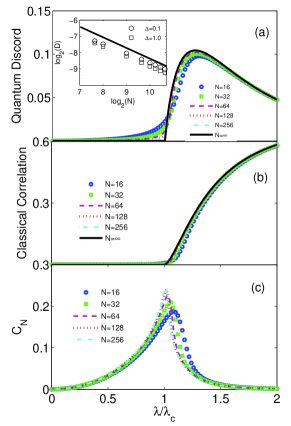
Figure 1: (Color online) (a) QD, (b) classical correlation, and (c) scaled concurrence as a function of the coupling constant in the Dicke model with different sizes for $\Delta=1.0$ and $\omega=1.0$. Inset in (a) is the finite-size scaling of the QD at the critical point $\lambda_{c}$, and the solid line scales as $N^{-2/3}$.

It is well known that the second-order QPT occurs in the thermodynamic limit. The quantum correlation is deeply related to QPT. The reminiscences of the QPT for a finite (large) system size should be very interesting. Therefore, we study the size dependence of the QD and classical correlation in the Dicke model. In Figs. 1(a) and 1(b), we display the quantum correlation and classical correlation as a function of the atom-cavity coupling constant for several system sizes. The results in the thermodynamic limit are also listed.

It is shown that both the quantum correlation and classical correlation are quite small in the normal phase ($\lambda<\lambda_{c}$). They tend to zero with the increase of the atomic number, agreeing well with the results in the thermodynamic limit, which is exactly zero. In the thermodynamic limit, there is no excitation of the system in the normal phase, so a correlation between two arbitrary atoms, which can only be mediated by the photons, should be absent. While in the superradiant phase ($\lambda>\lambda_{c}$), the QD shows nonmonotonous behavior as the coupling strength increases in Fig. 1(a). The maximum of the QD is away from the critical point, even in the thermodynamic limit, locating at $1.28\lambda_{c}$. This suggests that the nonclassical atom-atom correlation becomes strongest at the mediate coupling regime above the critical point. It is different from the one-dimensional XXZ model raoul1 , where the maximum of the QD is right at the critical point.

It is very interesting to observe a power-law scaling $\mathcal{D}|_{\lambda=\lambda_{c}}{\propto}N^{-{\mu}}$ for different detunings, as shown in the inset of Fig. 1(a). The asymptotic slop in the log-log scale in the large-size atomic systems for different detunings suggests the same exponent $\mu=2/3$. To the best of our knowledge, such a finite-size scaling for the QD itself has never been reported in other systems at critical regime. In the recent study on one dimensional XY model with symmetry-breaking longitudinal field in Ref. tomasello1 , an exponential scaling is observed near the factorization points, which provides a nontrivial scaling feature of the QD even in the noncritical regimes. This is significantly different from the results in the Dicke model, which holds at the critical point. Nevertheless, the ground state of this XY system at the factorization points is separable, resulting in the disappearance of the QD. This is similar to what happens in the Dicke model at the normal phase, where the atoms part of the ground state is dominated by the separable form ${\Pi^{N}_{k=1}}|{\downarrow}{\rangle}_{k}$, with $\sigma^{z}_{k}|{\downarrow}{\rangle}_{k}=-|{\downarrow}{\rangle}_{k}$.

As the coupling strength increases further, the QD becomes smaller. In the strong coupling limit, the QD finally decreases to zero, which means the nonlocal quantum correlation of the system disappears. In this limit ($\lambda{\gg}\lambda_{c}$), the ground state can be described by $|\psi^{\pm}_{G}{\rangle}=\frac{1}{\sqrt{2}}[(\Pi^{N}_{k=1}|{e_{x}}{\rangle}_{k})|0{\rangle}_{A_{-N/2}}{\pm}(\Pi^{N}_{k=1}|{g_{x}}{\rangle}_{k})|0{\rangle}_{A_{N/2}}]$ under $C_{2}$ symmetry Hirsch , where ${\sigma^{x}_{k}}|e_{x}{\rangle}_{k}=|e_{x}{\rangle}_{k}$ and ${\sigma^{x}_{k}}|g_{x}{\rangle}_{k}=-|g_{x}{\rangle}_{k}$. $|0{\rangle}_{A_{-N/2}}$ and $|0{\rangle}_{A_{N/2}}$ are the vacuum for the coherent state modes $A_{-N/2}|0{\rangle}_{A_{-N/2}}=0$ and $A_{N/2}|0{\rangle}_{A_{N/2}}=0$, respectively. Hence, the reduced bipartite density matrix of the arbitrary two atoms corresponds to complete einselection ollivier1 , where the QD appears zero. On the other hand, it can also be seen in Eq. (III) that $\beta^{2}=1/2$ as $\lambda{\rightarrow}\infty$, so $\mathcal{D}{\rightarrow}0$.

The classical correlation in the superradiant phase increases monotonously with the coupling strength, similar to those in the different spin chains raoul1 ; liu1 . In the thermodynamical limit, $\beta^{2}{\rightarrow}1/2$ in the deep coupling regime, so that $H(\mathcal{A})=H(\mathcal{B})=\ln 2$, and $H(\mathcal{A},\mathcal{B})=\ln 2$. For the conditional von Neumann entropy, $H(\mathcal{A}|\Pi^{\mathcal{B}})=0$. Hence, the classical correlation saturates at $\log 2$ in the strong coupling limit.

It is well known that the concurrence and the QD are both good measures to investigate the nonclassical correlations. Hence, comparisons between these two quantities are highly desirable. The scaled concurrence has been calculated previously by $C_{N}=1-4{\langle}J^{2}_{y}{\rangle}/N$ lambert1 . The scaled concurrence in the very large system size has been calculated later by two present authors and collaborators chen1 . We also collect the scaled concurrence as a function of coupling constant for different size in Fig. 1 (c) for convenience.

Interestingly, we find that QD and scaled concurrence show essentially different behaviors in the whole coupling regime. First, it is shown that the QD decreases with the atomic number in the normal phase and vanishes exactly in the thermodynamic limit. While the scaled concurrence increases with the atomic number in the normal phase, it is always finite in the thermodynamic limit. Since the scaled concurrence is defined by $C_{N}=(N-1)C_{n}$, where $C_{n}$ is the normal concurrence, it is given by a two-point entanglement measure times the system size (the atomic number). On the contrary, the QD is a measure of two-point nonclassical correlations and it is not multiplied by the atomic number. This clearly explains their different behaviors with respect to the increase of the system size. The normal concurrence $C_{n}$ is vanishing in the thermodynamic limit, implying that entanglement between two arbitrary atoms should be absent in this limit. This feature is consistent with the disappearance of the QD. Second, the scaled concurrence reaches its maximum at the critical point where the QD is still very small. Third, in the superradiant phase, the QD shows a broad maximum and decays slowly. The scaled concurrence decreases monotonically and rapidly with the coupling constant in the strong coupling regime. For example, for ${\lambda}/{\lambda_{c}}=2.0$, the scaled concurrence becomes negligible, and the value of the QD still remains about half of the maximum, demonstrating the persistence of the QD in regimes where entanglement is absent, a feature already observed in the extended Hubbard model allegra1 . Therefore we conclude that the scaled concurrence is not sufficient to quantify the nonclassical correlation. In this sense, one can say that QD is a pretty good measure of the quantum correlation independent of entanglement.

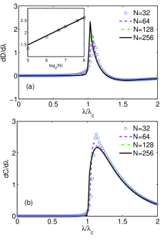
Figure 2: (Color online) First derivative of the QD (a) and the classical correlation (b) as a function of the coupling constant in the Dicke model with different system sizes for $\Delta=1.0$ and $\omega=1.0$. Inset in (a) shows the finite-size scaling of the maximum of the $d\mathcal{D}/d\lambda$.

To quantify the QPT of the Dicke model, the first derivative of the QD and the classical correlation as a function of the coupling constant are presented in Fig. 2. The cusplike peak of $\frac{d\mathcal{D}}{d\lambda}$ curves emerges with an increase of the atomic number, indicating a nonanalytical behavior. This feature confirms a general paradigm developed by Wu et al. wu1 . The peak position tends to the critical point with increasing $N$. It would provide a good tool to detect the critical point by a finite-size study. In the critical spin chains, the first derivative of the QD also shows its peak right at the critical point, which is also nonanalytical and discontinuous sarandy1 ; maziero1 ; tomasello1 ; liu1 ; li1 .

Interestingly, the logarithmic scaling of the maximum of the $d\mathcal{D}/d\lambda$ is also observed in the large size regime, which can be fitted well by $(\frac{d\mathcal{D}}{d\lambda})_{\textrm{max}}=0.377\ln_{2}(N)-0.401$, demonstrated in the inset of Fig. 2(a). This logarithmic scaling has been also reported in Refs. li1 ; sarandy1 for XY spin chains and transverse field Ising chains, implying the universal features of the derivatives of the QD to exhibit the novel behaviors of the critical systems. The first derivative of the classical correlation $\frac{d\mathcal{C}}{d\lambda}$ displays a different behavior. It becomes more rounded around the maximum with the increase of the size.

IV Quantum Correlation of the LMG Model

We turn to the other quantum collective spin model, the LMG model. Its Hamiltonian reads LMG ; Dusuel ; Leyvraz

$$H_{\text{LMG}}=-\frac{1}{2N}\sum_{i<j}({\sigma}^{x}_{i}{\sigma}^{x}_{j}+{\gamma}{\sigma}^{y}_{i}{\sigma}^{y}_{j})-\frac{\lambda}{2}\sum_{i}{\sigma}^{z}_{i}.$$ (21)

where $\sigma_{i}(i=x,y,z)$ are Pauli spin-$1/2$ operators, $\lambda$ is the magnetic field, and $\gamma$ is the anisotropic parameter. In the framework of the collective spin operators $J_{k}=\sum_{i}{\sigma^{k}_{i}}/2$ with $k=x,y,z$, the model can be rewritten as

$$H_{\text{LMG}} = -{\lambda}J_{z}-\frac{1}{N}[J^{2}_{x}+{\gamma}J^{2}_{y}-N(1+\gamma)/4].$$ (22)

We focus on the case of $\gamma=0$ and $\lambda>0$ where the second-order QPT can occur.

We also first study the quantum and classical correlation in the thermodynamic limit. Based on the Holstein-Primakoff transformation $J_{z}=b^{{\dagger}}b-N/2,J_{+}=b^{{\dagger}}\sqrt{N-b^{{\dagger}}b},J_{-}=\sqrt{N-b^{{\dagger}}b}b$, we displace the boson operator to the form of $c^{{\dagger}}=b^{{\dagger}}+\alpha$. By large $N$ expansion of $H_{\text{LMG}}$, the ground-state energy per spin is shown as

$$E_{G}/N=-[(1-\alpha^{2})\alpha^{2}+\lambda(\alpha^{2}-1/2)].$$ (23)

By minimizing $E_{G}$, we find

$$\alpha^{2}=\min\{1,\frac{1+\lambda}{2}\}.$$ (24)

Consequently, we have ${\langle}J_{z}{\rangle}/N=(\alpha^{2}-1/2),{\langle}J^{2}_{z}{\rangle}/N^{2}=(\alpha^{2}-1/2)^{2}$, and ${\langle}J^{2}_{+}{\rangle}/N^{2}=\alpha^{2}(1-\alpha^{2})$. Then the elements of the pairwise density matrix in Eq. (9) up to $O(1)$ are derived by

$$v_{+} = (\frac{1+\lambda}{2})^{2},~{}v_{-}=(\frac{1-\lambda}{2})^{2},$$ (25)

$$w = y=(\frac{1+\lambda}{2})(\frac{1-\lambda}{2}),~{}u=(\frac{1+\lambda}{2})(\frac{1-\lambda}{2}).$$

By a suitable reparametrization we cast the matrix elements in the same form as those of the Dicke model in Eq. (III)

$$\beta^{2} = \frac{1-\lambda}{2},~{}1-\beta^{2}=\frac{1+\lambda}{2}.$$ (26)

Therefore the elements can be expressed as

$$~{}v_{+} = (1-\beta^{2})^{2},~{}v_{-}=\beta^{4},$$ (27)

$$w = y=\beta^{2}(1-\beta^{2}),~{}u=\beta^{2}(1-\beta^{2}).$$

The influence of the anisotropic parameter $\gamma$ on the quantum correlation is numerically checked, and we find that the QD is almost not altered with $\gamma$. Hence we mainly focus on $\gamma=0$ in the following.

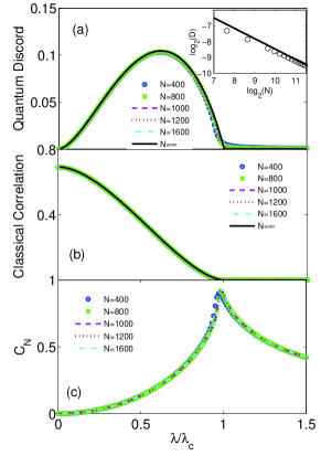
Figure 3: (Color online) (a) QD, (b) classical correlation, and (c) scaled concurrence as a function of the field in the LMG model with different system sizes for $\gamma=0$. Inset in (a) is the finite-size scaling of the QD at the critical point $\lambda_{c}$, and the solid line scales as $N^{-2/3}$.

The finite-size LMG model can be studied by the exact diagonalization on the basis of the collective spin operators Dusuel . For the ground state, convergent results can be obtained for very a large system size. The size dependence of the QD and the classical correlation are given in Fig. 3. The QD shows the nonmonotonous behavior in the symmetry-broken phase ($\lambda<\lambda_{c}$). Starting at $0$, the QD then shows the single broad maximum at $\lambda=0.62\lambda_{c}$, far from the critical point. The QD is very small in the symmetry phase ($\lambda>\lambda_{c}$). The classical correlation decreases monotonously in the symmetry-broken phase, approaching to zero at the critical point. If the magnetic field $\lambda=0$, the classical correlation is easily obtained as $\ln 2$. In the symmetry phase, the classical correlation is rather small for a finite-size system and becomes zero in the thermodynamic limit.

Similar to the Dicke model, the QD of the LMG model also exhibits the power-law scaling behavior as $\mathcal{D}_{\lambda=\lambda_{c}}{\propto}N^{-\mu}$ at the critical point, as shown in the inset of Fig. 3(a). The scaling exponent $\mu$ in the large $N$ regime is very close to $2/3$, the same as that obtained above in the Dicke model, providing a new piece of evidence of the same universality class of these two models.

The QD in the LMG model in the thermodynamic limit has been preliminarily studied in Ref. sarandy1 . By mapping the LMG model to the two-band fermion model exactly, the quantum correlation and the classical correlation of the fermions were studied alternatively, based on the corresponding density matrix. It was found that both the QD and the classical correlation decrease monotonously in the symmetry-broken phase with the magnetic field, and keep zero in the symmetry-broken phase. In the present paper, the pairwise density matrix in the LMG model is evaluated directly for qubits (i.e., spins) and it is related, but not identical to that of Ref. sarandy1 . The different definitions may account for the different values of QD obtained in the two papers. Our results for the classical correlation are consistent qualitatively with those in Ref. sarandy1 .

The comparisons of the QD and the scaled concurrence in the LMG model are also made. The scaled concurrence for large system size has been calculated by Dusuel et al. Dusuel1 , which was shown in their Fig. 9. For completeness, we recalculate the concurrence, also including much larger system sizes, and list them in Fig. 3(c). At the critical point, the concurrence shows the maximum, while the QD becomes $0$. In the symmetry phase ($\lambda>\lambda_{c}$), the QD is very small, implying no quantum correlation. The concurrence remains finite and decreases gradually and monotonously with the field $\lambda$.

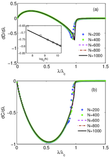
Figure 4: (Color online) First-order derivative of the QD (a) and the classical correlation (b) as a function of the field in the LMG model with different system sizes for $\gamma=0$. Inset in (a) exhibits the finite-size scaling of the minimum of the $d\mathcal{D}/d\lambda$.

In order to study the critical behaviors of the LMG model, we display the first derivative of the QD and classical correlation in Fig. 4. $\frac{d\mathcal{D}}{d\lambda}$ has a pronounced minimum around the critical point. Note that the minimum position approaches the critical point, providing a convincing method to locate the critical point. This behavior strongly mirrors the sudden transition from the symmetry-broken phase to the symmetric phase. The finite-size scaling of the minimum of the $d{\mathcal{D}/d\lambda}$ is also performed in the inset of Fig. 3. The logarithmic divergence fitted by $(\frac{d\mathcal{D}}{d\lambda})_{\textrm{min}}=-0.044\ln_{2}(N)-0.346$ is also well exhibited in the large size regime, similar to that in the Dicke model. It should be pointed out that the coefficients of $\ln_{2}(N)$ in the two models are different. The first derivative of the classical correlation shows the broad valley around $0.55\lambda_{c}$, and becomes $0$ as the field parameter $\lambda\geq\lambda_{c}$. Combined with the similar scaling behavior reported in spin chains li1 ; sarandy1 , such a logarithmic divergence of the first derivative of the QD may be universal in critical systems; further extensive confirmations in other systems are, however, needed.

V Summary

The QD and the classical correlation are investigated to characterize QPTs in the Dicke model and the LMG model. These correlations in the thermodynamic limit have been derived analytically and in the finite-size system obtained numerically up to very a large system size. Perfect power-law scaling behavior at the critical point is observed in both models. Such a scaling behavior has not been reported in other critical systems, except the exponential scaling at noncritical regimes in the XY chain with symmetry-breaking field tomasello1 . The same scaling exponents provide new evidence of the same universality of two models. The position of the pronounced maximum or minimum of the first derivative of the QD approaches to the critical point with the increase of the system size, unlike some other critical systems. We have convincing evidence of a logarithmic diverging behavior for the first derivative of the QD in the two models. It is suggested that this logarithmic diverging behavior at the critical point might be universal in the second QPTs. The coefficient of the logarithmic term is, however, model dependent.

We also find that the QD and the scaled concurrence show essentially different behaviors in both models. In the symmetry phase, the QD vanishes in the thermodynamic limit, while the scaled concurrence remains finite. In the symmetry-breaking phase, the QD shows the broad maximum and becomes zero in the strong atom-cavity (atom-atom) coupling limit, whereas the scaled concurrence decreases monotonically. This explicitly shows the robustness of the QD in the symmetry-breaking phase, compared to the scaled concurrence. Recently, we note that the multipartite measure (global quantum discord) emerges as a powerful tool for quantum correlation rulli1 . Hence, it may be interesting to apply the global quantum discord to further exploit the novel behaviors in collective spin systems in future research.

VI Acknowledgement

This work was supported by National Natural Science Foundation of China

Appendix A Derivation of the quantum correlation

Considering the pairwise atom reduced density matrix in Eq. (9), the reduced density matrix ${\rho}_{\mathcal{A}}$ is obtained by

$${\rho}_{\mathcal{A}} = \text{Tr}_{\mathcal{B}}\{{\rho}_{\mathcal{A},\mathcal{B}}\}$$

$$= (v_{+}+w)|\downarrow{\rangle}_{\mathcal{A}}{\langle}\downarrow|+(v_{-}+w)|\uparrow{\rangle}_{\mathcal{A}}{\langle}\uparrow|.$$

The Von Neumann entropy of the reduced system $\mathcal{A}$ is shown as

$$~{}H(\mathcal{A}) = -(v_{+}+w)\ln(v_{+}+w)-(v_{-}+w)\ln(v_{-}+w).$$

The joint von Neumann entropy can be derived from the joint pairwise matrix in (Eq. (9)), by which we have

$$(\lambda+y-w)[(w-\lambda)+y][(\lambda-v_{+})(\lambda-v_{-})-|u|^{2}]=0.$$

The eigenvalues ${\lambda_{i}}(i=1,2,3,4)$ can be obtained analytically. Then the joint entropy is demonstrated as

$$H(\mathcal{A},\mathcal{B}) = -(w+y)\ln(w+y)-(w-y)\ln(w-y)$$

$$-\sum_{\lambda=\lambda_{\pm}}{\lambda}\ln{\lambda},$$

where $\lambda_{\pm}=\frac{1}{2}\{(v_{+}+v_{-}){\pm}[(v_{+}-v_{-})^{2}+4|u|^{2}]^{1/2}\}$.

The conditional density ${\rho}_{\mathcal{A}|{\Pi}^{\mathcal{B}}_{k}}$ is measured by the projections tuned by $\theta$ and $\phi$

$$|\Psi_{1}{\rangle}_{\mathcal{B}} = \cos(\theta)|\downarrow{\rangle}_{\mathcal{B}}+e^{i\phi}\sin(\theta)|\uparrow{\rangle}_{\mathcal{B}}~{}$$

$$|\Psi_{2}{\rangle}_{\mathcal{B}} = e^{-i\phi}\sin(\theta)|\downarrow{\rangle}_{\mathcal{B}}-\cos(\theta)|\uparrow{\rangle}_{\mathcal{B}}.$$

Under such projections, the conditional density matrix is shown as

$$~{}{\rho}_{\mathcal{A}|{\Pi}^{\mathcal{B}}_{\Psi_{\alpha}}} = |\Psi_{\alpha}{\rangle}_{\mathcal{B}}{\langle}\Psi_{\alpha}|\{|\downarrow{\rangle}_{\mathcal{A}}{\langle}\downarrow|X_{\alpha,+}+|\uparrow{\rangle}_{\mathcal{A}}{\langle}\uparrow|X_{\alpha,-}$$

$$+|\downarrow{\rangle}_{\mathcal{A}}{\langle}\uparrow|Y_{\alpha}+|\uparrow{\rangle}_{\mathcal{A}}{\langle}\downarrow|Y^{*}_{\alpha}\}/p_{\alpha}.$$

For ${\alpha}=1$,

$$X_{1,+} = v_{+}{\cos}^{2}(\theta)+w{\sin}^{2}(\theta),$$ (28)

$$X_{1,-} = w{\cos}^{2}(\theta)+v_{-}{\sin}^{2}(\theta),$$

$$Y_{1} = {\sin}(\theta){\cos}(\theta)[e^{i\phi}u^{*}+e^{-i\phi}y],$$

$$p_{1} = w+v_{+}{\cos}^{2}(\theta)+v_{-}{\sin}^{2}(\theta).$$

For ${\alpha}=2$,

$$X_{2,+} = v_{+}{\sin}^{2}(\theta)+w{\cos}^{2}(\theta),$$ (29)

$$X_{2,-} = w{\sin}^{2}(\theta)+v_{-}{\cos}^{2}(\theta),$$

$$Y_{2} = -{\sin}(\theta){\cos}(\theta)[e^{i\phi}u^{*}+e^{-i\phi}y],$$

$$p_{2} = w+v_{+}{\sin}^{2}(\theta)+v_{-}{\cos}^{2}(\theta).$$

Then the eigenvalues of the conditional density matrix read

$$~{}~{}{\lambda}^{\alpha}_{\pm}(\theta,\phi) = \frac{1}{2p_{\alpha}}\{(X_{\alpha,+}+X_{\alpha,-}){\pm}[(X_{\alpha,+}-X_{\alpha,-})^{2}$$ (30)

$$+4|Y_{\alpha}|^{2}]^{1/2}\}.$$

The conditional von Neumann entropy is shown as

$$H(\mathcal{A}|\{{\Pi}^{\mathcal{B}}_{k}\})(\theta,\phi) = -\sum_{\alpha=1,2}p_{\alpha}[{\lambda}^{\alpha}_{+}(\theta,\phi){\ln}{\lambda}^{\alpha}_{+}(\theta,\phi)$$

$$+{\lambda}^{\alpha}_{-}(\theta,\phi){\ln}{\lambda}^{\alpha}_{-}(\theta,\phi)].$$

Hence

$$\delta(\theta,\phi)=H(\mathcal{A})-H(\mathcal{A},\mathcal{B})+H(\mathcal{A}|{\Pi}^{\mathcal{B}}).$$

Finally, the QD can be obtained by optimizing the $\theta$ and $\phi$ both in the regime $[0,{\pi}/2]$ to minimize $\delta(\theta,\phi)$, shown as

$$\mathcal{D}=\min_{\{\theta,\phi\}}\{\delta(\theta,\phi)\}.$$

Consequently, the corresponding classical correlation can also be obtained by

$$\mathcal{C}=\max_{\{\theta,\phi\}}\{H(\mathcal{A})+H(\mathcal{B})-H(\mathcal{A},\mathcal{B})-\delta(\theta,\phi)\}.$$

Appendix B Minimization of the conditional entropy in thermodynamic limit

In the thermodynamic limit, all non-zero elements of the pairwise density matrix in Eq. (9) have been derived in Eq. (III). So we can arrive at Eqs. (28) and (29)

$$(X_{k,+}+X_{k,-}) = {\eta}_{k}(\theta),$$

$$(X_{k,+}-X_{k,-}) = (2{\beta}^{2}-1){\eta}_{k}(\theta),$$

$$|Y_{k}|^{2} = |Y|^{2}={\beta}^{4}(1-{\beta}^{2})^{2}{\sin}^{2}{2\theta}{\cos}^{2}{\phi},$$

$$p_{k} = {\eta}_{k}(\theta),$$

where $\eta_{k}(\theta)=\frac{1}{2}[1+(-1)^{k-1}(2{\beta}^{2}-1){\cos}{2\theta}]$, with $k=1,2$. Therefore the eigenvalues of the conditional density matrix in Eq. (30) are obtained as

$${\lambda}^{k}_{\pm}(\theta,\phi) = \frac{{\eta}_{k}(\theta){\pm}[(2{\beta}^{2}-1)^{2}{\eta}^{2}_{k}(\theta)+4|Y|^{2}]^{1/2}}{2p_{k}}$$

$$= \frac{{\eta}_{k}(\theta)}{2p_{k}}\{1{\pm}[(2{\beta}^{2}-1)^{2}+\frac{4|Y|^{2}}{{\eta}^{2}_{k}(\theta)}]^{1/2}\},$$

which can be reduced to $\lambda^{k}_{\pm}(\theta,\phi)=\frac{{\eta}_{k}(\theta)}{2p_{k}}[1{\pm}x_{k}(\theta,\phi)]$ by defining $x_{k}(\theta,\phi)=[(2{\beta}^{2}-1)^{2}+\frac{4|Y|^{2}}{{\eta}^{2}_{k}(\theta)}]^{1/2}$ $(0{<}x_{k}{<}1)$. The conditional von Neumann entropy is described as

$$H(\mathcal{A}|\{\Pi^{\mathcal{B}}\})(\theta,\phi)$$

$$= \sum_{k=1,2}\{{\eta_{k}}(\theta)\ln{\eta_{k}}(\theta)$$

$$-[\frac{{\eta}_{k}(\theta)}{2}(1{+}x_{k}(\theta,\phi))]{\ln}[\frac{{\eta}_{k}(\theta)}{2}(1{+}x_{k}(\theta,\phi))]$$

$$-[\frac{{\eta}_{k}(\theta)}{2}(1{-}x_{k}(\theta,\phi))]{\ln}[\frac{{\eta}_{k}(\theta)}{2}(1{-}x_{k}(\theta,\phi))]\}$$

$$= {\ln}{2}-\sum_{k=1,2}\frac{\eta_{k}(\theta)}{2}[(1{+}x_{k}(\theta,\phi)){\ln}(1{+}x_{k}(\theta,\phi))$$

$$+(1{-}x_{k}(\theta,\phi)){\ln}(1{-}x_{k}(\theta,\phi))],$$

Since $F(x)=-[(1+x)\ln(1+x)+(1-x)\ln(1-x)]$ is the monotonically decreasing function, $\phi$ is selected to $0$ to maximize $x_{k}(\theta,\phi)$. Furthermore, we find $\theta=\pi/4$ to minimize the conditional von Neumann entropy as luo1

$$H(\mathcal{A}|\Pi^{\mathcal{B}}) = \ln(2)-\frac{1}{2}[(1+M)\ln(1+M)~{}$$

$$+(1-M)\ln(1-M)],$$

where $M=x(\pi/4,0)=[(2{\beta}^{2}-1)^{2}+16{\beta}^{4}(1-{\beta}^{2})^{2}]^{1/2}$.

References

- (1) P. L. Taylor and O. Heinonen, A Quantum Approach to Condensed Matter Physics (Cambridge University Press, Cambridge, UK, 2002).
- (2) M. A. Nielsen and I. L. Chuan, Quantum Computational and Quantum information (Cambridge University Press, Cambridge, UK 2000).
- (3) S. Sachdev, Quantum Phase Transitions (Cambridge University Press, Cambridge, UK, 2001).
- (4) K. Modi, A. Brodutch, H. Cable, T. Paterek, and V. Vedral, e-print arXiv:1112.6238 (to be published).
- (5) L. Amico, R. Fazio, A. Osterloh, and V. Vedral, Rev. Mod. Phys. 80, 517 (2008).
- (6) A. Osterloh, L. Amico, G. Falci, and R. Fazio, Nature (London) 416, 608 (2002).
- (7) S. J. Gu, H. Q. Lin, and Y. Q. Li, Phys. Rev. A 68, 042330 (2003).
- (8) L. A. Wu, M. S. Sarandy, and D. A. Lidar, Phys. Rev. Lett. 93, 250404 (2004).
- (9) S. J. Gu, S. S. Deng, Y. Q. Li, and H. Q. Lin, Phys. Rev. Lett. 93, 086402 (2004).
- (10) Ö. Legeza and J. Sólyom, Phys. Rev. Lett. 96, 116401 (2006).
- (11) J. Vidal, Phys. Rev. A 73, 062318 (2006).
- (12) H. Ollivier and W. H. Zurek, Phys. Rev. Lett. 88, 017901 (2001).
- (13) J. Oppenheim, M. Horodecki, P. Horodecki, and R. Horodecki, Phys. Rev. Lett. 89, 180402 (2002).
- (14) A. Datta, A. Shaji, and C. M. Caves, Phys. Rev. Lett. 100, 050502 (2008).
- (15) B. P. Lanyon, M. Barbieri, M. P. Almeida, and A. G. White, Phys. Rev. Lett. 101, 200501 (2008).
- (16) T. Werlang and G. Rigolin, Phys. Rev. A 81, 044101 (2010).
- (17) T. Werlang, C. Trippe, G. A. P. Ribeiro, and G. Rigolin, Phys. Rev. Lett. 105, 095702 (2010); T. Werlang, G. A. P. Ribeiro, and G. Rigolin, Phys. Rev. A 83, 062334 (2011).
- (18) R. Dillenschneider, Phys. Rev. B 78, 224413 (2008).
- (19) M. S. Sarandy, Phys. Rev. A 80, 022108 (2009).
- (20) L. Amico, D. Rossini, A. Hamma, and V. E. Korepin, e-print arXiv:1112.3280 (to be published).
- (21) J. Maziero, H. C. Guzman, L. C. Céleri, M. S. Sarandy, and R. M. Serra, Phys. Rev. A 82, 012106 (2010).
- (22) B. Tomasello, D. Rossini, A. Hamma, L. Amico, Europhys. Lett. 96, 27002 (2011); e-print arXiv:1112.0361 (to be published).
- (23) B. Q. Liu, B. Shao, J. G. Li, J. Zou, and L. A. Wu, Phys. Rev. A 83, 052112 (2011).
- (24) Y. C. Li and H. Q. Lin, Phys. Rev. A 83, 052323 (2011).
- (25) M. Allegra, P. Giorda, and A. Montorsi, Phys. Rev. B 84, 245133 (2011).
- (26) Y. X. Chen and S. W. Li, Phys. Rev. A 81, 032120 (2010).
- (27) R. H. Dicke, Phys. Rev. 93, 99 (1954).
- (28) H. J. Lipkin, N. Meshkov, and A. J. Glick, Nucl. Phys. 62, 188 (1965).
- (29) J. I. Cirac, M. Lewenstein, K. Mølmer, and P. Zoller, Phys. Rev. A 57, 1208 (1998).
- (30) S. Dusuel and J. Vidal, Phys. Rev. Lett. 93, 237204 (2004).
- (31) F. Leyvraz and W. D. Heiss, Phys. Rev. Lett. 95, 050402 (2005).
- (32) G. Vidal, J. I. Latorre, E. Rico, and A. Kitaev, Phys. Rev. Lett. 90, 227902 (2003).
- (33) K. Baumann, C. Guerlin, F. Brennecke, and T. Esslinger, Nature (London) 464, 1301 (2010); K. Baumann, R. Mottl, F. Brennecke, and T. Esslinger, Phys. Rev. Lett. 107, 140402 (2011).
- (34) P. Strack and S. Sachdev, Phys. Rev. Lett. 107, 277202 (2011).
- (35) J. Reslen, J. Quiroga, and N. F. Johnson, Europhys. Lett. 69, 8 (2005); J. Vidal and S. Dusuel, Europhys. Lett. 74, 817 (2006); T. Barthel, S. Dusuel, and J. Vidal, Phys. Rev. Lett. 97, 220402 (2006).
- (36) J. Wilms, J. Vidal, F. Verstraete and S. Dusuel, J. Stat. Mech. P01023 (2012).
- (37) W. H. Zurek, Phys. Rev. A 67, 012320 (2003).
- (38) X. Wang and K. Mølmer, Eur. Phys. J. D 18, 385 (2002).
- (39) S. L . Luo, Phys. Rev. A 77, 042303 (2008); M. Ali, A. R. P. Rau, and G. Alber, Phys. Rev. A 81, 042105 (2010); F. F. Fanchini, T. Werlang, C. A. Brasil, L. G. E. Arruda, and A. O. Caldeira, Phys. Rev. A 81, 052107 (2010).
- (40) C. Emary and T. Brandes, Phys. Rev. E 67, 066203 (2003); Phys. Rev. Lett. 90, 044101 (2003).
- (41) Q. H. Chen, Y. Y. Zhang, T. Liu, and K. L. Wang, Phys. Rev. A 78, 051801(R) (2008).
- (42) M. A. Bastarrachea-Magnani and J. G. Hirsch, e-print arXiv:1108.0703 (to be published).
- (43) N. Lambert, C. Emary, and T. Brandes, Phys. Rev. Lett. 92, 073602 (2004).
- (44) S. Dusuel and J. Vidal, Phys. Rev. B 71, 224420 (2005).
- (45) C. C. Rulli and M. S. Sarandy, Phys. Rev. A 84, 042109 (2011); A. Saguia, C. C. Rulli, T. R. de Oliveira, and M. S. Sarandy, Phys. Rev. A 84, 042123 (2011).