Accelerating the convergence of path integral dynamics with a generalized Langevin equation

Abstract

The quantum nature of nuclei plays an important role in the accurate modelling of light atoms such as hydrogen, but it is often neglected in simulations due to the high computational overhead involved. It has recently been shown that zero-point energy effects can be included comparatively cheaply in simulations of harmonic and quasi-harmonic systems by augmenting classical molecular dynamics with a generalized Langevin equation (GLE). Here we describe how a similar approach can be used to accelerate the convergence of path integral (PI) molecular dynamics to the exact quantum mechanical result in more strongly anharmonic systems exhibiting both zero point energy and tunnelling effects. The resulting PI-GLE method is illustrated with applications to a double-well tunnelling problem and to liquid water.

I Introduction

Atomistic computer simulations have become an important complement to experimental measurements in studies of a wide variety of physical, chemical and biological systems. However, in order to reduce computational effort that is required for larger systems, a number of approximations are typically made in these simulations. One that is commonly employed is to assume that the atomic nuclei behave as classical particles, even when the interactions between them are obtained from an ab initio calculation. This is a reasonable assumption for heavy atoms at high temperatures. But for lighter atoms – and hydrogen in particular – significant deviations are to be expected from classical behavior even at room temperature.

When empirical interaction potentials are used to compute the forces acting on the nuclei, nuclear quantum effects are often implicitly accounted for, because force fields are typically parameterised so as to agree with experimental data when used in classical molecular dynamics simulations. When ab initio methods are used to describe the interactions between the nuclei, there is no such parameterisation for nuclear quantum effects, and the error that results from assuming purely classical behavior of the nuclear motion is often comparable to that stemming from an approximate treatment of electron correlation.Morrone and Car (2008)

The conventional approach to including nuclear quantum effects exploits the isomorphism between the quantum mechanical partition function of the physical system and the classical partition function of an extended problem consisting of a necklace (or ring polymer) of replicas of the system in which corresponding atoms are connected by harmonic springs.Chandler and Wolynes (1981) As the number of replicas (or beads of the necklace) is increased, this imaginary time path integralFeynman and Hibbs (1965) (PI) method samples an ensemble that converges systematically to that of the quantum problem with distinguishable particles, at the expense of a computational effort that increases in proportion to the number of beads.

Methods have been devised to reduce this effort by splitting the calculation of forces into an inexpensive, short-ranged contribution that is computed on every bead, and a long-range contribution that is evaluated on a contracted ring polymer with fewer beads.Markland and Manolopoulos (2008a, b); Fanourgakis, Markland, and Manolopoulos (2009) These methods are straightforward to implement in simulations with empirical force fields. However they cannot presently be used in ab initio simulations, where the splitting of the forces into an inexpensive short-range contribution plus a more expensive long-range contribution is significantly more difficult to arrange. Approximate quantum methods such as the Feynman-HibbsFeynman and Hibbs (1965); Voth (1991) approach are also difficult to use in ab initio simulations, because they require the computation of the Hessian.

A more general approach to reducing the effort of path integral simulations is therefore called for, and there are certain indications in the literature that this might now be possible. In particular, it has recently been shown that colored noise, generalized Langevin equation (GLE) thermostats can be used not only to enhance the sampling of classical and path integral molecular dynamics,Ceriotti, Bussi, and Parrinello (2010); Ceriotti et al. (2010a) but also to modify conventional molecular dynamics so as to include nuclear quantum effects in mildly anharmonic systems in which zero-point energy plays a significant role.Ceriotti, Bussi, and Parrinello (2009a) This approach involves negligible overhead with respect to purely classical dynamics, provides very naturally the proton momentum distribution (which is relevant for comparison with inelastic neutron scattering experiments), and can be applied with the same ease to empirical and ab initio force fields. However, it does not provide a satisfactory description of more subtle quantum effects such as tunnelling, and its accuracy cannot be systematically improved.

In this paper, we will show that it is possible to combine a GLE thermostat with path integral molecular dynamics (PIMD) in such a way as to exploit the best features of both techniques. In particular, by tuning the properties of the correlated noise in an appropriate GLE, we will show that the systematic convergence of PIMD to the exact quantum mechanical result can be greatly accelerated, leading to significant computational savings for a given level of accuracy. The resulting PI+GLE scheme provides an equally reliable description of zero point energy and tunnelling effects, it is equally applicable to simulations with empirical and ab initio force fields, and unlike the original single-bead “quantum thermostat” discussed above it can be systematically improved simply by increasing the number of path integral beads.

The outline of the paper is as follows. In Section II we briefly recall a few concepts from path integral and generalized Langevin equation methods, and describe our strategy to have them work in synergy. In Section III we present a systematic study of a one-dimensional quartic double well potential, discussing the effect of zero point energy and tunnelling on the convergence of our method. In Section IV we examine how the method performs for liquid water, and in Section V we draw our conclusions.

II Combining path integrals with the generalized Langevin equation

II.1 Path integral methods

Let us first recall the basic principles of imaginary time path integral methods, so as to introduce our notation. We will only discuss the one-dimensional case and refer the reader to the literatureFeynman and Hibbs (1965); Barker (1979); Chandler and Wolynes (1981); Par ; Parrinello and Rahman (1984); Ceperley (1995); Schulman (2005) for a more detailed discussion.

Consider the Hamiltonian for a particle in a one-dimensional potential,

$$\hat{H}=\frac{1}{2}\hat{p}^{2}+V(\hat{q}),$$ (1)

where $\hat{p}$ and $\hat{q}$ are the mass-scaled momentum and position operators and the potential $V(q)$ is assumed to be such that the quantum mechanical partition function

$$Z=\mathrm{tr}\bigl{[}e^{-\hat{H}/k_{B}T}\bigr{]}$$ (2)

is well defined. The path integral formalism avoids the solution of the Schrödinger equation for the Hamiltonian in Eq. (1) and allows one instead to sample configurations consistent with the quantum mechanical equilibrium distribution by exploiting an isomorphism with an extended classical problem.Chandler and Wolynes (1981) Indeed a standard Trotter-productSchulman (2005) approximation to the Boltzmann operator in Eq. (2) yields the following extended phase space expression for the partition function

$$Z\approx Z_{P}=\frac{1}{(2\pi\hbar)^{P}}\int\mathrm{d}^{P}\mathbf{p}\int\mathrm{d}^{P}\mathbf{q}\,e^{-H_{P}(\mathbf{p},\mathbf{q})/Pk_{B}T},$$ (3)

where $H_{P}(\mathbf{p},\mathbf{q})$ is the classical Hamiltonian of a fictitious ring polymer composed of $P$ replicas of the system connected by harmonic springs

$$H_{P}(\mathbf{p},\mathbf{q})=\sum_{j=0}^{P-1}\left[\frac{1}{2}p_{j}^{2}+V(q_{j})+\frac{1}{2}\omega_{P}^{2}(q_{j}-q_{j+1})^{2}\right],$$ (4)

with $\omega_{P}=Pk_{B}T/\hbar$ and $q_{P}\equiv q_{0}$. The error in this approximation is $O(P^{-2})$ and so vanishes to leave the exact quantum mechanical result in the limit as $P\to\infty$.Schulman (2005)

The momenta are often integrated out of Eq. (3) to leave a purely configurational integral which forms the basis of the path integral Monte Carlo (PIMC) technique.Barker (1979) One can however retain the momenta, and describe the dynamical evolution of the ring polymer by means of Hamilton’s equations. This is the PIMD approach,Par ; Parrinello and Rahman (1984) which provides a particularly efficient way to sample the configuration space in situations such as molecular liquid simulations in which an effective PIMC calculation would require complicated collective moves. A fully converged PIMD calculation produces the exact thermodynamic and structural properties of the quantum mechanical system. Although it is something of an aside to the present work, in which we shall be concerned exclusively with static equilibrium properties, it is also now well established that the centroid molecular dynamicsCao and Voth (1994); Jang and Voth (1999) and ring polymer molecular dynamicsCraig and Manolopoulos (2004); Braams and Manolopoulos (2006) generalizations of PIMD can be used to provide quite reasonable estimates of dynamical properties such as diffusion coefficients and chemical reaction rates.

The extension to three dimensions and to an arbitrary number of interacting distinguishable particles is straightforward. But rather than describe this extension here, let us consider instead the simple case of a one-dimensional harmonic potential, $V(q)=\omega^{2}q^{2}/2$. The result will be used in what follows. For this simple model, the integral in Eq. (3) can be evaluated by transforming to the $P$ normal modes $\{q_{k}\}_{0}^{P-1}$ of the ring polymer with frequencies

$$\omega_{k}=\sqrt{\omega^{2}+4\omega_{P}^{2}\sin^{2}(k\pi/P)}.$$ (5)

It is then easy to show that the equilibrium position distribution of each bead of the ring polymer will be a Gaussian centred on $q=0$, with a variance

$$\left<q^{2}\right>_{P}={1\over P}\sum_{k=0}^{P-1}\left<q_{k}^{2}\right>=k_{B}T\sum_{k=0}^{P-1}\frac{1}{\omega_{k}^{2}},$$ (6)

which converges to the correct quantum mechanical thermal expectation value

$$\left<q^{2}\right>={\hbar\over 2\omega}\coth{\hbar\omega\over 2k_{B}T}$$ (7)

in the limit as $P\to\infty$.

II.2 Generalized Langevin equations

It has recently been shown that an appropriate generalized Langevin equation (GLE) thermostat can be used to sample configurations for a harmonic oscillator that are consistent with the quantum mechanical variance in Eq. (7) using just a single replica of the system, thereby avoiding the overhead of a $P$-bead PI simulation.Ceriotti, Bussi, and Parrinello (2009a)

The basic idea behind GLE thermostats is to construct a linear, Markovian stochastic differential equation (SDE) in an extended momentum space which is coupled to the Hamiltonian dynamics in such a way that the equations of motion read

$$\begin{split}\dot{q}=&\ p\\ \!\left(\!\begin{array}[]{c}\dot{p}\\ \dot{\mathbf{s}}\end{array}\!\right)\!=&\left(\!\begin{array}[]{c}-V^{\prime}(q)\\ \mathbf{0}\end{array}\!\!\right)\!-\!\left(\!\begin{array}[]{cc}a_{pp}&\mathbf{a}_{p}^{T}\\ \bar{\mathbf{a}}_{p}&\mathbf{A}\end{array}\!\right)\!\left(\!\begin{array}[]{c}p\\ \mathbf{s}\end{array}\!\right)\!+\!\left(\!\begin{array}[]{cc}b_{pp}&\mathbf{b}_{p}^{T}\\ \bar{\mathbf{b}}_{p}&\mathbf{B}\end{array}\!\right)\!\left(\!\begin{array}[]{c}\hbox{\multirowsetup$\boldsymbol{\xi}$}\\ \\ \end{array}\!\right),\end{split}$$ (8)

where $\boldsymbol{\xi}$ is a vector of $n+1$ uncorrelated Gaussian random numbers with $\left<\xi_{i}\left(t\right)\xi_{j}\left(0\right)\right>=\delta_{ij}\delta\left(t\right)$. It can be shown that the resulting trajectories are statistically equivalent to those obtained from a non-Markovian Langevin equation involving only $p$ and $q$,Zwanzig (2001)

$$\begin{split}\dot{q}=&\ p\\ \dot{p}=&-V^{\prime}(q)-\int_{-\infty}^{t}K(t-s)p(s)\mathrm{d}s+\zeta(t),\end{split}$$ (9)

where the friction kernel $K(t)$ and the noise correlation function $H(t)=\left<\zeta(t)\zeta(0)\right>$ are related by analytical expressions to the matrices that appear in Eq. (8). These relationships, together with a more detailed discussion, can be found in Ref. Ceriotti, Bussi, and Parrinello (2010)

The only non-linear term in Eq. (8) is the force $V^{\prime}(q)$. If the potential is harmonic, the force depends linearly on $q$, and the whole set of equations describe an Ornstein-Uhlenbeck process,Gardiner (2003) which can be solved analytically to yield closed-form expressions for static and dynamic properties of the trajectory. Based on these expressions, one can iteratively refine the parameters $a_{p}$, ${\bf a}_{p}^{T}$, $\overline{\bf a}_{p}$, ${\bf A}$, $b_{p}$, ${\bf b}_{p}^{T}$, $\overline{\bf b}_{p}$ and ${\bf B}$ in Eq. (8) subject to certain positivity constraints until the desired response of the thermostat is obtained.Ceriotti, Bussi, and Parrinello (2010)

When considering the generalisation of this strategy to a multi-dimensional harmonic problem, one realises that, because of the linear nature of the SDE and of the consequent rotational invariance, the dynamics will conform to the analytical predictions obtained from the Ornstein-Uhlenbeck process even if the thermostats are applied to Cartesian coordinates, without the need to diagonalise the Hessian and transform to normal modes. Moreover, it has been demonstrated in previous work that the analytical properties of the thermostat obtained in the harmonic limit provide a meaningful prediction of its behavior for anharmonic problems with a similar range of frequencies.Ceriotti, Bussi, and Parrinello (2010)

By employing this strategy it is possible to obtain a number of useful effects, such as efficient sampling of the canonical distribution in constant-temperature MD. In this application, a fluctuation-dissipation theorem must hold, which relates the friction kernel and the memory of the noise in Eq. (9) through $H(t)=k_{B}TK(t)$. More generally, when this condition is not imposed, one obtains a non-equilibrium dynamics in which a frequency-dependent effective temperature is enforced. Either way, one can calculate the stationary covariance of the harmonic dynamics in the $(q,p,\mathbf{s})$ extended phase space, and the mean squared fluctuations of the positions and momenta, which we will label $c_{qq}(\omega)$ and $c_{pp}(\omega)$, respectively. It is then possible to design a GLE dynamics which behaves as a “quantum thermostat”;Ceriotti, Bussi, and Parrinello (2009a) i.e., which enforces probability distributions of positions and momenta that are consistent with those expected for a quantum harmonic oscillator,

$$c_{qq}(\omega)=\frac{1}{\omega^{2}}c_{pp}(\omega)=\frac{\hbar}{2\omega}\coth\frac{\hbar\omega}{2k_{B}T},$$ (10)

and does so over a wide range of frequencies.

When applying this idea to a multi-dimensional system one faces the problem of zero-point energy leakage.Habershon and Manolopoulos (2009) Anharmonic coupling causes a flow of heat from high-frequency to low-frequency vibrations, and a departure from the desired behavior in Eq. (10). This problem can be mitigated to some extent by exploiting the flexibility of the GLE in Eq. (8) to enhance the coupling strength of the thermostat and ensure that all vibrations are maintained at the correct effective temperature. This approach has been shown to give satisfactory results in a number of realistic, condensed-matter applications, ranging from the calculation of diamond-graphite coexistence curvesKhaliullin et al. (2010) to the proton momentum distribution in hydrogen-storage materials.Ceriotti et al. (2010b)

Being simple to implement and computationally inexpensive, this “quantum thermostat” is an important step towards a routine treatment of nuclear quantum effects in molecular dynamics. It lacks however two desirable features; namely, the possibility of treating more subtle quantum effects such as tunnelling, and the possibility of increasing the accuracy in a systematic way. Since both these requirements are met by PI methods, one suspects that it might be possible to develop a synergistic approach which combines path integrals with the GLE thermostat so as to obtain accurate results without the effort of a fully-converged PI simulation. The implementation of such a PI+GLE approach is the subject of the next section.

II.3 A synergistic combination

When a GLE thermostat is applied to a path integral molecular dynamics simulation, the internal frequencies of the ring polymer necklace will be present along with the physical vibrations of the system. It is therefore once again instructive to consider a harmonic model with frequency $\omega$, for which both the ring polymer frequencies and the stochastic dynamics can be treated analytically.

In order to construct a non-equilibrium Langevin dynamics that enforces the quantum mechanical equilibrium distribution corresponding to the frequency-dependent fluctuations in Eq. (10), one must allow in the path integral context for the fact that the average of $q^{2}$ is obtained from a sum over the ring polymer normal modes,

$$\left<q^{2}\right>_{P}=\frac{1}{P}\sum_{k=0}^{P-1}\left<q_{k}^{2}\right>=\frac{1}{P}\sum_{k=0}^{P-1}c_{qq}(\omega_{k}),$$ (11)

where the normal mode frequencies $\omega_{k}$ are given in Eq. (5). Here the last equality holds if a GLE which results in the frequency-dependent position fluctuation $c_{qq}(\omega)$ has been applied separately to each bead of the ring polymer.

It follows from this that one cannot simply tune the parameters in the GLE acting on each bead of the necklace so that $c_{qq}(\omega)$ is given by Eq. (10). Instead, the appropriate frequency-dependent distribution to be enforced depends on the number of beads in the necklace, and can be obtained by solving

$$\frac{1}{P}\sum_{k=0}^{P-1}c_{qq}(\omega_{k})=\frac{\hbar}{2\omega}\coth\frac{\hbar\omega}{2k_{B}T}.$$ (12)

The first task is therefore to solve this functional equation for $c_{qq}(\omega)$, recalling again that the frequencies $\omega_{k}$ are related to the frequency $\omega$ of the harmonic oscillator by Eq. (5); the solution will be a universal function of $\omega$ that is equally applicable to any harmonic oscillator, just as in the case of the original quantum thermostatCeriotti, Bussi, and Parrinello (2009a) that enforces the condition on $c_{qq}(\omega)$ in Eq. (10).

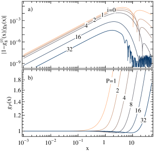
Figure 1: (a) Relative error in the estimates of $g_{8}(x)$ at different iterations of the self-consistent procedure in Eq. (17), with $\alpha=1/8$. The wiggles which appear after many iterations occur because each $g_{P}^{(i)}(x)$ is approximated as a spline interpolation before computing $g_{P}^{(i+1)}(x)$. These wiggles can be systematically reduced by using a denser grid in $x$. (b) Converged $g_{P}(x)$ curves for different bead numbers. Note that the curves with larger values of $P$ are flat up to larger values of $x$.

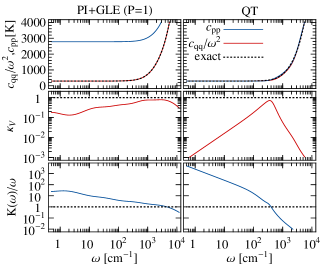
Figure 2: Comparison between the properties of the stochastic dynamics which result from the fitting strategy used in the present work (left column) and that used for the original quantum thermostatCeriotti, Bussi, and Parrinello (2009a) (right column), for simulations at $T=298$ K. Note that by sacrificing the fit to the fluctuations of momenta $[c_{pp}(\omega)]$ it is possible to obtain a perfect fit to $c_{qq}(\omega)$ and a better sampling efficiency $\kappa_{V}(\omega)=1/[\tau_{V}(\omega)\omega]$, where $\tau_{V}(\omega)$ is the correlation time of the potential energy for a harmonic oscillator with frequency $\omega$. In the case of PI+GLE it is less essential to enforce strong coupling to avoid zero point energy leakage, and it is therefore possible to avoid the overdamping which hinders the sampling in the case of the original quantum thermostat. This overdamping is clear from the bottom right-hand panel, which shows that $K(\omega)\gg\omega$ at low frequencies where $K(\omega)$ is the Fourier transform of the memory kernel in Eq. (9).

Before we describe our approach to solving Eq. (12), let us transform it into dimensionless form by defining $x=\hbar\omega/2k_{B}T$, $h(x)=x\coth x$, and $g_{P}(x)=(k_{B}T/P)(2x/\hbar)^{2}c_{qq}(2xk_{B}T/\hbar)$. With these definitions, Eq. (12) becomes

$$\sum_{k=0}^{P-1}\frac{g_{P}(x_{k})}{x_{k}^{2}/x^{2}}=h(x),$$ (13)

where

$$\quad x_{k}^{2}=x^{2}+P^{2}\sin^{2}\frac{k\pi}{P}.$$ (14)

The solution to Eq. (13) is not unique, and one must pick a particular solution by means of appropriate boundary conditions. In particular, one would like to enforce a physical behavior on the solution, with no discontinuities and reasonable asymptotic forms in the $x\rightarrow 0$ and $x\rightarrow\infty$ limits. The tentative solution

$$g^{(0)}_{P}(x)=h(x/P)$$ (15)

satisfies these requirements, and it is a good approximation to $g_{P}(x)$ from several points of view. First of all, it is the exact solution in the one-bead case (which corresponds to the bare quantum thermostat) and in the infinite bead limit, where it yields a constant effective temperature on all frequencies (which is correct, as in this case PIMD alone is sufficient to converge to the appropriate distribution). It also provides the appropriate large-$x$ limit for a smooth solution to Eq. (13), for arbitrary $P$.

In order to refine this tentative solution, one can cast Eq. (13) into a fixed-point iteration, by singling out the $k=0$ term:

$$g_{P}(x)=h(x)-\sum_{k=1}^{P-1}\frac{g_{P}(x_{k})}{x_{k}^{2}/x^{2}}.$$ (16)

We have found empirically that a self-consistent iterative procedure that yields an exact solution $g_{P}(x)$ to Eq. (13) to arbitrary precision can be obtained by stabilising Eq. (16) with a mixing strategy,

$$\begin{split}g_{P}^{(0)}(x)=&\ h(x/P)\\ g_{P}^{(i+1)}(x)=&\ \alpha\left[h(x)-\sum_{k=1}^{P-1}\frac{g_{P}^{(i)}(x_{k})}{x_{k}^{2}/x^{2}}\right]+(1-\alpha)g_{P}^{(i)}(x).\end{split}$$ (17)

In particular, the mixing parameter $\alpha=1/P$ was found to give a sufficiently fast and convergent iteration for all of the numbers of beads we tried. The convergence of $g_{P}^{(i)}(x)$ to $g_{P}(x)$ is shown in Fig. 1 for $P=8$, along with examples of the resulting converged solutions for other values of $P$. Tabulated values of these solutions for $P$ ranging from 1 to 128 can be downloaded from an on-line repositorygle . Once one has a converged $g_{P}(x)$, the frequency-dependent position fluctuation $c_{qq}(\omega)$ in Eq. (11) is given by

$$c_{qq}(\omega)=(Pk_{B}T/\omega^{2})g_{P}(\hbar\omega/2k_{B}T),$$ (18)

and the only remaining problem is to design a GLE that can be used to enforce this fluctuation on each ring polymer bead.

II.4 Fitting and implementation

The design of a GLE consistent with $c_{qq}(\omega)$ in Eq. (18) consists of optimising the matrices in Eq. (8) until the desired response of the thermostat is obtained. As has been found for a variety of other applications of the GLE,Ceriotti, Bussi, and Parrinello (2009b, a, 2010); Ceriotti et al. (2010a) the efficacy of the resulting PI+GLE scheme will depend on the strategy by which the optimisation is performed, and on the additional criteria besides fitting $c_{qq}(\omega)$ that are used to define the merit function for the optimisation. For applications of the quantum thermostat to anharmonic problems the strength of the coupling between the thermostat and the Hamiltonian dynamics and the efficiency of the sampling can be just as important as the agreement between $c_{qq}(\omega)$ and the target function in Eq. (18). The possibility of improving the accuracy systematically by increasing the number of beads makes zero-point energy leakage and other anharmonic effects a lesser concern in the present context. However, if systematic convergence is to be achieved, it is advisable that the sampling efficiency does not differ dramatically between the fits for different numbers of beads.

In the case of the original quantum thermostat described in Ref. Ceriotti, Bussi, and Parrinello (2009a), we chose to constrain $c_{pp}(\omega)=\omega^{2}c_{qq}(\omega)$ as in Eq. (10). This had the advantage of providing ready access to the quantum mechanical momentum distribution, which is a quantity of direct relevance to recent deep inelastic neutron scattering experiments. However, by constraining $c_{pp}(\omega)$ in this way, we found that we had to enforce a strongly overdamped regime at low frequencies in order to avoid zero point energy leakage in applications to multi-dimensional systems.Ceriotti, Bussi, and Parrinello (2009a) In the present PI+GLE scheme, as in PIMD itself, the ring polymer momenta lose all physical significance as soon as there is more than one bead, and extracting the quantum mechanical momentum distribution requires a considerably more intricate calculation.Lin et al. (2010) When it comes to fitting the GLE, it is therefore more natural to regard the momenta simply as a sampling device, and to focus exclusively on the fluctuations of configurations $c_{qq}(\omega)$, as we have already done in our description of PI+GLE in Sec. III.C.

As shown in Fig. 2, this leaves significantly more freedom in the fit, even in the case of just one bead. The extra freedom allows us to reproduce the desired $c_{qq}(\omega)$ with a maximum discrepancy smaller than $0.5$% and to achieve high sampling efficiency over a broad range of frequencies, yielding a sampling performance comparable to that of an “optimal sampling” GLE.Ceriotti, Bussi, and Parrinello (2010); Ceriotti et al. (2010a) To give another example involving more beads, the self-diffusion coefficient for a model of liquid water (see Sec. IV) - which in this context can only be regarded as a measure of the sampling efficiency for slow, collective motion - is reduced by less than 50% in a well-converged (8 bead) PI+GLE simulation compared to NVE dynamics, whereas the original (one bead) quantum thermostat decreases the diffusion coefficient of the same model by a factor of 10.

Having obtained a nearly-constant sampling efficiency is also beneficial to the transferability of the fitted parameters, as discussed in Refs.Ceriotti, Bussi, and Parrinello (2010); Ceriotti et al. (2010a). As a matter of fact, the very same parameterization has been adopted for both of the examples given below, which are as different as a one-dimensional quartic double well and liquid water. With an appropriate scaling,Ceriotti, Bussi, and Parrinello (2009a, 2010) these GLE parameters can be safely adopted in all circumstances where the maximum physical frequency present in the system is smaller than $35k_{B}T/\hbar$. The GLE parameters we have used in the present study are available up to $P=16$ and may be downloaded from an online repositorygle .

The details of how we actually optimised the GLE matrices for the present PI+GLE application are rather technical, and less important than the criteria employed for the optimisation that we have just described. A comprehensive discussion of the optimisation of GLE matrices has recently been given elsewhere,Ceriotti, Bussi, and Parrinello (2010) and we used exactly the same techniques in the present study. The implementation of a GLE thermostat into a PIMD code has also been discussed in detail in a recent paper,Ceriotti et al. (2010a) where it was shown to be essentially no more complicated than adding a thermostat to a classical molecular dynamics simulation. However, in the case of PI+GLE there are a few additional points that we do need to make.

First of all, the dynamics in PI+GLE must be performed using physical bead masses, as opposed to the alternative masses that are sometimes used in path integral schemes. Unless physical bead masses are used the frequencies of the necklace will be different from those in Eq. (5), and Eq. (14) will have to be modified accordingly; this will change the functional equation for $g_{P}(x)$ in Eq. (13) and the new equation will have to be solved from scratch. The equations of motion can be integrated efficiently with physical bead masses by performing a normal mode transformation for the free ring polymer evolutionCeriotti et al. (2010a) and/or employing a multiple time step scheme.Tuckerman, Berne, and Martyna (1992); Tuckerman et al. (1993)

Another important observation is that, at variance with canonical sampling GLE schemes in which the free particle propagation of the GLE preserves the equilibrium distribution, the stationary probability distribution of the PI+GLE scheme requires an accurate integration of the stochastic differential equations of motion on the timescale of the fastest modes. For this reason, whenever a multiple time step integrator is used, the thermostat should be applied in the inner loop. As a consequence, the integration of the GLE introduces a sizeable computational overhead, which can be significant in cases when the calculation of physical forces is inexpensive. In the case of ab initio molecular dynamics, which is the primary target for the present method, the overhead will be completely negligible.

III The quartic double well

As mentioned in the Introduction, one of the fundamental shortcomings of the original quantum thermostatCeriotti, Bussi, and Parrinello (2009a) is its inability to provide a realistic description of tunnelling effects. The one-dimensional double well potential,

$$V(q)=h\left[\left(\frac{2q}{d}\right)^{2}-1\right]^{2},$$ (19)

in which both zero-point energy and tunnelling are important, and can be tuned by adjusting the height $h$ of the barrier and the distance $d$ between the minima, therefore provides an ideal first example with which to benchmark the performance of our combined PI+GLE method.

In Fig. 3 we report the particle density $p(q)$ obtained in PIMD and PI+GLE simulations of this potential with $d=0.6$ Å and $h=1000$ K at a temperature of 300 K, using different numbers of beads. By comparing the curves with the exact finite-temperature density

$$\rho(q)=\sum_{i}e^{-\epsilon_{i}/k_{B}T}\left|\psi_{i}(q)\right|^{2}/\sum_{i}e^{-\epsilon_{i}/k_{B}T},$$ (20)

where $\epsilon_{i}$ and $\psi_{i}$ are the eigenvalues and eigenfunctions of the Schrödinger equation, one sees that the use of a GLE dramatically improves the results even when $P=1$. By increasing $P$ systematic convergence to exact result is achieved, and the convergence is greatly accelerated by the Langevin dynamics.

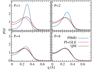
Figure 3: Probability density for a hydrogen atom in a quartic double well potential with the minima separated by $0.6$ Å and a barrier height of $1000$ K. All simulations were performed with a target temperature of $300$ K. The exact quantum mechanical result (dashed black line) was obtained by numerical solution of the Schrödinger equation, the contributions of the various eigenstates being averaged with the appropriate Boltzmann weight. The four panels compare this exact result with the PIMD and PI+GLE results with increasing bead numbers.

In order to characterise quantitatively the convergence of the density, we computed the distance between $p(q)$ and $\rho(q)$, as a function of the parameters of the potential and the bead number. For the distance metric we employed the square root of the Jensen-Shannon divergence

$$d^{2}_{JS}(p,\rho)=\frac{1}{2}\int_{-\infty}^{\infty}\left[p(q)\ln\frac{2p(q)}{p(q)+\rho(q)}+\ \rho(q)\ln\frac{2\rho(q)}{p(q)+\rho(q)}\right]dq,$$ (21)

which is a metric that is widely used to compare probability distributions.Endres and Schindelin (2003)

In Fig. 4 we present the convergence of $p(q)$ to $\rho(q)$ as the number of beads is increased. The simulations were performed using the mass of a hydrogen atom, different values of $d$ and $h$ as indicated in the figure, and a time step of $0.1$ fs. A very small time step was needed because we integrated the PI equations of motion directly using the velocity Verlet method, without exploiting the exact free ring polymer evolution that becomes possible in the normal mode representation.Ceriotti et al. (2010a) For each set of parameters we ran PIMD and PI-GLE trajectories for $20$ ns.

It is clear from Fig. 4 that the PI-GLE simulations yield a significantly better estimate of the finite-temperature density of the quartic double well than the PIMD simulations, even in the regime of small $d$ and large $h$ where tunnelling plays an important role. The addition of the GLE provides a given level of accuracy with an effort that is between two and eight times smaller than with a standard PI, depending on the parameters of the potential and on the accuracy required.

As the density approaches the exact $\rho(q)$, all physical observables that depend on the position of the particle converge to their quantum mechanical expectation values. In Fig. 5 we have plotted the average potential energy computed from the same trajectories that were used to compute the densities in Fig. 4. Again, the use of a GLE thermostat consistently improves the quality of results.

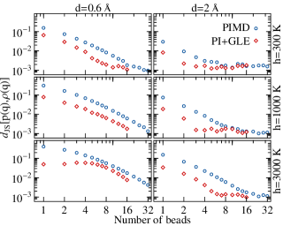
Figure 4: Distance between the exact density $\rho(q)$ and the densities $p(q)$ obtained from PIMD and PI+GLE simulations with different bead numbers, for the quartic double well potential in Eq. (19). Six different combinations of parameters of the double well potential have been tested. Note that in all cases the use of a GLE leads to a significant improvement in the estimate of the density.

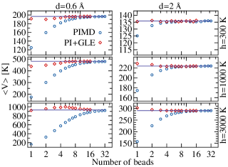
Figure 5: Average potential energy for a hydrogen atom in a quartic double well potential computed by PIMD and PI+GLE, as a function of the number of beads and for different parameters of the potential. The exact, quantum mechanical expectation value is marked with a line.

IV Liquid water

In the previous section we have demonstrated, in a simple one-dimensional case, that an appropriately-constructed GLE can be used to accelerate the convergence of path integral molecular dynamics to the exact quantum mechanical probability distribution. However, as discussed in earlier publications,Ceriotti, Bussi, and Parrinello (2009a, 2010) when applying the quantum thermostat to a multi-dimensional problem, one must be wary of zero point energy leakage. The GLE sets the various normal modes to different effective temperatures, and energy may flow from hot (high frequency) to cold (low frequency) modes because of anharmonic couplings.

To assess the behavior of the combined PI+GLE strategy in this respect, and to evaluate the computational savings that can be expected from the GLE in a more typical application, we have performed some additional simulations for liquid water. For these simulations, we used a recently-developed flexible water model that was fit to reproduce a wide variety of properties of the liquid in path integral simulations.Habershon, Markland, and Manolopoulos (2009) This avoids the double counting of nuclear quantum effects that would result from the use of a force field fit to reproduce experimental data in classical dynamics. We performed simulations with both conventional PIMD and PI+GLE, using different numbers of beads. The refined ring polymer contraction scheme of Markland et al.Markland and Manolopoulos (2008b) was used to reduce the computational effort, with the long-range electrostatic interactions beyond 5 Å contracted to the ring polymer centroid. The use of this scheme has been shown previously to provide significant computational savings in empirical force field simulations without affecting the accuracy of the results.Markland and Manolopoulos (2008b)

Simulations were performed with a target temperature $T=298$ K. We used a multiple-time step scheme with an outer time step of 0.75 fs and covalently bonded interactions computed every 0.15 fs. We ran 3.15 ns trajectories for each set of parameters, with the first 150 ps used for equilibration. Ergodic constant-temperature sampling was achieved in the PIMD simulations by applying a targeted stochastic scheme to the internal modes of the necklaceCeriotti et al. (2010a) and a global stochastic velocity rescaling to the centroid.Bussi, Donadio, and Parrinello (2007)

In Fig. 6 we report the expectation values of the potential energy and the centroid virial kinetic energy, which were computed using standard path integral estimators.Ceperley (1995) In this case, the GLE is seen to be extremely useful, and leads to much faster convergence of averages compared to conventional PIMD. Interestingly, we found that to converge average energies to an error smaller than $1$ kJ/mol in the PIMD simulations, $P$ should be increased well beyond the $32$ beads that are generally adopted for room-temperature water. Conversely, PI+GLE yields results in perfect agreement with a $128$ bead PIMD simulation using fewer than $16$ beads.

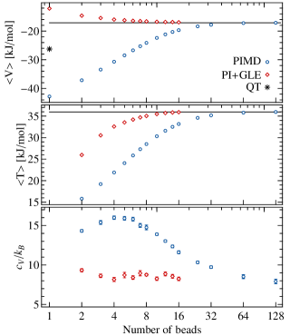
Figure 6: The average value of the potential energy and the virial kinetic energy for a simulation of a flexible water modelHabershon, Markland, and Manolopoulos (2009) at $T=298$ K, plotted as a function of the number of beads. The results obtained with conventional PIMD and PI+GLE are compared, and the value of $\left<V\right>$ obtained with the original quantum thermostatCeriotti, Bussi, and Parrinello (2009a) (QT) is also reported.

Figure 7: Errors in the radial distribution functions of liquid water at $T=298$ K obtained in low-$P$ simulations using PIMD and PI+GLE, relative to a fully-converged PIMD reference simulation with 128 beads. Note that the scale of the $y$-axis is greatly magnified as $P$ is increased and the $\Delta g$’s become smaller. The results obtained using the original quantum thermostatCeriotti, Bussi, and Parrinello (2009a) (QT) are also reported in the panels with $P=1$. The statistical error in the distribution functions is of the order of $10^{-3}$.

As a more sensitive benchmark of the convergence of the properties of quantum water we have also computed the constant-volume specific heat $c_{V}$, which is known to require very large values of $P$ for an accurate determination.Shiga and Shinoda (2005) The value of and statistical uncertainty in $c_{V}$ were obtained from a quadratic fit to the values of $\left<V\right>$ and $\left<T\right>$ computed at $293$, $298$ and $303$ K. The PI+GLE method is again seen to perform exceedingly well in this test (see Fig. 6). The convergence is somewhat accelerated by a fortuitous cancellation between the errors in the PI+GLE estimates of the potential and kinetic energy contributions to $c_{V}$, which are however both very well converged by the time $P\simeq 8$.

Comprehensive results for the convergence of structural properties of water are reported in Fig. 7, in which we systematically examine the radial distribution functions that are obtained with different bead numbers. Here again the GLE helps tremendously in accelerating the convergence of the PI calculation, in particular in the region of the intramolecular peaks, which are strongly affected by nuclear quantum effects. The only case in which the PI+GLE simulation is in worse agreement agreement with the exact result than the PIMD simulation is when the oxygen-oxygen $g(r)$ is computed with too few beads ($P=1$ and $P=2$). This is a consequence of the zero-point energy leakage in the PI+GLE simulation, which heats up low frequency degrees of freedom and washes out the long-range features from $g_{\rm OO}(r)$. By increasing the strength of the thermostat in the low-frequency region (as is done for instance in the case of the original quantum thermostat – see Sec. II.D) it is possible to mitigate this effect, at the expense however of a greater disturbance on diffusive modes, and hence on the efficiency of sampling. The PI+GLE strategy allows one to counter the effect of zero point energy leakage with a moderate increase in the number of beads, and indeed the PI+GLE radial distribution functions for liquid water are seen to be significantly more accurate than the PIMD radial distribution functions in Fig. 7 for all $P\geq 4$.

Combining the results in Figs. 6 and 7, one sees that PI+GLE provides the same accuracy in the thermodynamic and structural properties of liquid water with 8 beads as PIMD provides with 32 beads. This is the level of accuracy that is commonly accepted for room-temperature water simulations, and adding an appropriate GLE to the PI simulation allows it to be achieved with a four-fold reduction in the number of beads. The comparison becomes even more favourable if higher accuracy is required, with a 16-bead PI+GLE simulation being as accurate as a 128-bead PIMD simulation for all of the observables we have considered.

V Conclusions

In the present paper we have discussed and thoroughly demonstrated how a properly-designed generalized Langevin equation can be used to accelerate the convergence of path integral molecular dynamics to the exact quantum mechanical thermal expectation values. This leads to substantial savings in computational effort, the number of beads required to obtain a given level of accuracy being reduced by a factor of 4 or more. The original (one-bead) quantum thermostatCeriotti, Bussi, and Parrinello (2009a) provides an even cheaper way to include nuclear quantum effects in mildly anharmonic systems, but it is an inherently approximate technique. The present PI+GLE combination captures tunnelling effects as well as zero point energy effects, and it can be systematically improved to give the exact quantum mechanical result simply by increasing the number of path integral beads. We expect that this combination will be particularly valuable when used in conjunction with ab initio molecular dynamics, in which the forces acting on the nuclei are so expensive to evaluate that nuclear quantum effects have only seldom been considered in the past.

One final observation is that we have concentrated exclusively in this paper on the standard second order Trotter product path integral in Eqs. (3) and (4). Another way to reduce the number of path integral beads is to use a higher-order imaginary time propagator, and some interesting progress has been made in this direction over the years.Takahashi and Imada (1984); Chin (1997); Jang, Jang, and Voth (2001); Yamamoto (2005) This approach is fundamentally different from the approach we have investigated here, and potentially complementary to it. One could in principle develop a GLE scheme to accelerate the convergence of any imaginary time propagator, including the more promising of the higher-order propagators that have been suggested in the literature. In this way, one might hope to be able to reduce the number of beads even further, and make the inclusion of nuclear quantum effects in ab initio simulations almost routine. In any event, the results we have presented in this paper clearly demonstrate the potential of the generalized Langevin equation as a computational tool for accelerating the convergence of PIMD.

VI Acknowledgments

We would like to thank Oliver Riordan for a helpful discussion about the functional equation for $g_{P}(x)$ in Eq. (13) and the non-uniqueness of its solutions, and Giovanni Bussi and Thomas Markland for stimulating and insightful conversations.

References

- Morrone and Car (2008) J. A. Morrone and R. Car, Phys. Rev. Lett. 101, 017801 (2008).
- Chandler and Wolynes (1981) D. Chandler and P. G. Wolynes, J. Chem. Phys. 74, 4078 (1981).
- Feynman and Hibbs (1965) R. P. Feynman and A. R. Hibbs, Quantum Mechanics and Path Integrals (McGraw-Hill, New York, 1965).
- Markland and Manolopoulos (2008a) T. E. Markland and D. E. Manolopoulos, J. Chem. Phys. 129, 024105 (2008a).
- Markland and Manolopoulos (2008b) T. E. Markland and D. E. Manolopoulos, Chem. Phys. Lett. 464, 256 (2008b).
- Fanourgakis, Markland, and Manolopoulos (2009) G. S. Fanourgakis, T. E. Markland, and D. E. Manolopoulos, J. Chem. Phys. 131, 094102 (2009).
- Voth (1991) G. A. Voth, Phys. Rev. A 44, 5302 (1991).
- Ceriotti, Bussi, and Parrinello (2010) M. Ceriotti, G. Bussi, and M. Parrinello, J. Chem. Theory Comput. 6, 1170 (2010).
- Ceriotti et al. (2010a) M. Ceriotti, M. Parrinello, T. E. Markland, and D. E. Manolopoulos, J. Chem. Phys. 133, 124104 (2010a).
- Ceriotti, Bussi, and Parrinello (2009a) M. Ceriotti, G. Bussi, and M. Parrinello, Phys. Rev. Lett. 103, 030603 (2009a).
- Barker (1979) J. A. Barker, J. Chem. Phys. 70, 2914 (1979).
- (12) M. Parrinello and A. Rahman, in Monte Carlo Methods in Quantum Problems, edited by M. H. Kalos (Reidel, Dordrecht, 1984), page 105.
- Parrinello and Rahman (1984) M. Parrinello and A. Rahman, J. Chem. Phys. 80, 860 (1984).
- Ceperley (1995) D. M. Ceperley, Rev. Mod. Phys. 67, 279 (1995).
- Schulman (2005) L. S. Schulman, Techniques and Applications of Path Integration (Dover, New York, 2005).
- Cao and Voth (1994) J. Cao and G. A. Voth, J. Chem. Phys. 100, 5106 (1994).
- Jang and Voth (1999) S. Jang and G. A. Voth, J. Chem. Phys. 111, 2371 (1999).
- Craig and Manolopoulos (2004) I. R. Craig and D. E. Manolopoulos, J. Chem. Phys. 121, 3368 (2004).
- Braams and Manolopoulos (2006) B. J. Braams and D. E. Manolopoulos, J. Chem. Phys. 125, 124105 (2006).
- Zwanzig (2001) R. Zwanzig, Nonequilibrium Statistical Mechanics (Oxford University Press, Oxford, 2001).
- Gardiner (2003) C. W. Gardiner, Handbook of Stochastic Methods, 3rd ed. (Springer, Berlin, 2003).
- Habershon and Manolopoulos (2009) S. Habershon and D. E. Manolopoulos, J. Chem. Phys. 131, 244518 (2009).
- Khaliullin et al. (2010) R. Z. Khaliullin, H. Eshet, T. D. Kühne, J. Behler, and M. Parrinello, Phys. Rev. B 81, 100103 (2010).
- Ceriotti et al. (2010b) M. Ceriotti, G. Miceli, A. Pietropaolo, D. Colognesi, A. Nale, M. Catti, M. Bernasconi, and M. Parrinello, Phys. Rev. B 82, 174306 (2010b).
- (25) http://gle4md.berlios.de.
- Ceriotti, Bussi, and Parrinello (2009b) M. Ceriotti, G. Bussi, and M. Parrinello, Phys. Rev. Lett. 102, 020601 (2009b).
- Lin et al. (2010) L. Lin, J. A. Morrone, R. Car, and M. Parrinello, Phys. Rev. Lett. 105, 110602 (2010).
- Tuckerman, Berne, and Martyna (1992) M. E. Tuckerman, B. J. Berne, and G. J. Martyna, J. Chem. Phys. 97, 1990 (1992).
- Tuckerman et al. (1993) M. E. Tuckerman, B. J. Berne, G. J. Martyna, and M. L. Klein, J. Chem. Phys. 99, 2796 (1993).
- Endres and Schindelin (2003) D. M. Endres and J. E. Schindelin, IEEE Trans. Inf. Th. 49, 1858 (2003).
- Habershon, Markland, and Manolopoulos (2009) S. Habershon, T. E. Markland, and D. E. Manolopoulos, J. Chem. Phys. 131, 024501 (2009).
- Bussi, Donadio, and Parrinello (2007) G. Bussi, D. Donadio, and M. Parrinello, J. Chem. Phys. 126, 014101 (2007).
- Shiga and Shinoda (2005) M. Shiga and W. Shinoda, J. Chem. Phys. 123, 134502 (2005).
- Takahashi and Imada (1984) M. Takahashi and M. Imada, J. Phys. Soc. Japan 53, 3765 (1984).
- Chin (1997) S. A. Chin, Phys. Lett. A 226, 344 (1997).
- Jang, Jang, and Voth (2001) S. Jang, S. Jang, and G. A. Voth, J. Chem. Phys. 115, 7832 (2001).
- Yamamoto (2005) T. M. Yamamoto, J. Chem. Phys. 123, 104101 (2005).