A Comparative Note on Tunneling in AdS and
in its Boundary Matrix Dual

B. Chandrasekhar¹ , Sudipta Mukherji², Anurag Sahay² and Swarnendu Sarkar³

¹ Departamento de Fisica Mathematica, Universidad de Sao Paulo, Brazil 05315970

² Institute of Physics, Bhubaneswar-751 005, India

³ Department of Physics and Astrophysics, University of Delhi, Delhi 110007, India

Abstract

For charged black hole, within the grand canonical ensemble, the decay rate from thermal AdS to the black hole at a fixed high temperature increases with the chemical potential. We check that this feature is well captured by a phenomenological matrix model expected to describe its strongly coupled dual. This comparison is made by explicitly constructing the kink and bounce solutions around the de-confinement transition and evaluating the matrix model effective potential on the solutions.

1 Introduction and Summary

Quite a while back, Hawking and Page (HP) argued that at temperature below $T_{0}={\sqrt{2}}/(\pi l)$, thermal AdS background with a non-contractible Euclidean time circle $\beta=1/T$, is stable against collapse to form a black hole[1]. However, at a temperature higher than $T_{0}$, two Schwarzschild black holes nucleate, which following the literature, we call small and big black holes. While the small black hole is locally unstable, the other one has a positive specific heat. In fact, at a temperature $T$ greater than $T_{1}=3/(\pi l)>T_{0}$, the large black hole dominates the canonical ensemble for quantum gravity defined as a path integral over the metric and all other fields asymptotic to AdS with the periodicity of the time direction being $\beta$. It is believed that the small unstable black hole facilitates this transition. In the dual gauge theory, this represents a de-confining transition for ${\cal N}=4$, large $N$,  $SU(N)$ strongly coupled Yang-Mills on $S^{3}$. Though for gauge theory at finite coupling, there is no systematic way to compute an effective action, one may hope to construct a phenomenological model which captures this transition. Indeed in [2], partition function of YM theory was expressed as a matrix integral over the effective action involving Wilson-Polyakov loop. This model, which we review shortly, also predicts certain qualitative features that are not visible in the bulk supergravity approximation. Our aim in this paper is to put this matrix model to further qualitative checks. This is described in the following paragraph.

As we discussed in the beginning, HP transition is expected to be facilitated by the small unstable black hole. A particularly simple way to qualitatively analyze this transition would be to construct a bulk effective potential and to find instanton and bounce solutions at and above the HP temperature. In this regard, it turns out that the Bragg-Williams(BW) prescription is a particularly suitable framework (see [3] for details). In this approach, one constructs an approximate expression for the off-shell free energy function in terms of the order parameter and uses the condition that its equilibrium value minimizes the free energy. For describing HP transition from thermal AdS to the big black hole, horizon radius is an order parameter of the effective potential and the temperature then acts as an external tunable parameter. At the saddle point of this potential, however, the temperature gets related with the horizon radius in a way that is consistent with black hole thermodynamics. As we will describe shortly, following Coleman’s prescription [4], it is particularly simple to construct an exact instanton at HP temperature $T=T_{1}$ and the bounce above $T_{1}$ – a region where the big black hole becomes globally stable. Subsequently, one can compute the semi-classical decay rate from one phase to the other. Introduction of electrical charge into the system makes the chemical potential non-zero. The black hole in question is now the Reissner-Nordström black hole. In the grand canonical ensemble, as it was pointed out in [5], provided the chemical potential is less than a certain critical value, HP transition still persists. However, the critical temperature now gets a dependence on the chemical potential. It turns out that an appropriate BW potential can be constructed for which both temperature and chemical potential acts as independent tuning parameters. Exact instanton and the bounce solutions are easily computable. While computing these, we find that decay rate from AdS to the black holes phase, perhaps not surprisingly, increases with the chemical potential. Introduction of charge, in the boundary, is represented by turning on the R-charge of ${\cal N}=4$ SYM. As we discuss later, in the grand canonical ensemble, various qualitative features of this gauge theory with non-zero R-charge can still be incorporated into the earlier matrix model provided we make appropriate modifications. We find that the instanton and bounce solutions across the de-confining transition within this modified model can be semi-analytically calculated. Subsequently, our analysis also shows that, as expected from the bulk considerations, there is an enhancement of the decay rate with the chemical potential.

The paper is structured as follows. In the second section, we consider the gauge theory with zero chemical potential. In the bulk, we introduce the BW potential and discuss various kink and bounce solutions across the two phases and compute the decay rate. After a brief summary of the matrix model of [2], we then compute the kink, bounce solutions and decay rate around the de-confining transition. Section three addresses similar issues in the presence of a chemical potential in the grand canonical ensemble. Here we minimally modify the above matrix model to incorporate the effects due to the chemical potential. Once this is done, we go on to check other aspects of this model. In particular, we find that, as predicted from the bulk analysis, the decay rate from confining to the de-confining phase increases with the chemical potential.

2 Black hole and their matrix dual: zero chemical potential

In what follows, we first consider the gravity side, analytically compute instanton and bounce at and above the HP temperature. We use this to compute the value of the effective action on the solution. This provides us with the decay rate in the bulk. We then briefly review its phenomenological matrix dual and carry out similar computations across the de-confinement transition within this matrix model.

2.1 Bulk

For the Schwarzschild-AdS black holes, the BW potential is given by [3]

$${\cal F}(r,T)=E-TS=3(r^{2}+1)r^{2}-4\pi Tr^{3}.$$ (1)

Here $r$ measures the horizon size of the black hole, while $T,E,S$ are temperature, energy and entropy of the hole. Note that all the quantities are made dimensionless by multiplying them with appropriate powers of AdS radius $l$. $l$ does not appear explicitly as it has been set to $1$. Furthermore, we have set the Newton’s constant also to unity. $T$ in (1) should be understood as a tuning parameter whose dependence on $r$ follows from the on-shell equation

$$\frac{\partial{\cal F}}{\partial r}=0.$$ (2)

The thermal AdS potential can be obtained from (1) by setting $r=0$. Further, the first order transition arises when ${\cal F}=0$ and equation (2) is satisfied. The solution of these two equations are

$$r=1,~{}~{}~{}{\rm and}~{}~{}T_{1}=\frac{3}{2\pi}.$$ (3)

In figure (1 a), we have plotted (1) for various temperatures around the transition point. While stable minimum shown by the dotted line represents the stable big black hole for $T>T_{1}$, the stable minimum at $r=0$, shown in the dashed line, represents thermal AdS.

Following [4], we need to invert the potential, and, look for a kink solution connecting degenerate minima at $r=0$ and $r=1$ at $T=T_{1}$ shown by the solid line in (1 b). On the other hand, for $T>T_{1}$, we need to find the bounce solution connecting meta-stable and stable minima of the dotted line in (1 b).

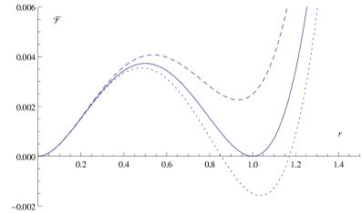
(a)

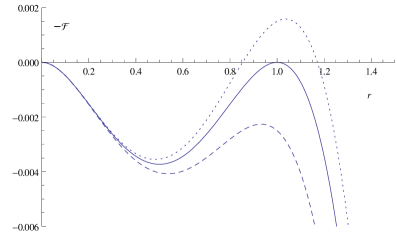
(b)

Figure 1: (a) This is ${\cal F}(r,T)$ plotted as a function of $r$. The dashed, solid and dotted lines are for $T<T_{1},T=T_{1}$ and $T>T_{1}$ respectively. (b) Inverse of the potential plotted as a function of $r$.

This is done by solving the equation

$$\frac{\partial r}{\partial\tau}={\sqrt{2{\cal F}(r,T)}},$$ (4)

where $\tau$ is the Euclidean time. This can be easily integrated with right boundary condition leading to the solution

$$r=\frac{6e^{\sqrt{3}\tau}}{1+4\pi Te^{\sqrt{3}\tau}+(4\pi^{2}T^{2}-9)e^{2\sqrt{3}\tau}}.$$ (5)

This solution is plotted in figure (2) for $T\geq T_{1}$. For $T=T_{1}$, it gives a kink solution connecting the minima at $r=0$ and $r=1$ representing the thermal AdS and the black hole phase. At a temperature above $T_{1}$, we get a bounce corresponding to the semi-classical tunneling from the metastable AdS phase to the stable black hole phase.

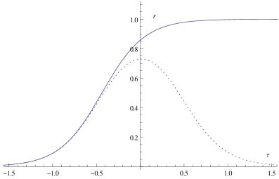
(a)

Figure 2: Figure shows the instanton and the bounce solutions. The solid line is for $T=T_{1}=3/(2\pi)$ and the dotted line is for $T=3.15/(2\pi)$ which is greater than the critical temperature.

It is straightforward to compute the Euclidean action on (5). We get

$$S_{E} =\int_{0}^{1}{\sqrt{{2\cal F}(r,T)}}dr$$ (6)

$$={\sqrt{2}}\Big{(}\frac{-9+6\pi^{2}T^{2}+\pi T(-9+4\pi^{2}T^{2})~{}{\rm log}~{}(3-2\pi T)}{9\sqrt{3}}$$

$$-\frac{1}{27}(-3+2\pi T)[3{\sqrt{6-4\pi T}}(2+\pi T)$$

$$+{\sqrt{3}}\pi T(3+2\pi T)~{}{\rm log}~{}(3-2\pi T+{\sqrt{6}}{\sqrt{3-2\pi T}})]\Big{)}.$$

For $T=T_{1}$, the Action evaluates to

$$S_{E}=\frac{1}{{\sqrt{6}}}.$$ (7)

The tunneling rate is therefore,

$$\Gamma\sim e^{-\frac{1}{\sqrt{6}\hbar}}.$$ (8)

2.2 Boundary

Having analyzed semi-classical decay of thermal AdS to a stable black hole at high temperature, we now turn our attention to the boundary dual. As mentioned previously, the framework within which we will search for similar kink and bounce solutions is the one proposed in [2] . It is a phenomenological model where partition function of YM theory was expressed as a matrix integral over the effective action involving Wilson-Polyakov loop $~{}({\rm tr}U)/N$. It contains two parameters $a$ and $b$ which, at fixed ’t Hooft coupling, depend on the temperature. The partition function is given by

$$Z(T)=\int dU\Big{[}a(T)~{}{\rm tr}U~{}{\rm tr}U^{\dagger}+\frac{b(T)}{N^{2}}(~{}{\rm tr}U~{}{\rm tr}U^{\dagger})^{2}\Big{]}.$$ (9)

This model was studied in some detail in the original paper [2] and was further reviewed in section 5 of [7]. We will be very brief here in describing the model. The effective potential arising from this model can be written in terms of $\rho=~{}{\rm tr}U~{}{\rm tr}U^{\dagger}/N^{2}$ as

$$V(\rho) =\frac{1-a}{2}\rho^{2}-\frac{b}{2}\rho^{4}\qquad{\rm for}~{}~{}0\leq\rho\leq\frac{1}{2}$$ (10)

$$=-\frac{a}{2}\rho^{2}-\frac{b}{2}\rho^{4}-\frac{1}{4}~{}{\rm log}~{}[2(1-\rho)]+\frac{1}{8}\quad{\rm for}~{}~{}\frac{1}{2}\leq\rho\leq 1.$$

The saddle point equation is given by

$$a\rho+b\rho^{3} =\rho~{}~{}{\rm for}~{}0\geq\rho\geq\frac{1}{2}$$ (11)

$$=\frac{1}{1-\rho}~{}~{}{\rm for}~{}\frac{1}{2}\geq\rho\geq 1.$$

The restrictions on $a$ and $b$ are $a<1,b>0$. We note that the comparison between this model and the bulk action is valid only when one neglects the string loop effects. The temperature at which the supergravity description breaks down is identified with the Gross-Witten transition in the matrix model.

The temperature dependence of the parameters can be fixed as follows. Let us consider a temperature $T>T_{0}$, $T_{0}$ being the black hole pair-nucleation temperature. At this temperature, we can write

$$2a\rho_{1,2}^{2}+2b\rho_{1,2}^{4}+~{}{\rm log}~{}(1-\rho_{1,2})+f=-I_{1,2},$$ (12)

where $I_{1,2}$ are the actions for the large and the small black holes. $\rho_{1,2}$ are the corresponding solutions in the matrix model. The constant $f=~{}{\rm log}~{}(2)-1/2$ is introduced to make the potential continuous at $\rho=1/2$. We further note that $\rho_{1,2}$ also have to satisfy the saddle point equations (11). These four equations uniquely determine $a,b$ and $\rho_{1,2}$ at a specific temperature. Further, continuing this process for various other temperatures, we get the dependence of temperature on $a(T)$ and $b(T)$. This can be done numerically and the result is shown is shown in figure (3).

Figure 3: Plots of $a(T,0)$ and $b(T,0)$. This is taken from [7]

We now proceed to look at instanton and bounce solution of this model. Though the method is same as the previous one, in order to proceed, we face a problem. The minimum at non-zero $\rho$ always appears in a region $\rho>1/2$. At the de-confining temperature $T=T_{1}=3/(2\pi)$ this minimum appears at $\rho=\rho_{1}=0.856,a=0.316,b=1.193$ and degenerates with the one at $\rho=0$ . So to get the complete instanton solution, we need to include integration of $V$ in (10) in the second region. However, because of the presence of the log term, we are unable to do an exact integration. In this region, we therefore resort to numerical method. In the region $0\leq\rho\leq 1/2$, the kink solution is given by

$$\rho(\tau)=\frac{4(1-a)e^{\sqrt{1-a}~{}\tau}}{4+b\,(1-a)\,e^{2\sqrt{1-a}~{}\tau}}~{}~{}~{}{\rm for}~{}0\leq\rho\leq\frac{1}{2},$$ (13)

for $a=0.316,b=1.193$. For the rest of the region, we numerically integrate the potential. The result is shown in figure (4).

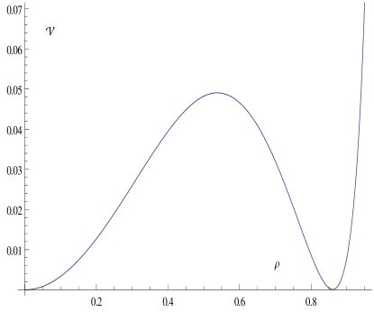
(a)

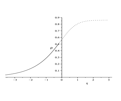
(b)

Figure 4: (a) $V(\rho)$ at $T=T_{1}$ for which $a=0.316,b=1.193$. Degenerate minima appear at $\rho=0$ and $\rho=0.856$. (b) Instanton connecting the minima.

For $T=T_{1}$, $a=0.316$ and $b=1.193$ the critical point is at $\rho=\rho_{0}=0.856$. Similar to the bulk case a calculation of the action for the instanton solution $\rho$ will give us the width of tunneling between the two solutions. A numerical integration of the instanton action evaluates to

$$\int^{\rho_{0}}_{0}\sqrt{2V(\rho)}d\rho=0.175$$ (14)

Hence the tunneling rate becomes

$$\Gamma=e^{-\frac{0.175}{\hbar}}.$$ (15)

For $T\geq T_{1}$ the $\rho=0$ solution becomes metastable and, similar to the bulk case, one obtain bounce solutions. This is shown in figure (5).

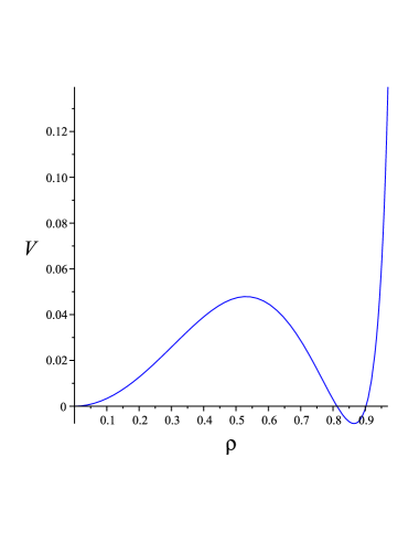
(a)

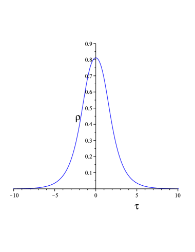
(b)

Figure 5: (a) This is $V(\rho)$ plotted as a function of $\rho$ for $T>T_{1}$, $a=0.316$ and $b=1.220$. (b) The bounce solution for the same potential with the turning point $\rho_{0}=0.810$

3 Black hole and their matrix dual: non-zero chemical potential

In this section, we will continue similar exploration in the presence of non-zero chemical potential. Our whole analysis will be carried in the grand canonical ensemble. We first study this problem in the bulk. In the boundary, we generalize the matrix model to include the effect of chemical potential. We then find the kink and bounces in this model. Calculating the decay rate from confining to the de-confining phase, we show that rate increases with the chemical potential. This is consistent with the expectation that arise from the bulk behavior.

3.1 Bulk

In the presence of electrical charge, we need to consider the Reissner-Nordström black holes. The BW free energy is easily computed and is given by [3]

$${\cal F}(r,T,\mu) = E-TS-Q\mu$$ (16)

$$= 3r^{2}(1-\frac{4}{3}\mu^{2})-4\pi r^{3}T+3r^{4}.$$

where $Q$ is the charge and $\mu$ is its conjugate chemical potential. We will restrict ourselves to the case where $\mu\leq{\sqrt{3}}/2$. At the saddle point,

$$r=\frac{3\pi T+{\sqrt{9\pi^{2}T^{2}-3(6-8\mu^{2})}}}{6}.$$ (17)

This can be inverted to get black hole temperature. While reducing the temperature below a critical value ($T_{1}$), this hole becomes globally unstable and system crosses over to the thermal AdS phase. This critical temperature depends upon the chemical potential and is given by

$$T_{1}=\frac{3{\sqrt{1-\frac{4}{3}\mu^{2}}}}{2\pi}.$$ (18)

As in the previous section, the kink solution within this effective description can be constructed at the critical temperature. It is given by

$$r(\tau)=\frac{2(3-4\mu^{2})e^{{\sqrt{3-4\mu^{2}}}~{}\tau}}{1+2{\sqrt{9-12\mu^{2}}}e^{{\sqrt{3-4\mu^{2}}}~{}\tau}}.$$ (19)

That the solution indeed interpolates between two phases, namely, the thermal AdS and the black hole, can be seen from the figure (6a). For $T>T_{1}$, the thermal AdS phase becomes metastable and we expect to find a bounce solution connecting this metastable phase to the stable one representing the black hole. Indeed this bounce can be explicitly constructed and is given by

$$r(\tau)=\frac{2(3-4\mu^{2})e^{{\sqrt{3-4\mu^{2}}}~{}\tau}}{1+4e^{{\sqrt{3-4\mu^{2}}}~{}\tau}\pi T+e^{2{\sqrt{3-4\mu^{2}}}~{}\tau}(12\mu^{2}+4\pi^{2}T^{2}-9)}.$$ (20)

This is plotted for different values of $\mu$ in (6b).

(a)

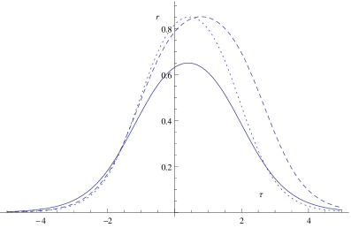
(b)

Figure 6: (a) Instanton solution at $T=T_{1}$ for $\mu=.5,.3$ and $.1$ are shown by solid, dashed and dotted lines respectively (b) Bounce solution for $T>T_{1}$ for different $\mu$. Solid, dashed and dotted lines are for $\mu=.5,.3$ and $.1$ at temperatures $.4,.45$ and $.48$ respectively. $T_{1}$ for these $\mu$ values are $0.390,0.447,0.474$ respectively.

It is straightforward to compute the Euclidean action on the instanton solution (19). We get

$$S_{E}=\int_{0}^{{\sqrt{1-\frac{4\mu^{2}}{3}}}}{\sqrt{2{\cal F}(r,T,\mu)}}$$

$$= \sqrt{2}(\frac{1}{27}(3\sqrt{3-4\mu^{2}}(-3+2\pi^{2}T^{2}+4\mu^{2})$$ (21)

$$+\sqrt{3}\pi T(-9+4\pi^{2}T^{2}12\mu^{2})Log[-2\pi T+\sqrt{9-12\mu^{2}}])$$

$$+(\sqrt{2}(-3+4\mu^{2})(-12\pi^{3}T^{3}+4\pi^{2}T^{2}\sqrt{9-12\mu^{2}}+15\pi T(3-4\mu^{2})$$

$$+6\sqrt{9-12\mu^{2}}(-3+4\mu^{2}))+\pi T\sqrt{9-12\mu^{2}}(9-4\pi^{2}T^{2}-12\mu^{2})\sqrt{9-12\mu^{2}-2\pi T\sqrt{9-12\mu^{2}}}$$

$$\log(-2\pi T+\sqrt{9-12\mu^{2}}+\sqrt{18-24\mu^{2}-4\pi T\sqrt{9-12\mu^{2}}}))$$

$$/(27\sqrt{\left(-3+4\mu^{2}\right)\left(-9+12\mu^{2}+2\pi T\sqrt{9-12\mu^{2}}\right)}))$$

At $T=T_{1}$ given in (18), we get

$$S_{E}=\frac{(3-4\mu^{2})^{\frac{3}{2}}}{9\sqrt{2}}$$ (22)

The tunneling rate is therefore,

$$\Gamma\sim e^{-\frac{(3-4\mu^{2})^{\frac{3}{2}}}{9\sqrt{2}\hbar}}$$ (23)

We see that decay rate increases with $\mu$.

3.2 Boundary

We now generalize the matrix model considered in the previous section to include the effect of the chemical potential. It turns out that minimal modification requires one to keep the structure of the potential same as (9), but to make $a$ and $b$ dependent on temperature as well as the chemical potential. One can now follow the same strategy as before to figure out the dependence of $a,b$ on $\mu$ and $T$. The only difference is that now in (12), we need to substitute $I_{1,2}$ for the Reissner-Nordström black hole. Carrying out the computation numerically we get $a,b$ as shown in the figure (7). A clear pattern that we see from here is that both these two parameters increase as we increase the chemical potential.

(a)

(b)

Figure 7: Plots show the behaviours of $a(\mu,T)$ and $b(\mu,T)$.

Once we have the data, we can go ahead and numerically compute the instanton, bounce and the decay rate. This is similar to the previous section with a little more complicacy due to non-zero $\mu$. We skip the details and show the results of our computation in the following figures.

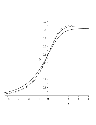
(a)

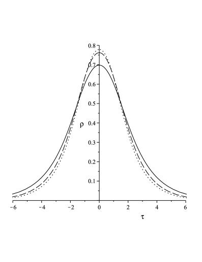
(b)

Figure 8: Boundary instanton and bounce curves. Compare with the previous figure (6) for the bulk case.(a) Solid, dashed and dotted curves correspond to instanton solutions for $(\mu,T_{1})=(0.5,0.390)\,(0.3,0.447)\,(0.1,0.474)$ respectively. (b) Bounce solutions at $T>T_{1}$ for different potentials. The solid, dashed and dotted curves correspond to $(\mu,T)=(0.5,0.4),\,(0.3,0.454),\,(0.1,0.48)$ respectively.

The effective action on the instanton solution can be evaluated numerically for this matrix model at different chemical potentials. The result is shown in figure (9). It is satisfying to find that, as in the bluk computation, the value of boundary effective action decreases with the increase of the chemical potential. This leads to an increase in the tunneling rate. We also note that the boundray dual is a phenomenonological model and is expected to capture only the qualitative features of the gravity dual. The functional forms of ${\cal F}(r)$ and $V(\rho)$ being different, it is not surprising that the two lines in figure (9) do not coincide.

In our study, we have adopted an effective approach towards the bulk gravity. Though this approach is particularly simple, enabling us to analytically construct kinks and bounce solutions, it would be instructive to directly analyze the gravitational bounce, compute the action against the bounce and then compare the results with the matrix model results. We leave this for our future study.

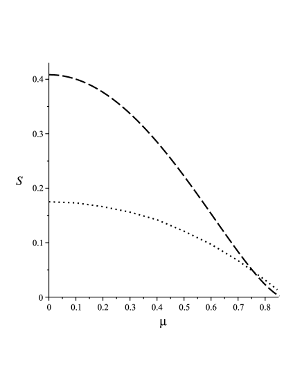
Figure 9: Behavior of effective matrix model potential calculated on the instanton is shown by the dotted line for different chemical potential. For comparison, the corresponding bulk action is also shown in the plot (dashed line). In both cases, actions decrease with $\mu$.

Acknowledgments: B.C. would like to thank Institute of Physics, Bhubaneswar for hospitality during the course of this work.

References

- [1] S. W. Hawking and D. N. Page, Commun. Math. Phys. 87, 577 (1983).
- [2] L. Alvarez-Gaume, C. Gomez, H. Liu, S. Wadia, Phys. Rev. D71, 124023 (2005). [hep-th/0502227].
- [3] S. Banerjee, S. K. Chakrabarti, S. Mukherji, B. Panda, Int. J. Mod. Phys. A26, 3469-3489 (2011). [arXiv:1012.3256 [hep-th]].
- [4] S. R. Coleman, Phys. Rev. D 15, 2929 (1977) [Erratum-ibid. D 16, 1248 (1977)].
- [5] A. Chamblin, R. Emparan, C. V. Johnson and R. C. Myers, Phys. Rev. D 60, 064018 (1999) [arXiv:hep-th/9902170].
- [6] P. Basu and S. R. Wadia, Phys. Rev. D 73, 045022 (2006) [arXiv:hep-th/0506203].
- [7] T. K. Dey, S. Mukherji, S. Mukhopadhyay, S. Sarkar, JHEP 0704, 014 (2007). [hep-th/0609038].
- [8] T. K. Dey, S. Mukherji, S. Mukhopadhyay, S. Sarkar, JHEP 0709, 026 (2007). [arXiv:0706.3996 [hep-th]].
- [9] T. K. Dey, S. Mukherji, S. Mukhopadhyay and S. Sarkar, Int. J. Mod. Phys. A 24, 5235 (2009) [arXiv:0806.4562 [hep-th]].