Constraints on quintessence and new physics from fundamental constants

Abstract

Changes in the values of the fundamental constants $\mu$, the proton to electron mass ratio, and $\alpha$, the fine structure constant due to rolling scalar fields have been discussed both in the context of cosmology and in new physics such as Super Symmetry (SUSY) models. This article examines the changes in these fundamental constants in a particular example of such fields, freezing and thawing slow roll quintessence. Constraints are placed on the product of a cosmological quantity, w, the equation of state parameter, and the square of the coupling constants for $\mu$ and $\alpha$ with the field, $\zeta_{x}$, ($x=\mu,\alpha$) using the existing observational limits on the values of $\frac{\Delta x}{x}$. Various examples of slow rolling quintessence models are used to further quantify the constraints. Some of the examples appear to be rejected by the existing data which strongly suggests that conformation to the values of the fundamental constants in the early universe is a standard test that should be applied to any cosmological model or suggested new physics.

1 Introduction

The values of the fundamental constants such as the fine structure constant $\alpha$ and the proton to electron mass ratio $\mu$ in the early universe provide important constraints and tests for cosmological theories such as quintessence and new physics models that suggest a coupling between the constants and rolling scalar fields. It was pointed out more than 35 years ago (Thompson, 1975) that changes in the value of the fundamental constant $\mu$ produce changes in molecular spectra such that observations of molecular spectra in high redshift objects can track the value of $\mu$ in the early universe. The recent advent of large telescopes with sensitive high resolution spectrometers and, most importantly, very accurate measurements of the wavelengths of the molecular hydrogen Lyman and Werner band transitions (Ubachs et al., 2007; Malec et al., 2010) have made such observations possible. Most of the relevant observations have been of the molecular hydrogen Lyman and Werner electronic absorption transitions in high redshift Damped Lyman Alpha systems (DLAs) (King et al., 2009; Wendt and Reimers, 2008; Thompson et al., 2009; Malec et al., 2010; King et al., 2011). These observations have restricted the change in $\mu$ to $\frac{\Delta\mu}{\mu}\leq 10^{-5}$ at redshifts up to 3. Radio observations have established limits on $\frac{\Delta\mu}{\mu}$ on the order of $10^{-6}$ using a comparison between the inversion transition of ammonia and the rotational transitions of other molecules at a redshift of 0.685 (Murphy et al., 2008) and at a redshift of 0.89 (Muller et al., 2011). At redshifts between 2 and 4 Curran et al. (2011) compared the frequencies of CO rotational lines to the frequency of the fine structure transition of neutral carbon. This comparison, however, does not measure $\mu$ directly but rather $F\equiv\frac{\alpha^{2}}{\mu}$. It is interesting, therefore, to see what constraints or limits these observations can put on cosmological models and the necessity of new physics not consistent with the standard model.

The situation regarding $\alpha$ is less clear given the conflicting claims on the variation (Murphy et al., 2004) or constancy (Chand et al., 2004) of $\alpha$ with even claims of a spatial dipole variation of $\alpha$ (Webb et al., 2011). Given this state of uncertainty we will concentrate mainly on the limits imposed by the constancy of $\mu$ but will also consider the consequences of a variation in $\alpha$ at the end of the analysis.

2 Cosmological Model

As a definite example of a cosmological model with a potential $V(\phi)$ defined by a rolling scalar field $\phi$ we will examine slow rolling freezing and thawing quintessence models following the discussion of Scherrer & Sen (2008) and Dutta & Scherrer (2011), hereinafter DS. In this case the dark energy is due to a minimally coupled scalar field $\phi$ governed by the equation of motion

$$\ddot{\Phi}+3H\dot{\phi}+\frac{dV}{d\phi}=0$$ (1)

where H is the Hubble parameter in units where $8\pi G=1$. The slow roll conditions are given by

$$\lambda^{2}\equiv(\frac{1}{V}\frac{dV}{d\phi})^{2}\ll 1$$ (2)

and

$$|\frac{1}{V}\frac{d^{2}V}{d\phi^{2}}|\ll 1$$ (3)

which leads to a very flat potential. Thawing solutions are where the equation of state parameter $w=p_{de}/\rho_{de}$ is initially near -1 and evolves away from -1 while freezing solutions start with $w$ not equal to -1 and evolve toward -1 at the present day. (DS) have shown that these cosmologies follow trajectories given by

$$1+w=\frac{1}{3}\lambda_{0}^{2}[\frac{1}{\sqrt{\Omega_{\phi}}}-(\frac{1}{\Omega_{\phi}}-1)(\tanh^{-1}(\sqrt{\Omega_{\phi}})+C)]^{2}$$ (4)

where C is determined by an early condition on $w$ and $\Omega_{\phi}$

$$C=\pm\frac{\sqrt{3(1+w_{i})}\Omega_{\phi_{i}}}{\lambda_{0}}$$ (5)

and the dark energy density factor $\Omega_{\phi}$ is given by

$$\Omega_{\phi}=[1+(\Omega_{\phi 0}^{-1}-1)a^{-3}]^{-1}$$ (6)

In (6) $a$ is the scale factor of the universe normalized to 1 at the present day and the subscript $0$ refers to the present epoch. Thawing solutions are given by the special case where $C=0$. The parameter $\lambda$ is necessarily small as given by equation 2 and is considered to be constant and equal to $\lambda_{0}$ at all times.

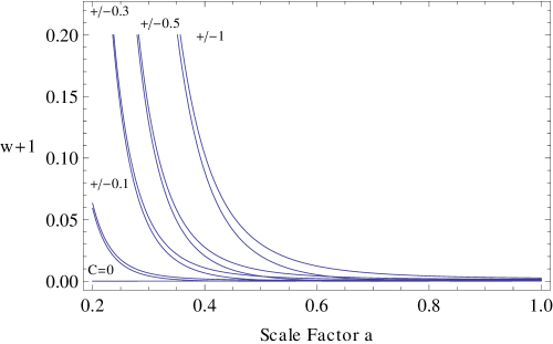
Figure 1: The evolution of w+1 as a function of the scale factor a for various values of C. The scale factor a is normalized to 1 at the present epoch. The track for C=0 is the thawing solution which starts near w+1=0 and ends with a value slightly larger than 0 at the present epoch. The values of $\lambda_{0}$ and $\Omega_{\phi i}$ are given in the last paragraph of section 2. Note that values of $1+w$ greater than 0.05 are beyond the range considered by DS.

(DS) consider several cases with values of C set to -1, -0.5, -0.1, 0., 0.1, 0.5, and 1 with $w_{i}=-0.95$, $\lambda_{0}=-0.08$, considered constant by DS, and $\Omega_{\phi i}$ adjusted to yield the listed values of C. We will use this suite of cases plus the added cases of C = -0.3 and C = 0.3 to determine what constraints are imposed by the observed values of $\mu$. Figure 1 shows the evolution of w+1 as a function of the scale factor a for the various values of C. Due to their large excursions from $w+1=0$ at high z the larger absolute values of C probably violate the slow roll condition. That is why we have added the C =+/-0.3 cases. All of the curves are for freezing quintessence except of the curve for C=0 which is for thawing quintessence. Although hard to see at the scale of Figure 1, the C=0 case for thawing quintessence has $w+1\neq 0$ at $a=1$.

3 New Physics and $\mu$

Since $\mu$ does not vary with time in the standard model any variation of $\mu$ must include new physics. This discussion follows the methodology described in Nunes & Lidsey (2004), hereinafter NL which presumes a linear, non-varying, coupling of $\mu$ to the rolling scalar field. There can be many variations of the coupling between $\mu$ and the scalar field but this represents one of the simplest models. (NL) actually consider the variation of the fine structure constant $\alpha$, however, most new physics models assume that $\alpha$ and $\mu$ vary in the same manner and are connected in the following manner

$$\frac{\dot{\mu}}{\mu}\sim\frac{\dot{\Lambda}_{QCD}}{\Lambda_{QCD}}-\frac{\dot{\nu}}{\nu}\sim R\frac{\dot{\alpha}}{\alpha}$$ (7)

eg. Avelino et al. (2006). In (7) $\Lambda_{QCD}$ is the QCD scale, $\nu$ is the Higgs vacuum expectation value and R is often considered to be on the order of -40 to -50 (Avelino et al., 2006) but it is highly indeterminate. The variation in $\alpha$ and consequentially $\mu$ is given as

$$\frac{\Delta\mu}{\mu}=R\zeta_{\alpha}\kappa(\phi-\phi_{0})=\zeta_{\mu}\kappa(\phi-\phi_{0})$$ (8)

where $\zeta_{x}$ ($x=\alpha,\mu$) is the coupling constant, $\kappa=\frac{\sqrt{8\pi}}{m_{p}}$ and $m_{p}$ is the Planck mass. Based on the work of Copeland et al. (2004) (NL) place limits on $|\zeta_{\alpha}|$ of $|\zeta_{\alpha}|\sim 10^{-4}-10^{-7}$ which translate to limits on $|\zeta_{\mu}|$ of $|\zeta_{\mu}|\sim 4\times 10^{-3}-4\times 10^{-6}$ for $R=-40$.

The equation of state is given in terms of the dark energy pressure $p_{\phi}$, dark energy density $\rho_{\phi}$ and dark energy potential $V(\phi)$ by

$$w\equiv\frac{p_{\phi}}{\rho_{\phi}}=\frac{\dot{\phi}^{2}-2V(\phi)}{\dot{\phi}^{2}+2V(\phi)}$$ (9)

(NL) then show that $w+1$ is also given by

$$w+1=\frac{(\kappa\phi^{\prime})^{2}}{3\Omega_{\phi}}$$ (10)

where $\Omega_{\phi}$ is the dark matter energy density. Here $\dot{\phi}$ and $\phi^{\prime}$ indicate differentiation with respect to cosmic time and to $N=\log{a}$ respectively where $a$ is again the scale factor. It follows from (8) that

$$\phi^{\prime}=\frac{\mu^{\prime}}{\kappa\zeta_{\mu}\mu}$$ (11)

Substitution of (11) into (10) then links $w$ and $\mu^{\prime}$ as

$$w+1=\frac{(\mu^{\prime}/\mu)^{2}}{3\zeta_{\mu}^{2}\Omega_{\phi}}=\frac{(\alpha^{\prime}/\alpha)^{2}}{3\zeta_{\alpha}^{2}\Omega_{\phi}}$$ (12)

which links the evolution of $w$, $\mu$ and $\alpha$.

4 Relating $\mu$, $\alpha$ and $w$

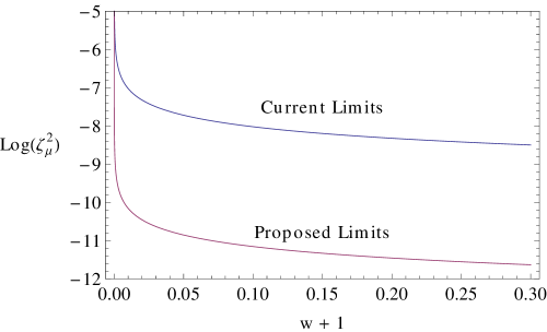
Figure 2: The parameter space in terms of $\log(\zeta_{\mu})^{2}$ and $(w+1)$ defined by the current limit on $\Delta\mu/\mu$ and for one that is 50 times lower than the present limit. All of the space above the two curves is forbidden in terms of the models and parameters presented here.

Now that we have two different equations for $w+1$, one involving only cosmological factors, the equation of state parameter, in the quintessence model discussed in section 2 and one involving new physics in section 3 we can see what constraints the observations place on the parameters for these models. From (12) we see that limits on $\Delta x/x$ place limits on the product $\zeta_{x}^{2}(w+1)$ if we assume that the cosmology of $\Omega_{\phi}$ is known from equation  6. Note that the use of equation  6 restricts the results to the slow roll conditions. Using the current limit on $\Delta\mu/\mu\leq 10^{-5}$ we can define regions of parameter space in a $(\zeta_{\mu})^{2}$ - $(w+1)$ landscape that are forbidden or allowed by those limits. Figure 2 shows that space for the current limit on $\Delta\mu/\mu$ and for one where the limit is 50 times more stringent, a possibility using observations from expected new spectrometers such as PEPSI on the LBT.

It is obvious that as $w+1$ approaches 0 that the constraint of $\zeta_{\mu}^{2}$ diminishes rapidly. This has to be so since it is the coupling with $\phi$ that both drives $w+1$ away from 0 and produces the change in $\mu$. If the improved limits are achieved then there will be a more than 1000 times stronger constraint on $\zeta_{\mu}^{2}$ even for very small values of $w+1$.

In the following we will use $\mu$ as a definite example but the result for $\alpha$ is exactly the same with $\zeta_{\alpha}$ replacing $\zeta_{\mu}$. Setting the right hand sides of equations  12 and  4 equal to each other we get

$$\frac{(\mu^{\prime}/\mu)^{2}}{3\zeta_{\mu}^{2}\Omega_{\phi}}=\frac{1}{3}\lambda_{0}^{2}\{\Omega_{\phi}^{-1/2}-(\Omega_{\phi}^{-1}-1)(\tanh^{-1}(\Omega_{\phi}^{1/2})+C)\}^{2}$$ (13)

which yields

$$\frac{\mu^{\prime}}{\mu}=\zeta_{\mu}\lambda_{0}\Omega_{\phi}^{1/2}\{\Omega_{\phi}^{-1/2}-(\Omega_{\phi}^{-1}-1)(\tanh^{-1}(\Omega_{\phi}^{1/2})+C)\}$$ (14)

We then use that $\mu^{\prime}=a(\frac{d\mu}{da})$ to produce

$$\frac{d\mu}{\mu}=\zeta_{\mu}\lambda_{0}\int_{1}^{a}\Omega_{\phi}^{1/2}\{\Omega_{\phi}^{-1/2}-(\Omega_{\phi}^{-1}-1)$$

$$\times(\tanh^{-1}(\Omega_{\phi}^{1/2})+C)\}a^{-1}da$$ (15)

$$\frac{d\mu}{\mu}=\zeta_{\mu}\lambda_{0}\int_{1}^{a}\{1-(\Omega_{\phi}^{-1/2}-\Omega_{\phi}^{1/2})$$

$$\times(\tanh^{-1}(\Omega_{\phi}^{1/2})+C)\}a^{-1}da$$ (16)

We next substitute in (6) for $\Omega_{\phi}$ to get

$$\frac{d\mu}{\mu}=\zeta_{\mu}\lambda_{0}\int_{1}^{a}\{1-[(1+(\Omega_{0}^{-1}-1)a^{-3})^{-1/2}$$

$$-(1+(\Omega_{0}^{-1}-1)a^{-3})^{1/2}]$$

$$\times[\tanh^{-1}(1+(\Omega_{0}^{-1}-1)a^{-3})^{1/2}+C]\}a^{-1}da$$ (17)

Since we know that $\mu$ is constant to one part in $10^{5}$ to observable limits we can treat $\mu$ in the denominator of the left side of (4) as a constant and finally get

$$\frac{\Delta\mu}{\mu}=\zeta_{\mu}\lambda_{0}\int_{1}^{a}\{1-[(1+(\Omega_{0}^{-1}-1)a^{-3})^{-1/2}$$

$$-(1+(\Omega_{0}^{-1}-1)a^{-3})^{1/2}]$$

$$\times[\tanh^{-1}(1+(\Omega_{0}^{-1}-1)a^{-3})^{1/2}+C]\}a^{-1}da$$ (18)

Equation 4 can be numerically integrated using Mathematica to show the evolution of the value of $\mu$ as a function of the scale factor a normalized to 1 at the present time and $\Omega_{0}$ set to 0.7. (DS) use a constant $\lambda$ of $\lambda_{0}=-0.08$, satisfying the first slow roll condition and consider a range of the constant $C$ between -1 and 1. Negative values of C correspond to a field rolling down the potential and positive values indicate the field initially rolling up the potential. (DS) indicate that the latter case is unlikely but they consider it for completeness. Figure 3 shows the results of the integration plotted as a function of redshift for a value of $\zeta_{\mu}=-4\times 10^{-4}$ which is consistent with $\zeta_{\alpha}=10^{-5}$ and $R=-40$.. It is evident from (4) that the results scale linearly with $\zeta_{\mu}$.

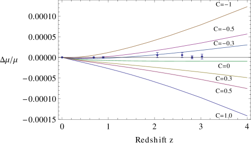
Figure 3: Plot of $\Delta\mu/\mu$ as a function of redshift $z=\frac{1}{a}-1$. The $C$ values are labeled in the figure and $\zeta{\mu}$ is set to $-4\times 10^{-4}$. All of the solutions are for freezing quintessence except for $C=0$ which is the thawing solution. The data points are taken from the information in Table 2 below along with the stated errors. The plotted points for objects with more than one reference are the most restrictive constraints. The erroneous Reinhold et al. (2006) and Ubachs et al. (2007) results are not shown.

A comparison of the observed value of $\Delta\mu/\mu$ and the $\Delta\mu/\mu$ values predicted by the models with $\zeta_{\mu}$ set to $-4.0\times 10^{-4}$ at a redshift of 3 is given in the first 7 entries of Table 1. It is evident from both the table and Figure 3 that most of the quintessence models considered in this paper, except for the thawing model, are ruled out by the observations if the coupling constant $\zeta_{\mu}$ is as high as $-4\times 10^{-4}$ and the magnitude of $C$ is significantly greater than 0. Since the value of $C$ sets the initial value of $w+1$ in the freezing models the small value of $\Delta\mu/\mu$ favors models where $w+1$ is small or 0 in the early universe. It is certainly possible to bring any of the quintessence models into compliance by lowering the value of either $\zeta_{\mu}$ or equivalently R in (7). However, these calculations show that using parameters that are common in the literature yields results that are incompatible with the present limits on $\Delta\mu/\mu$. It therefore suggests that the limits on the variance of fundamental constants is a rigorous test that should be applied to any proposed cosmological models or new physics. The slow roll conditions and the linear coupling of the fundamental constants with the field are conditions that provide a minimal change in the constants, therefore, these results impose an even stronger constraint on quintessence type models with much steeper potentials.

5 Imposing a condition on $\alpha$

There have been persistent claims in the literature that the value of $\alpha$ was different in the past than it is now. If we use the most recent claim of an altered previous value of $\alpha$ of $\Delta\alpha/\alpha=7\times 10^{-6}$ at redshifts around 3 (Webb et al., 2011) we can check what conditions this imposes on $\Delta\mu/\mu$. In Figure 4 we have adjusted $\zeta_{\alpha}$ to give a value of $\Delta\alpha/\alpha=7\times 10^{-6}$ for each value of C with R set to -40.

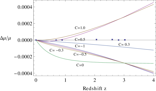
Figure 4: Plot of $\Delta\mu/\mu$ as a function of redshift with $\zeta_{\alpha}$ adjusted to give $\alpha$ of $\Delta\alpha/\alpha=7\times 10^{-6}$ at a redshift of 3. The $C$ values are labeled in the plot. Note that at z=1 the order of the plots is that C=-0.3 is the lowest and C=-1 is the highest of the three closely bunched solutions. The data points are the same as in figure 3.

It is clear from Figure 4 that none of the curves fit the high redshift $\Delta\mu/\mu$ measurements. Table 1 indicates that at a redshift of three the predictions differ from the observations by about a factor of 130. The thawing model ($C=0$) is a particularly bad fit even at low redshifts since $\zeta_{\alpha}$ has to be set to a very high value to achieve the claimed value of $\Delta\alpha/\alpha$. For this model the low redshift radio results of Murphy et al. (2008) are more than a factor of 1000 less than the predicted value. These results significantly increase the tension between the $\alpha$ and $\mu$ observations unless the magnitude of R in (7) is about -0.3 at an epoch when the redshift is about 3. This value of R is very different from the expected value of around -40 derived from generic GUT models where the strong coupling constant and the Higgs Vacuum Expectation Value run exponentially faster than $\alpha$ (Avelino et al., 2006). In this context either the expectations from Super Symmetry considerations are flawed or the conclusions from the observations indicating a change in the value of $\alpha$ in both space and time are in error.

$\frac{(\Delta\mu/\mu)_{0bs}}{(\Delta\mu/\mu)_{Mod}}$	$\zeta_{\mu}$	C
-0.022	$-4.0\times 10^{-4}$	-1.0
-0.039	$-4.0\times 10^{-4}$	-0.5
-0.059	$-4.0\times 10^{-4}$	-0.3
-0.23	$-4.0\times 10^{-4}$	0.0
-0.12	$-4.0\times 10^{-4}$	0.3
0.060	$-4.0\times 10^{-4}$	0.5
0.026	$-4.0\times 10^{-4}$	1.0
-0.0076	$-1.14\times 10^{-3}$	-1.0
-0.0076	$-2,08\times 10^{-3}$	-0.5
-0.0076	$-3.1\times 10^{-3}$	-0.3
-0.0076	$-1.2\times 10^{-2}$	0.0
0.0076	$-6.5\times 10^{-4}$	0.3
0.0075	$-3.2\times 10^{-3}$	0.5
0.0076	$-1.4\times 10^{-3}$	1.0

Table 1: Model Predictions versus Observations at Z=3. The first 7 entries are for $\zeta_{\mu}$ held at $-4.0\times 10^{-4}$. In the last 7 entries the value of $\zeta_{\mu}$ is adjusted to produce a $\Delta\alpha/\alpha$ value of $7\times 10^{-6}$ with R held at -40.

Conclusions

Constraints on the values of the fundamental constants $\mu$ and $\alpha$ now impose meaningful constraints on both cosmological models and new physics in terms of the product of the equation of state parameter $(w+1)$ and a new physics term $\zeta_{x}^{2}$ ($x=\mu,\alpha$) as shown in figure 2. Given a specific cosmological model such as slow roll quintessence and expected parameters for the coupling constants $\zeta_{x}$ predictions of the changes in the fundamental constants $\Delta x/x$ can be made. These predictions, using parameters common in the literature, are discrepant with the observational constraints at high redshift by up to two orders of magnitude for some cases. This argues for the inclusion of the values of the fundamental constants in the early universe into the commonly accepted tests for either cosmological models or new physics. It is certainly true that the new physics and cosmological parameters can be adjusted to satisfy the fundamental constant constraints. The main point, however, is that the parameters are no longer completely free but must be contained within observational bounds. Improvements in the measurement of the fundamental constants can significantly improve the constraints and provide even more stringent bounds on new physics and cosmology. An improvement by a factor of 50 on the current constraint on $\Delta\mu/\mu$ of $\leq 10^{-5}$ produces more than a thousand fold improvement of the constraint on $(\zeta_{\mu})^{2}(w+1)$. Such an improvement should be possible with new instrumentation such as the PEPSI spectrometer on the Large Binocular Telescope.

Appendix A Current determinations of $\Delta\mu/\mu$

Table 2 lists the current determinations of $\Delta\mu/\mu$ in distant galaxies and in the Milky Way. A subset of the most recent constraints are used in figures 3 and 4. In particular the erroneous positive results of Reinhold et al. (2006) have not been included.

Object	Reference	Redshift	$\Delta\mu/\mu$
Q0347-383	Wendt and Reimers (2008)	3.0249	$(2.1\pm 6)\times 10^{-6}$
Q0347-383	King et al. (2009)	3.0249	$(8.2\pm 7.4)\times 10^{-6}$
Q0347-383	Thompson et al. (2009)	3.0249	$(-2.8\pm 1.6)\times 10^{-5}$
Q0528-250	King et al. (2009)	2.811	$(1.4\pm 3.9)\times 10^{-6}$
Q0528-250	King et al. (2011)	2.811	$(0.3\pm 3.7)\times 10^{-6}$
Q0405-443	Thompson et al. (2009)	2.5974	$(3.7\pm 14)\times 10^{-6}$
Q0405-443	King et al. (2009)	2.5974	$(10.1\pm 6.2)\times 10^{-6}$
J2123-005	Malec et al. (2010)	2.059	$5.6\pm 6.2)\times 10^{-6}$
PKS 1830-211	Muller et al. (2011)	0.89	$\leq 2.\times 10^{-6}$
B0218+357	Murphy et al. (2008)	0.6847	$\leq 0.18\times 10^{-6}$
Milky Way	Molaro et al. (2009)	0.0	$(4-14)\times 10^{-8}$

Table 2: Recent Astronomical $\Delta\mu/\mu$ Measurements

References

- Avelino et al. (2006) Avelino, P.P, Martins, C.J.A.P., Nunes, N.J. & Olive, K.A. 2006, Phys. Rev. D., 74, 083508
- Chand et al. (2004) Chand, H., Srianand, R., Petitjean, P., and Aracil, B.. 2004, A&A 417, 853
- Copeland et al. (2004) Copeland, E.J., Nunes, N.J. & Pospelov, M. 2004, Phys. Rev. D, 69, 023501
- Curran et al. (2011) Curran, S.J. et al. 2011, AAP, 533, A55
- Dutta & Scherrer (2011) Dutta, S. & Scherrer, R.J. 2011, Physics Letters B, Volume 704, Issue 4, p. 265-269.
- King et al. (2009) King, J. A., Webb, J. K., Murphy, M. T. & Carswell, R. F. 2009, PRL, 101, 251304
- King et al. (2011) King, J. A., Webb, J. K., Murphy, M., Ubachs, W, & Webb, J. 2011, MNRAS, 417, 3010
- Malec et al. (2010) Malec, A.L. et al. 2010, MNRAS, 403, 1541
- Molaro et al. (2009) Molaro, P., Levshakov, S.S. & Kzolov, M.G. 2009, Nuc. Phys. B Proc. Supp., 194, 287
- Muller et al. (2011) Muller, S. et al. 2011, arXiv:1104.3361v1
- Murphy et al. (2004) Murphy, M.T., Webb, J.K. & Flambaum, V.V. 2004, MNRAS, 345, 609
- Murphy et al. (2008) Murphy, M.T., Flambaum, V.V., Muller, S., & Henkel, C. 2008, Science, 320, 1611
- Nunes & Lidsey (2004) Nunes, N.J. & Lidsey, J.E. 2004, Phys Rev D, 69, 123511
- Reinhold et al. (2006) Reinhold, E. et al. 2006, Phys. Rev. Lett., 96, 151101.
- Scherrer & Sen (2008) Scherrer, R.J. & Sen, A.A. 2008, Phys. Rev. D, 77, 083515
- Thompson (1975) Thompson, R.I., 1975, Astrophysical Letters, 16, 3
- Thompson et al. (2009) Thompson, R.I. et al. 2009, Ap.J., 703, 1648
- Ubachs et al. (2007) Ubachs, W., Buning, R., Eikema, K.S.E. & Reinhold,E., 2007, Journal of Molecular Spectroscopy, 241, 155
- Wendt and Reimers (2008) Wendt, M. & Reimers, D. 2008, Eur. Phys. J. ST, 163, 197
- Webb et al. (2011) Webb, J.K., King, J.A., Murphy, M.T., Flambaum, V.V., Darswell, R.F., & Bainbridge, M.B. 2011, PRL, 107, 191101-1-5