February 2012
ITP-UU-12/06
SPIN-12/05

Abstract

The hybrid NLIE of AdS${}_{5}\times{}$S⁵ is applied to a wider class of states. We find that the Konishi state of the orbifold AdS${}_{5}\times{}$S${}^{5}/\mathbb{Z}_{S}$ satisfies $A_{1}$ NLIE with the source terms which are derived from contour deformation trick. For general states, we construct a deformed contour with which the contour deformation trick yields the correct source terms.

1 Introduction and Summary

The primary example of AdS/CFT correspondence is the one between four-dimensional ${\mathcal{N}}=4$ super Yang-Mills and AdS${}_{5}\times{}$S⁵ string theory [1]. The spectrum of string states on AdS${}_{5}\times{}$S⁵ can be computed by the mirror Thermodynamic Bethe Ansatz (TBA) equations [2, 3, 4] based on string hypothesis in the mirror model [5, 6]; or equivalently the extended Y-system on $\mathfrak{psu}(2,2|4)$-hook [7, 8, 9]. It is believed that these methods give the exact answer, because they capture all finite-size corrections [10, 11].

The numerical study of the mirror TBA has made progress [12, 13, 14, 15]. However, it suffers from the problem of critical coupling constants [16]. The analyticity of the unknown variables called Y-functions changes around certain values of ’t Hooft coupling constant, and the explicit form of the TBA equations changes there discontinuously. As a result, it is difficult to solve the equation with high precision around the critical values, and to judge if the exact energy does not show unusual behavior like inflection points around the critical points.

The author has recently applied the method of hybrid nonlinear integral equations (hybrid NLIE) [17] to the mirror TBA for AdS${}_{5}\times{}$S⁵ [18]. This method replaces the horizontal part of the mirror TBA equations by $A_{1}$ NLIE. The hybrid NLIE consists of a smaller set of unknown variables than the mirror TBA, and we expect that it suffers less often from the problem of critical coupling constants. We exemplify our expectation in a way similar to [16].

For this purpose the mirror TBA for the twisted AdS${}_{5}\times{}$S⁵ offers a desired playground, because all Y-functions have intricate analytic properties, depending on the twist angle $\alpha$ and ’t Hooft coupling constant $g=\frac{\sqrt{\lambda}}{2\pi}$. The orbifold Konishi state is the simplest nontrivial example that exhibits critical behavior in the mirror TBA for $Y_{M|w}$. For this state, we find that the hybrid NLIE also exhibits critical behavior; its source terms change discontinuously across certain values of coupling constant.

Orbifold Konishi is a two-particle state in the $\mathfrak{sl}(2)$ sector of AdS${}_{5}\times{}$S${}^{5}/\mathbb{Z}_{S}$, where the $\mathbb{Z}_{S}$ acts on $\mathfrak{su}(2)^{2}\subset[\mathfrak{su}(2|2)^{2}\cap\mathfrak{su}(4)]$. This is also a special state in the twisted AdS${}_{5}\times{}$S⁵, $\beta$- or $\gamma$-deformed AdS${}_{5}\times{}$S⁵ models. The orbifold and $\gamma$-deformed models are another important examples of AdS/CFT correspondence, realized in gauge theory [24, 25, 26, 27, 28, 29, 30] and in string theory [31, 32, 33, 34, 35]. Finite-size corrections of deformed theories have been studied in gauge theory [36, 37, 38], in string theory [39], by Lüscher formula [40, 41, 42, 43, 44, 45, 46, 47], and by the mirror TBA or Y-system [48, 49, 50, 51, 52]. However, it is not clear if the corresponding sigma model on twisted AdS${}_{5}\times{}$S⁵ possesses integrability (see [53] for review), though integrable twists exist mathematically.

Next, we notice that such discontinuous change of the NLIE for the orbifold Konishi state can be explained by the contour deformation trick. There is a conjecture that the TBA for excited states follows from the TBA for the ground state by analytic continuation of coupling constant [54, 55]. It is expected that such analytic continuation introduces extra singularities of the integrand on the complex rapidity plane, and deforms the integration contour accordingly. Then, the excited states TBA should be expressed equivalently either as the ground-state TBA integrated over the deformed contour, or as the TBA integrated over the real line with additional source terms. This idea is called contour deformation trick. The contour deformation trick predicts how to correct the TBA when numerical iteration ceases to converge due to the change of analyticity, and is a guideline to study various states in the mirror TBA [16] including boundstates [56]. The $A_{1}$ NLIE with source terms has been studied in various examples [57, 58, 59, 60, 61, 62, 63, 64, 65], and the contour deformation trick was used in [66, 67].

With successful examples of the contour deformation in mind, we ask what the most general possible source terms are, and if they are obtained by the contour deformation trick. In principle, $A_{1}$ NLIE can be derived even when the Q-functions are meromorphic, rather than analytic, in the upper or lower half plane. Then the isolated singularities of Q-functions provide extra source terms to $A_{1}$ NLIE. It is a nontrivial question whether such source terms can be explained by the contour deformation trick, particularly with the same contour as in the orbifold Konishi state. Indeed, mismatch is found between the two results. To reconcile this problem, we construct a deformed contour which is consistent for general states including orbifold Konishi. The consistent deformed contour picks up only the preferred singularities of the integrand and runs both the lower and upper half planes. The details will be discussed in Section 3.

The contour deformation trick illustrates the difference between hybrid NLIE and FiNLIE [68]. In the latter the integrals run over the gap discontinuity of dynamical variables, which is not something to be deformed. In contrast, hybrid NLIE is written in terms of gauge-invariant (but frame-dependent) variables, allowing us to handle the equations similar to that of the mirror TBA.

This paper is organized as follows. In Section 2, we study the orbifold Konishi state from the mirror TBA and hybrid NLIE, and clarify the critical behavior in the asymptotic limit. In Section 3, we discuss the source terms of $A_{1}$ NLIE in view of contour deformation trick. Section 4 is for conclusion. In appendices, we introduce our notation, review the NLIE variables, compute the asymptotic transfer matrix in the form of Wronskian, and derive the results in Section 3.

2 TBA and NLIE for twisted AdS${}_{5}\times{}$S⁵

We study the critical behavior of hybrid NLIE for the orbifold Konishi state as a specific example. We briefly review the mirror TBA in twisted AdS${}_{5}\times{}$S⁵ and their critical behavior.

2.1 Orbifold Konishi state

The orbifold Konishi state can be defined in two equivalent ways.

The first is to consider the $\mathfrak{sl}(2)$ Konishi descendant on the orbifold AdS${}_{5}\times{}$S${}^{5}/\mathbb{Z}_{S}$, where the $\mathbb{Z}_{S}$ action is chosen as follows (see [49]). We decompose the transverse 8+8 fields of AdS${}_{5}\times{}$S⁵ into $({\bf 2}|{\bf 2})\otimes({\bf 2}|{\bf 2})$ representation of $\mathfrak{su}(2|2)_{L}\times\mathfrak{su}(2|2)_{R}$ , as

$$\left(\Phi^{I}\,,D_{\mu}Z\,,\Psi\,,\overline{\Psi}\right)\quad\leftrightarrow\quad\left(Y_{b\dot{b}}\,,Y_{\beta\dot{\beta}}\,,Y_{b\dot{\beta}}\,,Y_{\beta\dot{b}}\right)\equiv(y_{b}\,y_{\dot{b}}\,,\eta_{\beta}\,\eta_{\dot{\beta}}\,,y_{b}\,\eta_{\dot{\beta}}\,,\eta_{\beta}\,y_{\dot{b}}),$$ (2.1)

where $b,\dot{b}=1,2$ refer to the ${\rm S}^{5}$ part, and $\beta,\dot{\beta}=3,4$ refer to the ${\rm AdS}_{5}$ part of $\mathfrak{su}(2|2)^{2}$. The boundary conditions of $y_{b}$ are twisted by $\mathbb{Z}_{S}$ as

$$\begin{pmatrix}y_{1}(\sigma=2\pi)\\ y_{2}(\sigma=2\pi)\end{pmatrix}=\begin{pmatrix}e^{+i\alpha_{L}}&0\\ 0&e^{-i\alpha_{L}}\end{pmatrix}\begin{pmatrix}y_{1}(\sigma=0)\\ y_{2}(\sigma=0)\end{pmatrix},\qquad\alpha_{L}=\frac{2\pi n_{L}}{S}\quad(n_{L}\in\mathbb{Z}).$$ (2.2)

Similarly, the boundary conditions of $y_{\dot{b}}$ are twisted by $\alpha_{R}=\frac{2\pi n_{R}}{S}$ . The orbifold action $\left({\rm\ref{def:ZS action}}\right)$ affects only the auxiliary part of the asymptotic Bethe Ansatz equations. Thus, if we set the total momentum to zero as in the ordinary Konishi state, the asymptotic Bethe roots remain unchanged before and after orbifolding. This is called orbifold Konishi state.

The second is to introduce integrable twisted boundary conditions to the transfer matrix of AdS${}_{5}\times{}$S⁵. To preserve the integrability, the twist operator must commute with the S-matrix. When the twist operator belongs to $[\mathfrak{su}(2|2)^{2}\cap\mathfrak{su}(4)]$ and the twist angle is equal to a multiple of $2\pi/S$, Konishi state of the twisted AdS${}_{5}\times{}$S⁵ is equivalent to the orbifold Konishi state.

The second point of view is useful to construct the twisted transfer matrix, as defined by

$$T_{Q,1}^{L}={\rm str}_{Q}\left[g_{0}\,\mathbb{S}_{01}\,\mathbb{S}_{02}\,\dots\,\mathbb{S}_{0N}\right],\qquad g_{0}={\rm diag}\left(e^{+i\alpha_{L}}\,,e^{-i\alpha_{L}}\,,1,1\right).$$ (2.3)

and similarly for $T_{Q,1}^{R}$. The $\mathbb{S}_{0i}$ is the S-matrix between the mirror particle and the $i$-th particle in string theory. We can diagonalize $\left({\rm\ref{def:twisted transfer L}}\right)$ by algebraic Bethe Ansatz [69]. In practice, it is easier to twist the generating function for the eigenvalues of transfer matrices [70, 49, 48]. This construction will be discussed in Appendix C, where we also rewrite the transfer matrices in the form of Wronskian. In what follows we set $\alpha_{L}=\alpha_{R}\equiv\alpha$ for simplicity.

The mirror TBA for the twisted model is obtained as follows. The twist angle $\alpha$ in string theory corresponds to the insertion of defect operator in mirror theory [46]. In particular, the same mirror string hypothesis is used in both twisted and untwisted models. In the case of orbifold, the defect operator can be identified as an extra chemical potential, and it changes the $v\to\pm\infty$ asymptotics of Y-functions [50]. The mirror TBA equations for twisted AdS${}_{5}\times{}$S⁵ are solved by the twisted transfer matrices in the asymptotic limit [49].

2.2 TBA and NLIE in horizontal strips

We compare mirror TBA and hybrid NLIE in the horizontal part of the $\mathfrak{psu}(2,2|4)$-hook for the twisted AdS${}_{5}\times{}$S⁵. We will consider only the states which are invariant under the interchange $(a,s)\to(a,-s)$ of the $\mathfrak{psu}(2,2|4)$-hook.

The simplified TBA equation for $Y_{1|w}$ and $Y_{M|w}\ (M\geq 2)$ can be written as

$$\log Y_{1|w} =-V_{1|w}+\log(1+Y_{2|w})\star s_{K}+\log\frac{1-\frac{1}{Y_{-}}}{1-\frac{1}{Y_{+}}}\,\hat{\star}\,s_{K}\,,$$ (2.4)

$$\log Y_{M|w} =-V_{M|w}+\log(1+Y_{M+1|w})\star s_{K}+\log(1+Y_{M-1|w})\star s_{K}\,,$$ (2.5)

where $V_{M|w}$ is the source term, which depends on the state and the values of $(\alpha,g)$ under consideration. In the hybrid NLIE, the $1+Y_{M+1|w}$ on the right hand side is replaced by

$$1+Y_{2|w}=(1+\mathfrak{a}_{3}^{\nu\,[+\gamma]})\,(1+\overline{\mathfrak{a}}_{3}^{\nu\,[-\gamma]}),\qquad 1+Y_{M+1|w}=(1+\mathfrak{a}_{M+2}^{\nu\,[+\gamma]})\,(1+\overline{\mathfrak{a}}_{M+2}^{\nu\,[-\gamma]}).$$

The pair of parameters $\left\{\mathfrak{a}_{s}^{\nu}\,,\overline{\mathfrak{a}}_{s}^{\nu}\right\}(s\geq 3)$ are determined by $A_{1}$ NLIE,

$$\log\mathfrak{a}_{s}^{\nu} =-J_{s}^{\nu}+\log(1+\mathfrak{a}_{s}^{\nu})\star K_{f}-\log(1+\overline{\mathfrak{a}}_{s}^{\nu})\star K_{f}^{[+2-2\gamma]}+\log(1+Y_{s-2|w})\star s_{K}^{[-\gamma]}\,,$$ (2.6)

$$\log\overline{\mathfrak{a}}_{s}^{\nu} =-\overline{J}_{s}^{\nu}+\log(1+\overline{\mathfrak{a}}_{s}^{\nu})\star K_{f}-\log(1+\mathfrak{a}_{s}^{\nu})\star K_{f}^{[-2+2\gamma]}+\log(1+Y_{s-2|w})\star s_{K}^{[+\gamma]}\,,$$ (2.7)

where $\nu={\rm I}$ or ${\rm II}$ refers to the two sets of Q-functions [18], and $\gamma\ (0<\gamma<1)$ is a regularization parameter, as reviewed in appendix B. We leave $s\in\mathbb{Z}_{\geq 3}$ unspecified, though one can substitute $s=3$ at any time. The case of $\nu={\rm I}$ is simpler than $\nu={\rm II}$, because the source terms $\{J_{3}^{\rm I}\,,\overline{J}_{3}^{\rm I}\}$ vanishes in the Konishi state of the untwisted AdS${}_{5}\times{}$S⁵ model, at least asymptotically. Below we consider the case $\mathfrak{a}_{s}^{\rm I}\,,\overline{\mathfrak{a}}_{s}^{\rm I}$ only, and omit $\nu={\rm I}$. In short, the $Y_{M|w}$ functions of the mirror TBA are replaced by three dynamical variables, $(\mathfrak{a}_{3}\,,\overline{\mathfrak{a}}_{3}\,,Y_{1|w})$.

Numerically, the equations $\left({\rm\ref{fa_s NLIE}}\right)$, $\left({\rm\ref{fba_s NLIE}}\right)$ can be checked modulo multiple of $\pi i$ for the following reason. Since $(1+\mathfrak{a}_{s}\,,1+\overline{\mathfrak{a}}_{s})$ are complex, their logarithm may choose either of $\log(-1)=\pm\pi i$, which changes the numerical value of the convolution by $(2\pi i)\star K_{f}=\pi i$.

Critical lines and analyticity.

The source terms in TBA or NLIE change discontinuously as we vary the parameters $(\alpha,g)$. We divide the $(\alpha,g)$ plane into subregions according to different form of the source terms. The boundary of subregions is called critical lines. We denote the critical lines by $\alpha=\alpha_{\rm cr}^{(i)}(g)$ or $g=g_{\rm cr}^{(i)}(\alpha)$.

The critical lines are different for different integral equations of TBA or NLIE. So the phase space of a given state in the twisted AdS${}_{5}\times{}$S⁵ is divided into infinitely many tiny regions as

$$g_{\rm cr}^{(I)}(\alpha) =\Bigl{\{}\bigcup_{(a,s)\in{\rm T-hook}}g_{\rm cr}^{(i)}(\alpha)[Y_{a,s}]\Bigr{\}} \text{for TBA},$$ (2.8)

$$g_{\rm cr}^{(I)}(\alpha) =\Bigl{\{}\bigcup_{(a,|s|\leq 2)\in{\rm T-hook}}g_{\rm cr}^{(i)}(\alpha)[Y_{a,s}]\Bigr{\}}\cup\Bigl{\{}g_{\rm cr}^{(j)}(\alpha)[\mathfrak{a}_{3}\,,\overline{\mathfrak{a}}_{3}]\Bigr{\}} \text{for hybrid NLIE}.$$ (2.9)

The critical lines, or discontinuous changes of source terms, come from the change of the analyticity of unknown variables in a given integral equation. This statement holds true for both simplified TBA and NLIE. The TBA for the orbifold Konishi has already been studied in detail [50], so we will make this statement more precise for the NLIE.

It should be noted that the critical lines of hybrid NLIE depend on the regularization parameter $\gamma$. Also, the critical lines of the mirror TBA change if we pull back the deformed contour to the line $\mathbb{R}+i\delta$ with $\delta\neq 0$ instead of the real line. Besides its simplicity, there is no particular meaning of setting $\gamma$ or $\delta$ to zero. From the continuity of the equations this implies that physical quantities such as the exact energy should not be singular at $g=g_{\rm cr}^{(l)}(\alpha)$ .

2.3 Source terms of $A_{1}$ NLIE

We determine the source terms in $A_{1}$ NLIE $(J_{s}\,,\overline{J}_{s})$, by taking examples of the twisted ground state and orbifold Konishi state.

Source term of twisted ground state.

The ground state of the twisted AdS${}_{5}\times{}$S⁵ satisfies the simplified mirror TBA with $V_{M|w}=0$ [50]. It also satisfies the hybrid NLIE with the chemical potential

$$J_{s}=+i\alpha,\qquad\overline{J}_{s}=-i\alpha.$$ (2.10)

This result follows immediately from the asymptotic solution discussed in Appendix C. Even for excited states, each term in the $A_{1}$ NLIE approaches its ground state value in the limit $v\to\pm\infty$, just like TBA. Furthermore, the orbifold Konishi state satisfies the same equation at small $\alpha\neq 0$ and small $g$. For general $(\alpha,g)$ we should add logarithms of S-matrix to the source term.

Main strip of hybrid NLIE.

Before studying source terms at general $(\alpha,g)$, let us discuss the main strip of the mirror TBA or the hybrid NLIE. The main strip is defined by the region of complex plane in which the respective equation remains valid without modification. It is helpful to identify the main strip in advance, because the critical lines are often related to the movement of extra zeroes going in or out of this strip.

The main strip of the simplified TBA for $Y_{M|w}$ $\left({\rm\ref{TBA Y1w}}\right)$, $\left({\rm\ref{TBA YMw}}\right)$ is ${\mathcal{A}}_{-1,1}$ defined in $\left({\rm\ref{def:cA}}\right)$. This is because we encounter the singularity of $s_{K}$ along the boundary of ${\mathcal{A}}_{-1,1}$ . Analytic continuation of the simplified TBA beyond ${\mathcal{A}}_{-1,1}$ requires us to add an extra term $\sim\log(1+Y^{\pm})$ for some $Y$.

The main strip for the hybrid NLIE is smaller than that of the simplified TBA. Consider the holomorphic part of $A_{1}$ NLIE $\left({\rm\ref{fa_s NLIE}}\right)$, which contains the kernels $K_{f}\,,K_{f}^{[+2-2\gamma]}\,,s_{K}^{[-\gamma]}$ . Since these kernels are singular at $K_{f}(\pm 2i/g)$ and $s_{K}(\pm i/g)$, the main strip of $\left({\rm\ref{fa_s NLIE}}\right)$ is

$${\rm Im}\,v\in\left(-\frac{1-\gamma}{g}\,,+\frac{2\gamma}{g}\right)\qquad(0\leq\gamma\leq 1).$$ (2.11)

The main strip of the anti-holomorphic part of $A_{1}$ NLIE $\left({\rm\ref{fba_s NLIE}}\right)$ is the complex conjugate of the above result.

Source terms of orbifold Konishi.

We describe the source terms of hybrid NLIE for $(\mathfrak{a}_{s}\,,\overline{\mathfrak{a}}_{s})$ describing the asymptotic orbifold Konishi state at general $(\alpha,g)$. One can check all these results explicitly by using the formulae in Appendix C.

The holomorphic part of $A_{1}$ NLIE $\left({\rm\ref{fa_s NLIE}}\right)$ consists of the dynamical variables $(\mathfrak{a}_{s}\,,\overline{\mathfrak{a}}_{s},Y_{s-2|w})$, and the variables $\mathfrak{a}_{s}\,,\overline{\mathfrak{a}}_{s}$ are related to $\mathfrak{b}_{s}\,,\overline{\mathfrak{b}}_{s}$ by $\left({\rm\ref{fa to fb}}\right)$. As reviewed in Appendix B, these variables can be expressed by gauge-covariant ones by

$$\mathfrak{b}_{s} =\frac{Q^{[s+1]}}{\overline{Q}^{[1-s]}}\,\frac{T_{1,s-1}}{L^{[s+1]}}\,, \quad 1+\mathfrak{b}_{s} =\frac{Q^{[s-1]}}{\overline{Q}^{[1-s]}}\,\frac{T_{1,s}^{+}}{L^{[s+1]}}\,,$$

$$1+\overline{\mathfrak{b}}_{s} =\frac{\overline{Q}^{[1-s]}}{Q^{[s-1]}}\,\frac{T_{1,s}^{-}}{\overline{L}^{[-s-1]}}\,, \quad 1+Y_{s-2|w} =\frac{T_{1,s-1}^{-}\,T_{1,s-1}^{+}}{T_{2,s-1}\,T_{0,s-1}}\,.$$ (2.12)

Consider the asymptotic orbifold Konishi state and fix the gauge as given in Appendix C.2. For this state, neither Q- nor L-functions have singularities around the real axis, and all critical behaviors come from the extra zeroes of T-functions, $T_{1,s-1}$ and $T_{1,s}$ , inside the main strip $\left({\rm\ref{def:main strip NLIE}}\right)$. Since the location of extra zeroes is determined by the values of $(\alpha,g)$, the critical lines $\alpha_{\rm cr}(g)$ are defined by

$$T_{1,s-1}\left(-\frac{i}{g}\right)=0\qquad{\rm or}\qquad T_{1,s}\left(-\frac{i(1-\gamma)}{g}\right)=0\qquad{\rm at}\ \ \alpha=\alpha_{\rm cr}(g).$$ (2.13)

The solution to the equations $T_{1,Q}(-\frac{i}{g})=0$ also defines the critical lines of the mirror TBA for the twisted AdS${}_{5}\times{}$S⁵, and their asymptotic solutions have been studied in [50]. The first equation of $\left({\rm\ref{critical line Kon}}\right)$ has $s-1$ solutions and the second has $s$ solutions for $0<\alpha<\pi$ and at fixed $g$ with $0<g\lesssim 1$. We denote them by $\alpha_{s-1,i}(g),\ \alpha_{s,i}(g,\gamma)$ with the ordering

$$0<\alpha_{s-1,1}(g)<\frac{\pi}{s-1}<\alpha_{s-1,2}(g)<\frac{2\pi}{s-1}<\dots<\frac{(s-2)\pi}{s-1}<\alpha_{s-1,s-1}(g)<\pi,$$

$$0<\alpha_{s,1}(g,\gamma)<\frac{\pi}{s}<\alpha_{s,2}(g,\gamma)<\frac{2\pi}{s}<\dots<\frac{(s-1)\pi}{s}<\alpha_{s,s}(g,\gamma)<\pi.$$ (2.14)

It is instructive to keep track of the zeroes of $T_{1,Q}$ in detail, as they behave in an interesting way when $\alpha$ is around $\frac{n\pi}{Q}$ for $n\in\mathbb{Z},\ 1\leq n\leq Q-1$. If $\alpha$ is slightly less than $\frac{n\pi}{Q}$ , $T_{1,Q}$ has no zeroes around the real axis. Let $\alpha$ grow larger. When $\alpha$ reaches $\frac{n\pi}{Q}$ , then $T_{1,Q}$ acquires a pair of real zeroes at $\pm\infty$. The pair of zeroes run toward the origin along the real axis as $\alpha$ increases, and collide at the origin. After the collision, they run along the imaginary axis in the opposite directions towards $\pm i\infty$. They cross $\pm\frac{i}{g}$ at $\alpha=\alpha_{\rm cr}^{(i)}$. There are exceptions at $\alpha=0,\pi$. In the limit $\alpha\to 0$, a pair of zeroes of $T_{1,Q}$ run to $\pm\infty$ along the real axis. Nothing happens around $\alpha=\pi$. As for $\alpha\in(\pi,2\pi)$ the movement of zeroes is symmetric with respect to the flip $\alpha\to\pi-\alpha$.

Let us define the interval

$$I_{s-1}(g)\equiv\bigcup_{n=1}^{s-1}\left(\frac{(n-1)\pi}{s-1}\,,\alpha_{s-1,n}(g)\right),\quad I_{s}(g,\gamma)\equiv\bigcup_{n=1}^{s}\left(\frac{(n-1)\pi}{s}\,,\alpha_{s,n}(g,\gamma)\right).$$ (2.15)

Whenever $\alpha$ crosses the boundary of the interval $I_{s-1}(g)\cup I_{s}(g,\gamma)$, the source terms of hybrid NLIE $(J_{s}\,,\overline{J}_{s})$ change discontinuously. The $(J_{s}\,,\overline{J}_{s})$ at fixed $(\alpha,g)$ are given explicitly as follows. Start from the source terms for the grounds state $\left({\rm\ref{ground state Js}}\right)$. If $\alpha\in I_{s-1}(g)$, add $(j_{B}\,,\overline{\jmath}_{B})$ to $(J_{s}\,,\overline{J}_{s})$; and then if $\alpha\in I_{s}(g,\gamma)$, add $(j_{C}\,,\overline{\jmath}_{C})$ to $(J_{s}\,,\overline{J}_{s})$, where $j_{B}\,,\overline{\jmath}_{B}\,,j_{C}\,,\overline{\jmath}_{C}$ are defined by

$$j_{B}(v) =\sum_{j}\log S_{f}\left(v-b_{j}+\frac{i(1-\gamma)}{g}\right), \quad\overline{\jmath}_{B}(v) =-\sum_{j}\log S_{f}\left(v-b_{j}-\frac{i(1-\gamma)}{g}\right),$$ (2.16)

$$j_{C}(v) =\sum_{j}\log S\left(v-c_{j}+\frac{i(1-\gamma)}{g}\right), \quad\overline{\jmath}_{C}(v) =-\sum_{j}\log S\left(v-c_{j}-\frac{i(1-\gamma)}{g}\right),$$ (2.17)

where $b_{j}\,,c_{j}$ are defined as the zeroes of dynamical variables:

$$1+\mathfrak{a}_{s}\left(b_{j}-\frac{i(1-\gamma)}{g}\right)=1+\overline{\mathfrak{a}}_{s}\left(b_{j}+\frac{i(1-\gamma)}{g}\right)=0,\qquad b_{j}\in{\mathcal{A}}_{-1+\gamma,1-\gamma}\,,$$ (2.18)

$$1+Y_{s-2|w}\left(c_{j}-\frac{i}{g}\right)=0,\qquad c_{j}\in{\mathcal{A}}_{-1,1}\,.$$ (2.19)

All solutions of $\left({\rm\ref{bj quantize}}\right)$, $\left({\rm\ref{cj quantize}}\right)$ must be summed in $\left({\rm\ref{def:jBs}}\right)$, $\left({\rm\ref{def:jCs}}\right)$. The integral equation for these roots can be obtained by analytic continuation of $\left({\rm\ref{TBA Y1w}}\right)$-$\left({\rm\ref{fba_s NLIE}}\right)$ as in [16], noting that $Y_{s-2|w}(b_{j})\propto T_{1,s}(b_{j})=0$. One can derive the critical lines of $\left({\rm\ref{critical line Kon}}\right)$ from these results, by recalling that $(1+\mathfrak{a}_{s}),(1+\overline{\mathfrak{a}}_{s})$ are related to $T_{1,s}$ , and $1+Y_{s-2|w}$ is related to $T_{1,s-1}$ . It will turn out in Section 3.2.2 that each term of $\left({\rm\ref{def:jBs}}\right)$, $\left({\rm\ref{def:jCs}}\right)$ can be explained by the contour deformation trick of the NLIE $\left({\rm\ref{fa_s NLIE}}\right)$, where the deformed contour runs through the lower half plane. Figure 1 shows the horizontal part of the critical lines in the mirror TBA and hybrid NLIE from the asymptotic analysis.

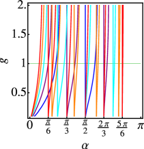
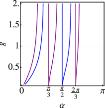
Figure 1: Asymptotic phase space of the mirror TBA (Left) and hybrid NLIE (Right) in the horizontal part. We set $s=3$ and $\gamma=0$ in hybrid NLIE. The lines correspond to $\alpha=\frac{n\pi}{Q}$ and the solutions of $T_{1,Q}(-\frac{i}{g})=0$ for $Q=2,3,4\dots$ (TBA) and $Q=2,3$ (NLIE). The phase space of the mirror TBA (Left) should be infinitesimally subdivided if $Q$ is not truncated at $Q=6$.

One remark is needed to evaluate the integrals in TBA and NLIE correctly in a numerical way. Consider the convolutions $\log(1+\mathfrak{a}_{s})\star K_{f}-\log(1+\overline{\mathfrak{a}}_{s})\star K_{f}^{[+2-2\gamma]}$ in $\left({\rm\ref{fa_s NLIE}}\right)$. If $(1+\mathfrak{a}_{s})$ crosses the branch cut of logarithm running the negative real axis, then the integrand changes discontinuously. Suppose there exists $v_{d}\in\mathbb{R}$ such that

$${\rm Im}\left[1+\mathfrak{a}_{s}(v_{d})\right]=0\ \ {\rm with}\ \ {\rm Re}\left[1+\mathfrak{a}_{s}(v_{d})\right]<0.$$ (2.20)

Then we need to integrate $\log(-1)=\pm\pi i$ over $(v_{d},\infty)$ or $(-\infty,v_{d})$, which provides extra source terms. As for asymptotic Konishi state, whenever $(1+\mathfrak{a}_{s})$ crosses the branch cut of logarithm, then $(1+\overline{\mathfrak{a}}_{s})$ crosses the branch cut at the same point. Thus we get

$$\Delta J_{s} =-\log\left[S_{f}(v-v_{d})S_{f}\Big{(}v-v_{d}+\frac{2i\,(1-\gamma)}{g}\Big{)}\right]-2\pi i,$$ (2.21)

$$\Delta\overline{J}_{s} =+\log\left[S_{f}(v-v_{d})S_{f}\Big{(}v-v_{d}-\frac{2i\,(1-\gamma)}{g}\Big{)}\right]+2\pi i.$$ (2.22)

The discontinuity of logarithm can in principle happen for the integral with $\log(1+Y_{s-2|w})$.

3 Contour deformation trick for TBA and NLIE

In the last section we studied the ground and orbifold Konishi states in the twisted AdS${}_{5}\times{}$S⁵, in which the hybrid NLIE acquires source terms. In this section, we turn our attention to the structure of the source term for general states. It is known that the origin of the source term in the simplified TBA for general states can be explained by both integration of Y-system and contour deformation trick. This is no longer trivially so in hybrid NLIE, as we shall see below.

3.1 General source terms in the simplified TBA

Take the simplified TBA for $Y_{1|w}$ as an example, and the following discussion applies to other simplified TBA equations as long as the Y-system exists at that node. We will derive the source terms by integration of Y-system and contour deformation trick.

The explanation by integration of Y-system goes as follows. Consider the logarithmic derivative of Y-system for $Y_{1|w}$

$$\,dl\hskip 0.85358pt\left[Y_{1|w}^{-}\,Y_{1|w}^{+}\right]=\,dl\hskip 0.85358pt\left[\left(1+Y_{2|w}\right)\left(\frac{1-\frac{1}{Y_{-}}}{1-\frac{1}{Y_{+}}}\right)\right],\qquad dlf(v)\equiv\frac{\partial}{\partial v}\log f(v).$$ (3.1)

Suppose $Y_{1|w}(v)$ has a set of single zeroes $r_{j}$ inside the strip ${\mathcal{A}}_{-1,1}$ . If we take the convolution of $\left({\rm\ref{dl Ysys 1w}}\right)$ with $s_{K}$ , the left hand side becomes

$$\int_{\mathbb{R}}dt\;\frac{\partial}{\partial t}\log\left[Y_{1|w}(t^{-})Y_{1|w}(t^{+})\right]s_{K}(v-t)=\,dl\hskip 0.85358ptY_{1|w}(v)+2\pi i\sum_{j}s_{K}\left(v-r_{j}-\frac{i}{g}\right).$$ (3.2)

Here all solutions of $Y_{1|w}(r_{j})=0,\ r_{j}\in{\mathcal{A}}_{-1,1}$ must be summed. If we integrate both sides with respect to $v$, we obtain the simplified TBA equation $\left({\rm\ref{TBA Y1w}}\right)$ with

$$V_{1|w}=c_{1|w}-\sum_{j}\log S\left(v-r_{j}-\frac{i}{g}\right),$$ (3.3)

where $c_{1|w}$ is an integration constant fixed by the behavior $v\to\pm\infty$, where all Y-functions approach the ground state value.

The explanation by contour deformation trick goes as follows. We start from the simplified TBA equation $\left({\rm\ref{TBA Y1w}}\right)$ for the ground state, $V_{1|w}=c_{1|w}$ . To obtain the TBA equation for excited states, we regard the contour of integration in the right hand side of $\left({\rm\ref{TBA Y1w}}\right)$ as running somewhere far below in the complex plane. When we pull the deformed contour back to the real axis, we obtain additional terms by picking up the residues as

$$\log Y_{1|w} =\log(1+Y_{2|w})\star_{C_{2|w}}s_{K}+\log\frac{1-\frac{1}{Y_{-}}}{1-\frac{1}{Y_{+}}}\,\hat{\star}\,_{C_{y}}s_{K}\,,$$

$$=-V_{1|w}+\log(1+Y_{2|w})\star s_{K}+\log\frac{1-\frac{1}{Y_{-}}}{1-\frac{1}{Y_{+}}}\,\hat{\star}\,s_{K}\,,$$ (3.4)

where $C_{2|w}\,,C_{y}$ are the deformed contour for respective convolutions.

Let $\{\rho_{n}\}$ be a set of roots $Y_{1|w}(\rho_{n})=0$, where $\rho_{n}\in{\mathcal{A}}_{n-1,n}$ for $n\geq 1$ and $\rho_{n}\in{\mathcal{A}}_{n,n+1}$ for $n\leq-1$. From the Y-system $\left({\rm\ref{dl Ysys 1w}}\right)$ it follows that

$$1+Y_{2|w}(\rho_{n}^{\pm})=0\quad{\rm or}\quad 1-\frac{1}{Y_{-}(\rho_{n}^{\pm})}=0\quad{\rm or}\quad 1-\frac{1}{Y_{+}(\rho_{n}^{\pm})}=\infty,\qquad n\in\mathbb{Z}_{\neq 0}\,.$$ (3.5)

When we straighten the deformed contours of $\left({\rm\ref{TBA Y1w}}\right)$ running through the lower half plane, the source term $V_{1|w}$ becomes

$$V_{1|w}=c_{1|w}+\log S\left(v-\rho_{1}^{-}\right)+\log S\left(v-\rho_{-1}^{-}\right).$$ (3.6)

where the contributions from $\rho_{-n}\ (n\geq 2)$ vanish owing to $S^{-}S^{+}=1$. This result agrees perfectly with $\left({\rm\ref{V1w TBA lemma}}\right)$.

3.2 General source terms in $A_{1}$ NLIE

3.2.1 Fourier transform method

The $A_{1}$ NLIE was derived from the assumptions that $Q^{[s-2]},L^{[+s]}$ are analytic in the upper half plane, and $\overline{Q}^{[2-s]},\overline{L}^{[-s]}$ are analytic in the lower half plane [18]. This derivation can be generalized to the case where dynamical variables have zeroes or poles in the complex plane:

$$T_{1,s}(t_{s,n})=T_{1,s}(t_{s,-n})=Q(q_{n})=\overline{Q}(\overline{q}_{n})=L(\ell_{n})=\overline{L}(\overline{\ell}_{n})=0,$$

$$\left\{t_{s,n}\,,\,q_{n}\,,\,\ell_{n}\right\}\in{\mathcal{A}}_{n-1,n}\,,\qquad\left\{t_{s,-n}\,,\,\overline{q}_{n}\,,\,\overline{\ell}_{n}\right\}\in{\mathcal{A}}_{-n,-n+1}\,,\qquad(n\geq 1).$$ (3.7)

In general, these functions can have multiple zeroes or poles in the complex plane. The generalization for such case is straightforward; if they have poles, the logarithmic derivative have the residue with the opposite sign. For simplicity we do not discuss poles.

The whole derivation is explained in Appendix D.1. Eventually we obtain the derivative of the source terms $J_{s}$ appearing in the hybrid NLIE $\left({\rm\ref{fa_s NLIE}}\right)$ as

$$J^{\prime}_{s}=J^{\prime}_{s}\Big{|}_{T}+J^{\prime}_{s}\Big{|}_{\overline{L}}+J^{\prime}_{s}\Big{|}_{L}+J^{\prime}_{s}\Big{|}_{\overline{Q}}+J^{\prime}_{s}\Big{|}_{Q}\,,$$ (3.8)

where

$$\frac{J^{\prime}_{s}}{2\pi i}\Big{|}_{T} =-K_{f}(v-t_{s,1}^{-})-K_{f}(v-t_{s,-1}^{-})-s_{K}(v-t_{s-1,1}^{-})-s_{K}(v-t_{s-1,-1}^{-}),$$ (3.9)

$$\frac{J^{\prime}_{s}}{2\pi i}\Big{|}_{\overline{L}} =-\sum_{n=1}^{\infty}\left\{K_{f}(v-\overline{\ell}_{s+n+1}^{[s-1]})+s_{K}(v-\overline{\ell}_{s+n}^{[s-2]})\right\},$$

$$\frac{J^{\prime}_{s}}{2\pi i}\Big{|}_{L} =-\sum_{n=1}^{\infty}\left\{K_{f}(v-\ell_{s+n+1}^{[-s-1]})+s_{K}(v-\ell_{s+n}^{[-s]})\right\}-\delta(v-\ell_{s+1}^{[-s-1]}),$$ (3.10)

$$\frac{J^{\prime}_{s}}{2\pi i}\Big{|}_{\overline{Q}} =\sum_{n=1}^{\infty}K_{1}(v-\overline{q}_{s+n-1}^{[s-2]}),$$

$$\frac{J^{\prime}_{s}}{2\pi i}\Big{|}_{Q} =\sum_{n=1}^{\infty}K_{1}(v-q_{s+n-1}^{[-s]})-\delta(v-q_{s+1}^{[-s-1]}).$$ (3.11)

We can neglect the $\delta$-functions, as they just add a constant after integration.

3.2.2 Contour deformation trick with Konishi’s contour

We start from the $A_{1}$ NLIE for the ground state with constant source terms $(J_{s}\,,\overline{J}_{s})=(j_{s}\,,\overline{\jmath}_{s})$. Then we apply the contour deformation trick to obtain extra source terms, using the same deformed contour as that of the orbifold Konishi state, depicted in Figure 2. For the NLIE of $\mathfrak{a}_{s}$ , it runs slightly above the line ${\rm Im}\,v=(1-s+\gamma)/g$, and run down along the imaginary axis. Note that the integrands have branch cut discontinuity along the line ${\rm Im}\,v=(1-s+\gamma)/g$. We take the limit $\gamma\ll 1$ in what follows.

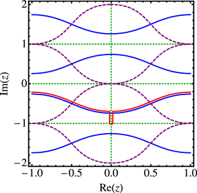
Figure 2: The deformed contour used in the NLIE for $\mathfrak{b}_{s}$ for the orbifold Konishi state. (Left) the contour in $z$-torus, where the vertical and horizontal axes are normalized by the period of the rapidity torus with moduli $k=-4g^{2}/Q^{2}$, with $Q=s-1$ for $(1+\mathfrak{b}_{s}),(1+\overline{\mathfrak{b}}_{s})$ and $Q=s-2$ for $(1+Y_{s-2|w})$. The real line in $z$-torus corresponds to the real axis of the mirror $v$-plane, and the line ${\rm Im}\,z=-1$ corresponds to the real axis of the string $v$-plane. We assumed that there are no singularities like Bethe roots along the string real axis. (Right) the contour in $v$-plane, where the orange region corresponds to the region surrounded by the deformed contour and the mirror real axis.

Again we throw the details of computation in Appendix D.2. After straightening the contour we obtain the following result:

$$J_{s}^{\rm CDT}=j_{s}-\log\left[S_{f}(v-t_{s,1}^{-})\,S_{f}(v-t_{s,-1}^{-})\right]-\log\left[S(v-t_{s-1,1}^{-})\,S(v-t_{s-1,-1}^{-})\right]\\[2.84526pt] -\log\left[\prod_{j=s+2}^{2s}S_{f}(v-\overline{\ell}_{j}^{[s-1]})\Big{/}\prod_{j=s+1}^{2s-2}S(v-\overline{\ell}_{j}^{[+s]})\right]+\log\left[\prod_{j=3}^{s+1}S_{f}(v-\ell_{j}^{[-s-1]})\cdot\prod_{j=3}^{s}S(v-\ell_{j}^{[-s]})\right]\\[2.84526pt] -\log\prod_{j=1}^{s-1}S_{1}(v-q_{j}^{[-s]})+\log\prod_{j=s}^{2s-2}S_{1}(v-\overline{q}_{j}^{[s-2]}).$$ (3.12)

3.2.3 Comparison

Let us compare the Fourier transform of the derivative of the source terms $\left({\rm\ref{FT J's}}\right)$ (Fourier source terms), with the source terms predicted by the contour deformation trick $\left({\rm\ref{CDT Js}}\right)$ (CDT source terms). We can make a similar argument for the NLIE of $\overline{\mathfrak{b}}_{s}$ . Since this is complex conjugate to $\mathfrak{b}_{s}$ , we just have to impose the complex-conjugate constraints in addition.

It turns out that there are mismatches in two results. Let us have a closer look for each of the T, L, Q-functions.

T-functions.

The Fourier source terms $\left({\rm\ref{Fourier T src}}\right)$ agree with the first line of the CDT source terms $\left({\rm\ref{CDT Js}}\right)$.

L-functions.

The Fourier source terms $\left({\rm\ref{Fourier LL src}}\right)$ partially agree with the second line of the CDT source terms $\left({\rm\ref{CDT Js}}\right)$.

The terms with $\{\overline{\ell}_{m}\}$ agree with each other if $\overline{\ell}_{m\geq 2s-1}$ lie along the imaginary axis in the lower half plane, so that all of them are picked up by the deformed contour.

The terms with $\{\ell_{m}\}$ do not agree, because they have the opposite signs. Moreover, the roots $\{\ell_{m}\}$ in $\left({\rm\ref{Fourier LL src}}\right)$ lie in the upper half plane, while those in $\left({\rm\ref{CDT Js}}\right)$ lie in the lower half plane.

Q-functions.

Just like the case of L-functions, The Fourier source terms $\left({\rm\ref{Fourier QQ src}}\right)$ partially agree with the third line of the CDT source terms $\left({\rm\ref{CDT Js}}\right)$.

If the deformed contour pick up all $\{\overline{q}_{m}\}$, then the terms with $\{\overline{q}_{m}\}$ perfectly agree with each other.

The terms with $\{q_{m}\}$ disagree. The roots $\{q_{s+n-1}^{[-s]}\}\ (n\geq 2)$ in $\left({\rm\ref{Fourier QQ src}}\right)$ lie in the upper half plane, while those in $\left({\rm\ref{CDT Js}}\right)$ lie in the lower half plane. The corresponding source terms have the opposite signs. One exception is $q_{s}^{[-s]}$ in the Fourier source term $\left({\rm\ref{Fourier QQ src}}\right)$. It lies in the lower half plane, but this term is not present in the CDT source term $\left({\rm\ref{CDT Js}}\right)$.

The mismatch between two source terms can be explained by different analyticity conditions used in two methods, as summarized in Table 1. In particular, the extra zeroes of $Q(v)$ at $v\in{\mathcal{A}}_{0,s-1}$ and those of $L(v)$ at $v\in{\mathcal{A}}_{2,s}$ modify only the CDT source terms.

Fourier	$Q^{[s-2]}\,,L^{[+s]}$ are meromorphic in the upper half plane.
CDT	$Q\,,L^{[+2]}$ are meromorphic in the upper half plane.

Table 1: Analyticity conditions used in the Fourier transformation method and the contour deformation trick. The complex conjugate conditions for $\overline{Q},\overline{L}$ are also used. We make no assumptions about $Q\,,L^{[+2]}$ in the lower half plane, $\overline{Q}\,,\overline{L}^{[-2]}$ in the upper half plane.

Strictly speaking, the T, L, Q-functions may have singularities which can be simultaneously removed by gauge transformation. We forbid such gauge artifacts, and assume that the roots $\{t_{s,n}\,,\ell_{n}\,,q_{n}\,,\overline{\ell}_{n}\,,\overline{q}_{n}\}$ are independent. In other words, the contour deformation trick with Konishi’s contour works fine as long as one can choose a gauge such that all zeroes and poles can be associated to the T-functions rather than the L- and Q-functions.

3.3 Consistent deformed contour

In the last subsection we have learned that, for states other than the orbifold Konishi, the contour deformation trick with Konishi’s contour may not yield the correct source terms of $A_{1}$ NLIE, as given by the Fourier transform method. To remedy this problem, we will look for new deformed contours of $A_{1}$ NLIE.

For the sake of simplicity let us choose the gauge $Q^{\rm I}=\overline{Q}^{\rm I}=1$. In other words, we will study the analyticity of gauge-invariant quantities,

$${\mathcal{T}}_{1,s}=\frac{T_{1,s}}{Q^{{\rm I}\,[+s]}\,\overline{Q}^{{\rm I}\,[-s]}}\,,\quad{\mathcal{L}}^{[+s]}=\frac{L^{[+s]}}{Q^{{\rm I}[+s]}\,Q^{{\rm I}\,[s-2]}}\,,\quad\overline{\mathcal{L}}^{[-s]}=\frac{\overline{L}^{[-s]}}{\overline{Q}^{{\rm I}[-s]}\,\overline{Q}^{{\rm I}\,[2-s]}}\,,$$ (3.13)

which enables us to rewrite

$$1+\mathfrak{b}_{s}^{\rm I}=\frac{{\mathcal{T}}_{1,s}^{+}}{{\mathcal{L}}^{[s+1]}}\,,\quad 1+\overline{\mathfrak{b}}_{s}^{\rm I}=\frac{{\mathcal{T}}_{1,s}^{-}}{\overline{\mathcal{L}}^{[-s-1]}}\,,\quad 1+Y_{1,s-1}=\frac{{\mathcal{T}}_{1,s-1}^{-}\,{\mathcal{T}}_{1,s-1}^{+}}{{\mathcal{L}}^{[+s]}\,\overline{\mathcal{L}}^{[-s]}}\,.$$ (3.14)

The zeroes of ${\mathcal{T}},{\mathcal{L}},\overline{\mathcal{L}}$ can be rephrased in terms of analyticity of $\mathfrak{b}_{s}\,,\overline{\mathfrak{b}}_{s}\,,Y_{1,s-1}$ as,

$${\mathcal{T}}_{1,s}=0\quad \leftrightarrow \quad 1+\mathfrak{b}_{s}^{-} =1+\overline{\mathfrak{b}}_{s}^{+} =0,$$

$${\mathcal{T}}_{1,s-1}=0\quad \leftrightarrow \quad 1+Y_{1,s-1}^{-} =1+Y_{1,s-1}^{+} =0,$$

$${\mathcal{L}}^{[+s]}=0\quad \leftrightarrow \quad 1+\mathfrak{b}_{s}^{-} =1+Y_{1,s-1} =\infty,$$

$$\overline{\mathcal{L}}^{[-s]}=0\quad \leftrightarrow \quad 1+\overline{\mathfrak{b}}_{s}^{+} =1+Y_{1,s-1} =\infty.$$ (3.15)

As in Section 3.2, we consider only the zeroes of ${\mathcal{T}},{\mathcal{L}},\overline{\mathcal{L}}$ and use the notation $\left({\rm\ref{def:zeroes TLQ}}\right)$. For completeness we also introduce ${\mathcal{L}}(\ell_{-n})=\overline{\mathcal{L}}(\overline{\ell}_{-n})=0$ with $\ell_{-n}\in{\mathcal{A}}_{-n,-n+1}\,,\overline{\ell}_{-n}\in{\mathcal{A}}_{n-1,n}$ for $n\geq 1$.

As a warm-up, let us apply the contour deformation trick to $A_{1}$ NLIE using the contour which encloses all zeroes of ${\mathcal{T}},{\mathcal{L}},\overline{\mathcal{L}}$ in the mirror sheet of complex $v$-plane. Just like the contour deformation trick in TBA, we do not pick up the singularities of the kernels. Let $*_{\downarrow}$ and $*_{\uparrow}$ be the deformed contours which encloses all zeroes in the lower and upper half plane when pulled backed to the real axis, and $*_{\updownarrow}\equiv*_{\downarrow}+*_{\uparrow}$. We then obtain

$$\log(1+\mathfrak{b}_{s})\star_{\updownarrow}K_{f}-\log(1+\overline{\mathfrak{b}}_{s})\star_{\updownarrow}K_{f}^{[+2]}+\log(1+Y_{1,s-1})\star_{\updownarrow}s_{K}\\ =-J_{s}^{\updownarrow}+\log(1+\mathfrak{b}_{s})\star K_{f}-\log(1+\overline{\mathfrak{b}}_{s})\star K_{f}^{[+2]}+\log(1+Y_{1,s-1})\star s_{K}\,,$$ (3.16)

with

$$-J_{s}^{\updownarrow}=+2\log\left[S_{f}(v-t_{s,1}^{-})S_{f}(v-t_{s,-1}^{-})S(v-t_{s-1,1}^{-})S(v-t_{s-1,-1}^{-})\right]\hskip 85.35826pt\\[2.84526pt] +\log\left[\prod_{n=1}^{\infty}S_{f}(v-\overline{\ell}_{s+1+n}^{[s-1]})S_{f}(v-\ell_{s+1+n}^{[-s-1]})S(v-\overline{\ell}_{s+n}^{[s-2]})S(v-\ell_{s+n}^{[-s]})\right]\\[2.84526pt] -\log\left[\prod_{k=-\infty,k\neq 0}^{s+1}S_{f}(v-\ell_{k}^{[-s-1]})\,S_{f}(v-\overline{\ell}_{k}^{[s-1]})\,\cdot\prod_{k=-\infty,k\neq 0}^{s}\frac{S(v-\ell_{k}^{[-s]})}{S(v-\overline{\ell}_{k}^{[+s]})}\right].$$ (3.17)

The derivation is discussed in Appendix D.2.2.

Let us compare the results with the Fourier source terms. The first line of $\left({\rm\ref{Js updown}}\right)$ involving the zeroes of T-functions is twice as large as $\left({\rm\ref{Fourier T src}}\right)$, and we should apply the principal value prescription to halve this contribution. The second line agrees with $\left({\rm\ref{Fourier LL src}}\right)$, which implies that the third line should be absent. It is easy to trace the origin of the third line. For example, $S(v-\ell_{k}^{[-s]})$ and $S_{f}(v-\ell_{k}^{[-s-1]})$ come from the zeroes of $L^{[+s]}$ and $L^{[+s+1]}$ in the lower half plane computed in $\left({\rm\ref{1+Ys down}}\right)$ and $\left({\rm\ref{BK down}}\right)$, respectively.

Based on this observation, we can specify a deformed contour which is consistent with the Fourier source terms. It turns out that, if we want to apply the contour deformation trick to the consistent deformed contour, we need to study the singularity of integrands first, and classify if they come from T-function or L-functions, following $\left({\rm\ref{classify TL zeroes}}\right)$.

Let us give one example of the consistent contour by modifying the contours $*_{\downarrow}\,,*_{\uparrow}$ to $*_{d}\,,*_{u}$ . For both $*_{d}$ and $*_{u}$ , we make the principal value prescription to the zeroes (or poles) of T-functions. As for $*_{d}$ , we neglect the zeroes of $L^{[+s]}$ or $L^{[s+1]}$ in the lower half plane, and as for $*_{u}$ we neglect the zeroes of $\overline{L}^{[-s]}$ or $\overline{L}^{[-s-1]}$ in the upper half plane. We join the two contours as shown in Figure 3, and denote the corresponding convolution by $*_{s}=*_{d}+*_{u}$ . We then obtain

$$\log(1+\mathfrak{b}_{s})\star_{s}K_{f}-\log(1+\overline{\mathfrak{b}}_{s})\star_{s}K_{f}^{[+2]}+\log(1+Y_{1,s-1})\star_{s}s_{K}\\ =-J_{s}^{\rm cons}+\log(1+\mathfrak{b}_{s})\star K_{f}-\log(1+\overline{\mathfrak{b}}_{s})\star K_{f}^{[+2]}+\log(1+Y_{1,s-1})\star s_{K}\,,$$ (3.18)

with

$$-J_{s}^{\rm cons}=\log\frac{S(v-t_{s-1,1}^{-})}{S(v-t_{s-1,-1}^{+})}+\log\left[\prod_{n=1}^{\infty}\frac{S(v-\ell_{s+n}^{[-s]})}{S(v-\overline{\ell}_{s+n}^{[+s]})}\right]\hskip 142.26378pt\\[2.84526pt] +\log\left[S_{f}(v-t_{s,1}^{-})S_{f}(v-t_{s,-1}^{-})\right]+\log\left[\prod_{n=1}^{\infty}S_{f}(v-\ell_{s+1+n}^{[-s-1]})S_{f}(v-\overline{\ell}_{s+1+n}^{[s-1]})\right].$$ (3.19)

The derivation is explained again in Appendix D.2.2. This result agrees with $\left({\rm\ref{Fourier T src}}\right)$, $\left({\rm\ref{Fourier LL src}}\right)$. Regarding the anti-holomorphic part of $A_{1}$ NLIE $\left({\rm\ref{fba_s NLIE}}\right)$, we can construct a consistent deformed contour by taking the complex conjugation.

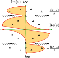
Figure 3: The deformed contour for $\mathfrak{b}_{s}\,,\overline{\mathfrak{b}}_{s}$ in $v$-plane, adjusted to be consistent with the Fourier source term. The symbols $\circ,\times,\triangle$ represent the zeroes or poles of $T,L,\overline{L}$, respectively. The orange region corresponds to the region surrounded by the deformed contour and the mirror real axis.

The source term $\left({\rm\ref{Js cons}}\right)$ depends on the zeroes (or poles) of $T_{1,s-1}\,,T_{1,s}$ in the strip ${\mathcal{A}}_{-1,1}$ and the zeroes (or poles) of $L,\overline{L}$ in the upper or lower half planes, $\{\ell_{s+1}\,,\ell_{s+2}\,,\dots\},\{\overline{\ell}_{s+1}\,,\overline{\ell}_{s+2}\,,\dots\}$. The latter is related to the poles (or zeroes) of dynamical variables $1+\mathfrak{b}_{s}^{-}\,,1+\overline{\mathfrak{b}}_{s}^{+}\,,1+Y_{1,s-1}$ via $\left({\rm\ref{classify TL zeroes}}\right)$. To impose the exact quantization condition on the extra roots lying outside the main strip, we need to analytically continue the NLIE, as mentioned in Section 2.3. This is a noticeable feature of NLIE compared to the mirror TBA.

4 Conclusion

In this paper we generalized the hybrid NLIE of [18] and applied it to a wider class of states.

First, we studied the ground and the orbifold Konishi states of twisted AdS${}_{5}\times{}$S⁵. In the mirror TBA, the orbifold Konishi states have infinitely many asymptotic critical lines from $Y_{M|w}$ nodes. In the hybrid NLIE, the number of critical lines is indeed reduced to a finite number. The quantization condition for the extra zeroes is written in terms of NLIE variables $(\mathfrak{a}_{s}\,,\overline{\mathfrak{a}}_{s}\,,Y_{1,s-1})$.

Second, we derived the source terms of hybrid NLIE for general states in two ways, Fourier transform method and contour deformation trick. We constructed the deformed contour which is consistent with the Fourier transform method.

It is interesting to generalize the gauge-invariant NLIE to $A_{n}$ cases. The $SU(N)$ principal chiral models contain boundstate spectrum for $N\geq 3$, and its NLIE has been studied in [72]. We should be able to reproduce their results by $A_{2}$ NLIE and contour deformation trick.

While this paper is in preparation, hybrid NLIE of AdS${}_{5}\times{}$S⁵ made out of $A_{1}$ and $A_{3}$ NLIE coupled to the quasi-local formulation of the mirror TBA [73] has appeared in [74]. We expect that the contour deformation trick will also work to obtain this new NLIE for excited states.

Acknowledgements

The author acknowledges Gleb Arutyunov and Stijn van Tongeren for discussions. This work is supported by the Netherlands Organization for Scientific Research (NWO) under the VICI grant 680-47-602.

Appendix A Notation

We follow the notation of [16, 18],

$$x_{s}(v)=\frac{v}{2}\left(1+\sqrt{1-\frac{4}{v^{2}}}\,\right),\qquad x(v)=\frac{1}{2}\left(v-i\sqrt{4-v^{2}}\,\right).$$

$${\mathcal{R}}_{(\pm)}(v)=\prod_{j=1}^{K}\frac{x(v)-x^{\pm}_{s,j}}{\sqrt{x^{\pm}_{s,j}}}\,,\quad{\mathcal{B}}_{(\pm)}(v)=\prod_{j=1}^{K}\frac{\frac{1}{x(v)}-x^{\pm}_{s,j}}{\sqrt{x^{\pm}_{s,j}}}\,,$$ (A.1)

together with $f^{[\pm m]}=f(v\pm\frac{im}{g})$ and $f(v)^{\pm}=f(v)^{[\pm 1]}$. The complex rapidity plane are divided into the strips,

$${\mathcal{A}}_{m,n}=\left\{v\in\mathbb{C}\ \Big{|}\ {\rm Im}\,v\in\left(\frac{m}{g}\,,\frac{n}{g}\right)\right\}.$$ (A.2)

We use the following kernels and S-matrices:

$$s_{K}(v) =\frac{1}{2\pi i}\,\frac{d}{dv}\log S(v) \quad S(v) =-\tanh[\frac{\pi}{4}(vg-i)]\,,$$

$$K_{Q}(v) =\frac{1}{2\pi i}\,\frac{d}{du}\,\log S_{Q}(v) \quad S_{Q}(v) =\frac{v-\frac{iQ}{g}}{u+\frac{iQ}{g}}\,,$$ (A.3)

$$K_{f}(v) =\frac{1}{2\pi i}\,\frac{\partial}{\partial v}\log S_{f}(v),\qquad \quad S_{f}(v) =\frac{\Gamma\left(\frac{g}{4\hskip 0.85358pti}\,(v+\frac{2i}{g})\right)\,\Gamma\left(-\frac{g\hskip 0.85358ptv}{4\hskip 0.85358pti}\right)}{\Gamma\left(\hskip 0.85358pt\frac{g\hskip 0.85358ptv}{4\hskip 0.85358pti}\right)\,\Gamma\left(-\frac{g}{4\hskip 0.85358pti}\,(v-\frac{2i}{g})\right)}\,.$$ (A.4)

One can check the properties $S^{+}S^{-}=1$ and $S_{f}^{-}S_{f}^{+}=S_{1}$ .

The convolutions are defined by

$$F\star K(v)=\int_{-\infty}^{\infty}dt\,F(t)\,K(v-t),\qquad F\,\hat{\star}\,K(v)=\int_{-2}^{2}dt\,F(t)\,K(v-t).$$ (A.5)

The logarithmic derivative and its Fourier transform are defined by

$$\,dl\hskip 0.85358ptX(v)\equiv\frac{\partial}{\partial v}\log X(v),\qquad\,\widehat{dl}\hskip 0.85358ptX(k)\equiv\int_{-\infty}^{+\infty}dv\;e^{ikv}\frac{\partial}{\partial v}\log X(v).$$ (A.6)

We also use $D_{k}=e^{k/g}$ and $\hat{s}_{K}=1/(D_{k}+D_{k}^{-1})$. It is useful to keep in mind that the operator $D_{k}$ shifts the location of zeroes,

$$D_{k}^{n}\,e^{ikq}=e^{ik\left(q-\frac{in}{g}\right)}=e^{ik\,q^{[-n]}},\qquad D_{k}^{-n}\,e^{ik\overline{q}}=e^{ik\,\overline{q}^{[+n]}}.$$ (A.7)

Another useful formulae are

$${\rm FT}^{-1}\left[\theta(+k)D_{k}^{+n}\frac{D_{k}-D_{k}^{-1}}{D_{k}+D_{k}^{-1}}\,e^{ikq}\right] =-K_{f}(v-q^{[-n]})-s_{k}(v-q^{[1-n]}),$$

$${\rm FT}^{-1}\left[\theta(-k)D_{k}^{-n}\frac{D_{k}-D_{k}^{-1}}{D_{k}+D_{k}^{-1}}\,e^{ikq}\right] =+K_{f}(v-q^{[+n]})+s_{k}(v-q^{[n-1]}).$$ (A.8)

The q-number is defined by

$$[s]_{q}=\frac{q^{s}-q^{-s}}{q-q^{-1}}\,,\qquad q=e^{i\alpha}\,.$$ (A.9)

Appendix B Review of NLIE variables

We briefly review the definition of dynamical variables $(\mathfrak{a}_{s}\,,\overline{\mathfrak{a}}_{s}\,,Y_{1,s-1})$ appearing in $A_{1}$ NLIE in terms of gauge-covariant variables, the T-, Q- and L-functions [18]. It is convenient to use the gauge-covariant variables when we explain how the source terms of $A_{1}$ NLIE appear or disappear in accordance with the analyticity of dynamical variables $(\mathfrak{a}_{s}\,,\overline{\mathfrak{a}}_{s}\,,Y_{1,s-1})$.

B.1 $A_{1}$ TQ-relations

It is known that the $A_{1}$ T-system can be linearized by the $A_{1}$ TQ-relations [75],

$$Q^{[s-2]}\,T_{1,s}-Q^{[+s]}\,T_{1,s-1}^{-}=\overline{Q}^{[-s]}\,L^{[+s]}\,,\quad\overline{Q}^{[2-s]}\,T_{1,s}-\overline{Q}^{[-s]}\,T_{1,s-1}^{+}=Q^{[+s]}\,\overline{L}^{[-s]}\,,$$ (B.1)

$$T_{0,s}\,T_{2,s}=L^{[+s+1]}\,\overline{L}^{[-s-1]}\,.$$

As a system of linear difference equations for $Q,\overline{Q}$, these equations have two linearly independent solutions. We distinguish them by $(Q,\overline{Q})$ and $(P,\overline{P})$ if necessary. We also notice that the equations $\left({\rm\ref{def:A1TQ}}\right)$ are covariant under the gauge transformation of T-system, as discussed in Appendix B.2. In particular, the gauge symmetry becomes manifest if we rewrite $\left({\rm\ref{def:A1TQ}}\right)$ using

$$(Q^{[+s]},P^{[+s]},\overline{Q}^{[-s]},\overline{P}^{[-s]},L^{[+s]},\overline{L}^{[-s]})=(Q_{1,s}^{\rm I},Q_{1,s}^{\rm II},\overline{Q}_{1,s}^{\rm I},\overline{Q}_{1,s}^{\rm II},L_{1,s},\overline{L}_{1,s}),$$ (B.2)

as

$$Q_{1,s-1}^{\nu\,-}\,T_{1,s}-Q_{1,s}^{\nu}\,T_{1,s-1}^{-}=\overline{Q}_{1,s-1}^{\nu\,-}\,L_{1,s}\,,\quad\overline{Q}_{1,s-1}^{\nu\,+}\,T_{1,s}-\overline{Q}_{1,s}^{\nu}\,T_{1,s-1}^{+}=Q_{1,s-1}^{\nu\,+}\,\overline{L}_{1,s}\,,$$ (B.3)

$$T_{0,s}\,T_{2,s}=L_{1,s}^{+}\,\overline{L}_{1,s}^{-}\,.$$

The $A_{1}$ NLIE is written by the gauge-invariant combination of variables in $\left({\rm\ref{covariant TQ}}\right)$ and of the T-system, namely

$$1+\mathfrak{b}_{s}^{\nu}=\frac{Q^{\nu\,[s-1]}}{\overline{Q}^{\nu\,[1-s]}}\,\frac{T_{1,s}^{+}}{L^{[s+1]}}\,,\quad 1+\overline{\mathfrak{b}}_{s}^{\nu}=\frac{\overline{Q}^{\nu\,[1-s]}}{Q^{\nu\,[s-1]}}\,\frac{T_{1,s}^{-}}{\overline{L}^{[-s-1]}}\,,\quad 1+Y_{1,s}=1+Y_{s-1|w}=\frac{T_{1,s}^{-}\,T_{1,s}^{+}}{T_{2,s}\,T_{0,s}}\,.$$ (B.4)

For regularization purposes, we define $\mathfrak{a}_{s}^{\nu}\,,\overline{\mathfrak{a}}_{s}^{\nu}$ and relate them to $\mathfrak{b}_{s}^{\nu}\,,\overline{\mathfrak{b}}_{s}^{\nu}$ as

$$\mathfrak{a}_{s}^{\nu}(v)=\mathfrak{b}_{s}^{\nu}\left(v-\frac{i\gamma}{g}\right),\qquad\overline{\mathfrak{a}}_{s}^{\nu}(v)=\overline{\mathfrak{b}}_{s}^{\nu}\left(v+\frac{i\gamma}{g}\right),\qquad(0<\gamma<1).$$ (B.5)

B.2 Symmetry in $A_{1}$ TQ-relations

The first line of $\left({\rm\ref{covariant TQ}}\right)$ is invariant under the holomorphic gauge transformation,

$$T_{1,s}\ \to\ g_{1}^{[+s]}\,g_{2}^{[-s]}\,T_{1,s}\,,\quad Q_{1,s}^{\nu}\ \to\ g_{1}^{[+s]}\,Q_{1,s}^{\nu}\,,\quad\overline{Q}_{1,s}^{\nu}\ \to\ g_{2}^{[-s]}\,\overline{Q}_{1,s}^{\nu}\,,$$ (B.6)

provided that the L-functions transform as

$$L_{1,s}^{+}\ \to\ g_{1}^{[s+1]}\,g_{1}^{[s-1]}\,L_{1,s}^{+}\,,\qquad\overline{L}_{1,s}^{-}\ \to\ g_{2}^{[-s+1]}\,g_{2}^{[-s-1]}\,\overline{L}_{1,s}^{-}\,.$$ (B.7)

The TQ-relations are also invariant under the anti-holomorphic transformation,

$$T_{1,s}\ \to\ g_{1}^{[+s]}\,g_{2}^{[-s]}\,T_{1,s}\,,\quad Q_{1,s}^{\nu}\ \to\ g_{2}^{[-s]}\,Q_{1,s}^{\nu}\,,\quad\overline{Q}_{1,s}^{\nu}\ \to\ g_{1}^{[+s]}\,\overline{Q}_{1,s}^{\nu}\,,$$ (B.8)

although it spoils the translational invariance of Q-functions $\left({\rm\ref{QPL translation}}\right)$. The combination of two transformations $\left({\rm\ref{trans holo}}\right)$, $\left({\rm\ref{trans anti-holo}}\right)$ generates a symmetry group larger than the usual gauge transformation of T-system.

The $Y$-functions and the variables $(\mathfrak{b}_{s}^{\nu}\,,\overline{\mathfrak{b}}_{s}^{\nu})$ are invariant under both transformations:

$$1+\mathfrak{b}_{s}^{\nu}=\frac{Q_{1,s-1}^{\nu}}{\overline{Q}_{1,s-1}^{\nu}}\,\frac{T_{1,s}^{+}}{L_{1,s}^{+}}\,,\qquad 1+\overline{\mathfrak{b}}_{s}^{\nu}=\frac{\overline{Q}_{1,s-1}^{\nu}}{Q_{1,s-1}^{\nu}}\,\frac{T_{1,s}^{-}}{L_{1,s}^{-}}\,.$$ (B.9)

However $(\mathfrak{b}_{s}^{\nu}\,,\overline{\mathfrak{b}}_{s}^{\nu})$ are not invariant under the frame rotation [68],

$$\begin{pmatrix}Q^{\prime}\\ P^{\prime}\end{pmatrix}=G\begin{pmatrix}Q\\ P\end{pmatrix},\qquad\begin{pmatrix}\overline{Q}^{\prime}\\ \overline{P}^{\prime}\end{pmatrix}=G\begin{pmatrix}\overline{Q}\\ \overline{P}\end{pmatrix},\qquad G^{+}=G^{-},\quad G\in SL(2,\mathbb{C}).$$ (B.10)

This transformation do not change Wronskians $T,L,\overline{L}$, but it acts on the index $\nu$ of $(\mathfrak{b}_{s}^{\nu}\,,\overline{\mathfrak{b}}_{s}^{\nu})$ in a non-linear way. As a result, the $A_{1}$ NLIEs before and after the transformation are related in a complicated way.

To write down NLIE we have to specify the frame, i.e. a particular direction of $\nu$. Due to the nonlinear transformation law of $(\mathfrak{b}_{s}^{\nu}\,,\overline{\mathfrak{b}}_{s}^{\nu})$ under the frame rotation, it seems to make little sense to consider the $A_{1}$ NLIE for general $\nu$, or general choice of frame.

B.3 General solution of $A_{1}$ TQ-relations

We look for the most general solution of $A_{1}$ TQ-relations for given Q-functions, and show that such solution is given by the Wronskian of Q-functions up to a periodic function.

Let us first introduce the differential form as [68, 76]

$$\mathbf{Q}(v)=\sum_{\nu={\rm I}}^{\rm II}Q^{\nu}(v)\,{\bf e}^{\nu},\qquad\overline{\mathbf{Q}}(v)=\sum_{\nu={\rm I}}^{\rm II}\overline{Q}^{\,\nu}(v)\,{\bf e}^{\nu},\qquad{\bf e}^{\rm I}\wedge{\bf e}^{\rm II}=1,$$ (B.11)

and rewrite the $A_{1}$ TQ-relations as

$$\mathbf{Q}^{[s-2]}\,T_{1,s}-\mathbf{Q}^{[+s]}\,T_{1,s-1}^{-}=\overline{\mathbf{Q}}^{[-s]}\,L_{1,s}\,,\quad\overline{\mathbf{Q}}^{[2-s]}\,T_{1,s}-\overline{\mathbf{Q}}^{[-s]}\,T_{1,s-1}^{+}=\mathbf{Q}^{[+s]}\,\overline{L}_{1,s}\,.$$ (B.12)

If we apply $\mathbf{Q}^{[+s]}\wedge$ and $\wedge\overline{\mathbf{Q}}^{[-s]}$ to both equations, we obtain

$$\mathbf{Q}^{[+s]}\wedge\mathbf{Q}^{[s-2]}\,T_{1,s} =\mathbf{Q}^{[+s]}\wedge\overline{\mathbf{Q}}^{[-s]}\,L_{1,s}\,, \quad\overline{\mathbf{Q}}^{[2-s]}\wedge\overline{\mathbf{Q}}^{[-s]}\,T_{1,s} =\mathbf{Q}^{[+s]}\wedge\overline{\mathbf{Q}}^{[-s]}\,\overline{L}_{1,s}\,,$$ (B.13)

$$\mathbf{Q}^{[s-2]}\wedge\overline{\mathbf{Q}}^{[-s]}\,T_{1,s} =\mathbf{Q}^{[+s]}\wedge\overline{\mathbf{Q}}^{[-s]}\,T_{1,s-1}^{-}\,, \quad\mathbf{Q}^{[+s]}\wedge\overline{\mathbf{Q}}^{[2-s]}\,T_{1,s} =\mathbf{Q}^{[+s]}\wedge\overline{\mathbf{Q}}^{[-s]}\,T_{1,s-1}^{+}\,.$$ (B.14)

The equations $\left({\rm\ref{A1TQ form2}}\right)$ are solved by the Ansatz

$$T_{1,s}=A_{1,s}\,\mathbf{Q}^{[+s]}\wedge\overline{\mathbf{Q}}^{[-s]},\qquad L_{1,s}=A_{1,s}\,\mathbf{Q}^{[+s]}\wedge\mathbf{Q}^{[s-2]},\qquad\overline{L}_{1,s}=A_{1,s}\,\overline{\mathbf{Q}}^{[2-s]}\wedge\overline{\mathbf{Q}}^{[-s]}\,,$$ (B.15)

and the equations $\left({\rm\ref{A1TQ form2}}\right)$ by

$$A_{1,s}=A_{1,s-1}^{-}=A_{1,s-1}^{+}\,.$$ (B.16)

Thus $A_{1,s}$ are periodic functions. This freedom should not be confused with gauge arbitrariness of $\left({\rm\ref{trans holo LL}}\right)$, because we have already chosen a particular gauge in writing $(\mathbf{Q}\,,\overline{\mathbf{Q}})$. These $A$’s cancel out in the combination $\left({\rm\ref{bbY from TLQ}}\right)$, so without loss of generality we may set them to unity. Then, the general solution $\left({\rm\ref{TLL general sol}}\right)$ becomes the Wronskian as

$$T_{1,s}=\mathbf{Q}^{[+s]}\wedge\overline{\mathbf{Q}}^{[-s]}={\rm det}\begin{pmatrix}Q^{[+s]}&\overline{Q}^{[-s]}\\ P^{[+s]}&\overline{P}^{[-s]}\\ \end{pmatrix},$$ (B.17)

$$L_{1,s}=\mathbf{Q}^{[+s]}\wedge\mathbf{Q}^{[s-2]}={\rm det}\begin{pmatrix}Q^{[+s]}&Q^{[s-2]}\\ P^{[+s]}&P^{[s-2]}\\ \end{pmatrix},\quad\overline{L}_{1,s}=\overline{\mathbf{Q}}^{[2-s]}\wedge\overline{\mathbf{Q}}^{[-s]}={\rm det}\begin{pmatrix}\overline{Q}^{[-s+2]}&\overline{Q}^{[-s]}\\ \overline{P}^{[-s+2]}&\overline{P}^{[-s]}\end{pmatrix}.$$

Appendix C Twisted asymptotic data

Below we summarize the data to solve the mirror TBA and hybrid NLIE for twisted AdS${}_{5}\times{}$S⁵ in the asymptotic limit. In particular, we need the twisted transfer matrices written in the form of Wronskian to solve the hybrid NLIE asymptotically. All T-, L-, Q-functions in this appendix are asymptotic expressions, though we use the same notation as in Appendix B.

C.1 Generalities

The twisted transfer matrices of $\mathfrak{su}(2|2)$ symmetry can be constructed by the generating functional called quantum characteristic function [70, 48]. In particular, the quantum characteristic function $D_{0}$ generates $T_{1,s}$ through

$$D_{0} =\left(1-U_{0}T_{1}U_{0}\right)\left(1-U_{0}T_{2}U_{0}\right)^{-1}\left(1-U_{0}T_{3}U_{0}\right)^{-1}\left(1-U_{0}T_{4}U_{0}\right),$$

$$\equiv\sum_{s=0}^{\infty}(-1)^{s}\,U_{0}^{s}\,T_{1,s}(x_{0}^{[\pm s]})\,U_{0}^{s}\,,$$ (C.1)

where $U_{0}$ is the shift operator acting on the mirror rapidity,

$$U^{s}\hskip 0.85358ptf(v)\hskip 0.85358ptU^{-s}\equiv f\Big{(}v+\frac{is}{g}\Big{)}=f^{[+s]}\,.$$ (C.2)

The $T_{n}$ are the components of the fundamental transfer matrix, $T_{1,1}=T_{1}-T_{2}-T_{3}+T_{4}$ , and they can be written as [77],

$$T_{n}=S_{0}\,\tilde{T}_{n}\,,\qquad S_{0}\equiv\prod_{j=1}^{K^{\rm II}}\frac{y_{j}-x^{-}_{0}}{y_{j}-x^{+}_{0}}\sqrt{\frac{x^{+}_{0}}{x^{-}_{0}}}\,\cdot\prod_{i=1}^{K^{\rm I}}\frac{x^{+}_{0}-x^{+}_{i}}{x_{0}^{+}-x_{i}^{-}}\sqrt{\frac{x_{i}^{-}}{x_{i}^{+}}}\,,$$ (C.3)

with

$$\tilde{T}_{1} =\prod_{j=1}^{K^{\rm II}}\frac{\nu_{j}-v-\frac{i}{g}}{\nu_{j}-v+\frac{i}{g}}\,\prod_{i=1}^{K^{\rm I}}\frac{1-\frac{1}{x_{0}^{-}x_{i}^{+}}}{1-\frac{1}{x_{0}^{-}x_{i}^{-}}}\sqrt{\frac{x_{i}^{+}}{x_{i}^{-}}}\,, \qquad\tilde{T}_{2} =e^{+i\alpha}\,\prod_{j=1}^{K^{\rm II}}\frac{\nu_{j}-v-\frac{i}{g}}{\nu_{j}-v+\frac{i}{g}}\,\prod_{k=1}^{K^{\rm III}}\frac{w_{k}-v+\frac{2i}{g}}{w_{k}-v}\,,$$

$$\tilde{T}_{3} =e^{-i\alpha}\prod_{k=1}^{K^{\rm III}}\frac{w_{k}-v-\frac{2i}{g}}{w_{k}-v}\,, \qquad\tilde{T}_{4} =\prod_{i=1}^{K^{\rm I}}\frac{x_{0}^{+}-x_{i}^{-}}{x^{+}_{0}-x^{+}_{i}}\sqrt{\frac{x_{i}^{+}}{x_{i}^{-}}}\,,$$ (C.4)

where we used $x_{0}=x(v),\,x_{i}=x_{s}(u_{i}),\,\nu_{j}=y_{j}+1/y_{j}$ , and introduced the twist by

$$T_{2}\to e^{i\alpha}\,T_{2}\,\qquad T_{3}\to e^{-i\alpha}\,T_{3}\,.$$ (C.5)

By expanding $\left({\rm\ref{def:D0}}\right)$, we obtain

$$T_{1,s} =\prod_{m=1}^{s}\left(-S_{0}^{[-s-1+2m]}\right)\cdot\left[\tilde{\rho}_{s+1}-\tilde{T}_{1}^{[-s+1]}\,\tilde{\rho}_{s}^{+}-\tilde{\rho}_{s}^{-}\,\tilde{T}_{4}^{[+s-1]}+\tilde{T}_{1}^{[-s+1]}\,\tilde{\rho}_{s-1}\,\tilde{T}_{4}^{[+s-1]}\right],$$ (C.6)

$$\tilde{\rho}_{s} =\prod_{m=1}^{s-1}\tilde{T}_{2}^{[-s+2m]}+\sum_{k=1}^{s-2}\left(\prod_{m=1}^{k}\tilde{T}_{2}^{[-s+2m]}\prod_{n=k+1}^{s-1}\tilde{T}_{3}^{[-s+2n]}\right)+\prod_{n=1}^{s-1}\tilde{T}_{3}^{[-s+2n]}\qquad(s\geq 2).$$ (C.7)

together with $\tilde{\rho}_{1}=1,\tilde{\rho}_{0}=0$. Note that

$$\prod_{m=1}^{s}\left(-S_{0}^{[-s-1+2m]}\right)=\prod_{j=1}^{K^{\rm II}}\frac{y_{j}-x^{[-s]}_{0}}{y_{j}-x^{[+s]}_{0}}\sqrt{\frac{x^{[+s]}_{0}}{x^{[-s]}_{0}}}\,\cdot\prod_{m=1}^{s}\left(-\frac{{\mathcal{R}}_{(+)}^{[-s+2m]}}{{\mathcal{R}}_{(-)}^{[-s+2m]}}\right).$$ (C.8)

The transfer matrices $T_{1,s}$ $\left({\rm\ref{T1s by rho}}\right)$ can be expressed as the Wronskian of Q-functions in the following way. Let us rewrite $\tilde{\rho}_{s\geq 1}$ as

$$\tilde{\rho}_{s}=\frac{U_{3}^{[s-1]}}{U_{2}^{[1-s]}}\sum_{k=0}^{s-1}\varrho^{[-s+1+2k]}\,,\qquad\varrho\equiv\frac{U_{2}}{U_{3}}\,,\quad\tilde{T}_{2}\equiv\frac{U_{2}^{+}}{U_{2}^{-}}\,,\quad\tilde{T}_{3}\equiv\frac{U_{3}^{+}}{U_{3}^{-}}\,,$$ (C.9)

and “differencize” the summation

$$M_{\rho}^{+}-M_{\rho}^{-}=\varrho\quad\Rightarrow\quad M_{\rho}^{[+s]}-M_{\rho}^{[-s]}=\sum_{k=0}^{s-1}\varrho^{[-s+1+2k]}\,,\quad\tilde{\rho}_{s}=\frac{U_{3}^{[s-1]}}{U_{2}^{[1-s]}}\left(M_{\rho}^{[s]}-M_{\rho}^{[-s]}\right).$$ (C.10)

After a little algebra, $\left({\rm\ref{T1s by rho}}\right)$ becomes

$$T_{1,s}=\prod_{m=1}^{s}\left(-S_{0}^{[-s-1+2m]}\right)\cdot\frac{U_{3}^{[s-2]}}{U_{2}^{[2-s]}}\,{\sf T}_{1,s}\,,\qquad{\sf T}_{1,s}=\ {\rm det}\begin{pmatrix}{\sf Q}^{[+s]}&\overline{\sf Q}^{[-s]}\\ {\sf P}^{[+s]}&\overline{\sf P}^{[-s]}\\ \end{pmatrix},$$ (C.11)

where

$${\sf Q}^{[+s]} =\tilde{T}_{4}^{[s-1]}-\tilde{T}_{3}^{[s-1]}=\left[\prod_{i=1}^{K^{\rm I}}\frac{x_{0}^{[+s]}-x_{i}^{-}}{x_{0}^{[+s]}-x^{+}_{i}}\sqrt{\frac{x_{i}^{+}}{x_{i}^{-}}}-e^{-i\alpha}\prod_{k=1}^{K^{\rm III}}\frac{w_{k}-v-\frac{i(s+1)}{g}}{w_{k}-v-\frac{i(s-1)}{g}}\right],$$

$$\overline{\sf Q}^{[-s]} =\tilde{T}_{1}^{[1-s]}-\tilde{T}_{2}^{[1-s]}=\prod_{j=1}^{K^{\rm II}}\frac{\nu_{j}-v+\frac{i(s-2)}{g}}{\nu_{j}-v+\frac{is}{g}}\left[\prod_{i=1}^{K^{\rm I}}\frac{1-\frac{1}{x_{0}^{[-s]}x_{i}^{+}}}{1-\frac{1}{x_{0}^{[-s]}x_{i}^{-}}}\sqrt{\frac{x_{i}^{+}}{x_{i}^{-}}}-e^{+i\alpha}\,\prod_{k=1}^{K^{\rm III}}\frac{w_{k}-v+\frac{i(s+1)}{g}}{w_{k}-v+\frac{i(s-1)}{g}}\right],$$

$${\sf P}^{[+s]} =+\varrho^{[+s]}\,\tilde{T}_{4}^{[s-1]}-{\sf Q}^{[+s]}\,M_{\rho}^{[+s+1]}\,,$$

$$\overline{\sf P}^{[-s]} =-\varrho^{[-s]}\,\tilde{T}_{1}^{[1-s]}-\overline{\sf Q}^{[-s]}\,M_{\rho}^{[-s-1]}\,.$$ (C.12)

It follows that

$${\sf L}^{[+s]} \equiv{\rm det}\begin{pmatrix}{\sf Q}^{[+s]}&{\sf Q}^{[s-2]}\\ {\sf P}^{[+s]}&{\sf P}^{[s-2]}\\ \end{pmatrix} =\frac{\varrho^{[+s]}\tilde{T}_{3}^{[s-1]}}{\tilde{T}_{2}^{[s-1]}}\left(\tilde{T}_{4}^{[s-3]}{\sf Q}^{[+s]}-\tilde{T}_{2}^{[s-1]}{\sf Q}^{[s-2]}\right),$$

$$\overline{\sf L}^{[-s]} \equiv{\rm det}\begin{pmatrix}\overline{\sf Q}^{[-s+2]}&\overline{\sf Q}^{[-s]}\\ \overline{\sf P}^{[-s+2]}&\overline{\sf P}^{[-s]}\end{pmatrix} =\frac{\varrho^{[-s]}\tilde{T}_{2}^{[1-s]}}{\tilde{T}_{3}^{[1-s]}}\left(\tilde{T}_{1}^{[3-s]}\overline{\sf Q}^{[-s]}-\tilde{T}_{3}^{[1-s]}\overline{\sf Q}^{[2-s]}\right).$$ (C.13)

A few remarks are in order. First, since our twist $\left({\rm\ref{T2T3 twist}}\right)$ affects $T_{1,s}$ only through $\rho_{s}$ , the results $\left({\rm\ref{general QP}}\right)$ should formally agree with [78] modulo gauge transformation. Second, if one wants to solve a couple of difference equations $\left({\rm\ref{rho_s as sum}}\right)$ explicitly for specific states, it is important to choose a good gauge for T-functions. Third, for the purpose of getting the asymptotic solution of the hybrid NLIE, we do not have to compute the second set of Q-functions $({\sf P},\overline{\sf P})$. Once we know ${\sf T}_{1,s}\,,{\sf Q},\overline{\sf Q}$, we obtain ${\sf L},\overline{\sf L}$ by the $A_{1}$ TQ-relations, and they provide sufficient data to construct the gauge-invariant variables $(\mathfrak{b}_{s}\,,\overline{\mathfrak{b}}_{s})$. Fourth, as will be discussed in $\left({\rm\ref{trans holo}}\right)$, there exists a gauge transformation of T-system which brings the first (or second) set of Q-functions to unity.

C.2 Transfer matrix for orbifold Konishi

Consider the orbifold Konishi state. Since ${K^{\rm II}}={K^{\rm III}}=0$, it satisfies

$$\tilde{\rho}_{s}=\sum_{k=1}^{s}e^{i\alpha(s+1-2k)}=\frac{e^{i\alpha s}-e^{-i\alpha s}}{e^{i\alpha}-e^{-i\alpha}}=[s]_{q}\,,$$ (C.14)

where $[s]_{q}$ is the q-number $\left({\rm\ref{def:q-number}}\right)$. The difference equations $\left({\rm\ref{rho_s as sum}}\right)$, $\left({\rm\ref{differencize rho}}\right)$ have the solution

$$U_{2}=\frac{1}{U_{3}}=e^{\alpha gv/2},\qquad M_{\rho}=\frac{e^{\alpha gv}-1}{2i\sin\alpha}\,,\qquad(\alpha\neq\pi\mathbb{Z}).$$ (C.15)

We added a constant to $M_{\rho}$ to keep the limit $\alpha\to 0$ non-singular. The asymptotic Q-functions for the orbifold Konishi state are given by

$${\sf Q}^{[+s]} =\frac{{\mathcal{R}}_{(-)}^{[+s]}}{{\mathcal{R}}_{(+)}^{[+s]}}-e^{-i\alpha} \qquad\overline{\sf Q}^{[-s]} =\frac{{\mathcal{B}}_{(+)}^{[-s]}}{{\mathcal{B}}_{(-)}^{[-s]}}-e^{+i\alpha}\,,$$

$${\sf P}^{[+s]} =e^{\alpha(gv+is)}\,\frac{{\mathcal{R}}_{(-)}^{[+s]}}{{\mathcal{R}}_{(+)}^{[+s]}}-{\sf Q}^{[+s]}\,M_{\rho}^{[+s+1]}\,, \qquad\overline{\sf P}^{[-s]} =-e^{\alpha(gv-is)}\,\frac{{\mathcal{B}}_{(+)}^{[-s]}}{{\mathcal{B}}_{(-)}^{[-s]}}-\overline{\sf Q}^{[-s]}\,M_{\rho}^{[-s-1]}\,,$$ (C.16)

and the corresponding ${\sf T}_{1,s}$ defined in $\left({\rm\ref{T1s Wronskian}}\right)$ is

$${\sf T}_{1,s}=e^{\alpha gv}\left([s+1]_{q}-[s]_{q}\,\frac{{\mathcal{R}}_{(-)}^{[+s]}}{{\mathcal{R}}_{(+)}^{[+s]}}-[s]_{q}\,\frac{{\mathcal{B}}_{(+)}^{[-s]}}{{\mathcal{B}}_{(-)}^{[-s]}}+[s-1]_{q}\,\frac{{\mathcal{R}}_{(-)}^{[+s]}}{{\mathcal{R}}_{(+)}^{[+s]}}\,\frac{{\mathcal{B}}_{(+)}^{[-s]}}{{\mathcal{B}}_{(-)}^{[-s]}}\right).$$ (C.17)

We define the L-functions as the solution of the $A_{1}$ TQ-relations $\left({\rm\ref{def:A1TQ}}\right)$, which yields

$${\sf L}^{[+s]} =e^{\alpha g\left(v+\frac{i(s-2)}{g}\right)}\left(1+\frac{{\mathcal{R}}_{(-)}^{[+s]}}{{\mathcal{R}}_{(+)}^{[+s]}}\frac{{\mathcal{R}}_{(-)}^{[s-2]}}{{\mathcal{R}}_{(+)}^{[s-2]}}-2\cos\alpha\,\frac{{\mathcal{R}}_{(-)}^{[s-2]}}{{\mathcal{R}}_{(+)}^{[s-2]}}\right),$$

$$\overline{\sf L}^{[-s]} =e^{\alpha g\left(v-\frac{i(s-2)}{g}\right)}\left(1+\frac{{\mathcal{B}}_{(+)}^{[-s]}}{{\mathcal{B}}_{(-)}^{[-s]}}\frac{{\mathcal{B}}_{(+)}^{[2-s]}}{{\mathcal{B}}_{(-)}^{[2-s]}}-2\cos\alpha\,\frac{{\mathcal{B}}_{(+)}^{[2-s]}}{{\mathcal{B}}_{(-)}^{[2-s]}}\right).$$ (C.18)

It also follows that

$$T_{0,s}\,T_{2,s}=T_{1,s}^{+}\,T_{1,s}^{-}-T_{1,s-1}\,T_{1,s+1}=L^{[+s+1]}\,\overline{L}^{[-s-1]}=L_{1,s}^{+}\,\overline{L}_{1,s}^{-}.$$ (C.19)

Here is a caution for numerical computation. The Wronskian formulae can be numerically unstable at large $|v|$ due to the cancellation of two vectors $(Q,P)\sim(\overline{Q},\overline{P})$. To avoid this problem we should use the analytic expression like $\left({\rm\ref{orbKon T1s}}\right)$ instead of the Wronskian form $\left({\rm\ref{T1s Wronskian}}\right)$. This remark also applies to the L-functions $\left({\rm\ref{Wronskian LL}}\right)$.

Appendix D Derivations

We derive our claims in Sections 3.2 and 3.3.

D.1 Derivation of $A_{1}$ NLIE with source terms

Below we generalize the derivation of $A_{1}$ NLIE [18] assuming that T, L, Q-functions have zeroes in the complex plane as $\left({\rm\ref{def:zeroes TLQ}}\right)$, which we repeat here:

$$T_{1,s}(t_{s,n})=T_{1,s}(t_{s,-n})=Q(q_{n})=\overline{Q}(\overline{q}_{n})=L(\ell_{n})=\overline{L}(\overline{\ell}_{n})=0,$$

$$\left\{t_{s,n}\,,\,q_{n}\,,\,\ell_{n}\right\}\in{\mathcal{A}}_{n-1,n}\,,\qquad\left\{t_{s,-n}\,,\,\overline{q}_{n}\,,\,\overline{\ell}_{n}\right\}\in{\mathcal{A}}_{-n,-n+1}\,,\qquad(n\geq 1).$$ (D.1)

The $A_{1}$ TQ-relations $\left({\rm\ref{covariant TQ}}\right)$ suggest to study the following two variables:

$$1+\mathfrak{b}_{s} =\frac{Q^{[s-1]}\,T_{1,s}^{+}}{\overline{Q}^{[1-s]}\,L^{[s+1]}}\,, \quad\mathfrak{b}_{s} =\frac{Q^{[s+1]}\,T_{1,s-1}}{\overline{Q}^{[1-s]}\,L^{[s+1]}}\,,$$

$$1+\overline{\mathfrak{b}}_{s} =\frac{\overline{Q}^{[1-s]}\,T_{1,s}^{-}}{Q^{[s-1]}\,\overline{L}^{[-s-1]}}\,, \quad\overline{\mathfrak{b}}_{s} =\frac{\overline{Q}^{[-s-1]}\,T_{1,s-1}}{Q^{[s-1]}\,\overline{L}^{[-s-1]}}\,.$$ (D.2)

Our goal is to deduce the equation of the form $\log\mathfrak{b}_{s}=\log(1+\mathfrak{b}_{s})\star K_{f}+\dots$ by taking Fourier transform of the logarithmic derivative of these equations. See Appendix A for notation.

As a warm-up, consider the T-system at $(1,s-1)$,

$$\,\widehat{dl}\hskip 0.85358pt\left[T_{1,s-1}^{+}T_{1,s-1}^{-}\right]=\,\widehat{dl}\hskip 0.85358pt\left[(1+Y_{1,s-1})\,L^{[+s]}\,\overline{L}^{[-s]}\right].$$ (D.3)

When $T_{1,s-1}(v)$ has zeroes inside the strip ${\mathcal{A}}_{-1,1}$ , we find the relations:

$$\,\widehat{dl}\hskip 0.85358ptT_{1,s-1}^{+} =\int_{\mathbb{R}+\frac{i}{g}}dv^{\prime}\,e^{ik(v^{\prime}-\frac{i}{g})}\,\partial_{v^{\prime}}\log T_{1,s-1}(v^{\prime})=D_{k}\left\{\,\widehat{dl}\hskip 0.85358ptT_{1,s-1}-2\pi i\,e^{ikt_{s-1,1}}\right\},\quad D_{k}\equiv e^{+k/g},$$

$$\,\widehat{dl}\hskip 0.85358ptT_{1,s-1}^{-} =\int_{\mathbb{R}-\frac{i}{g}}dv^{\prime}\,e^{ik(v^{\prime}+\frac{i}{g})}\,\partial_{v^{\prime}}\log T_{1,s-1}(v^{\prime})=D_{k}^{-1}\left\{\,\widehat{dl}\hskip 0.85358ptT_{1,s-1}+2\pi i\,e^{ikt_{s-1,-1}}\right\}.$$ (D.4)

The equation $\left({\rm\ref{Tsys 1,s-1}}\right)$ becomes

$$\,\widehat{dl}\hskip 0.85358ptT_{1,s-1}=\,\widehat{dl}\hskip 0.85358pt\left[(1+Y_{1,s-1})\,L^{[+s]}\,\overline{L}^{[-s]}\right]\hat{s}_{K}+2\pi i\,\left[D_{k}\,e^{ikt_{s-1,1}}-D_{k}^{-1}\,e^{ikt_{s-1,-1}}\right]\hat{s}_{K}\,.$$ (D.5)

where $\hat{s}_{K}\equiv 1/(D_{k}+D_{k}^{-1})$.

The relations $\left({\rm\ref{TBA lemma Ts-1}}\right)$ can be generalized to the Q- and L-functions (see Figure 4):

$$\,\widehat{dl}\hskip 0.85358ptQ^{[r+n]} =D_{k}^{n}\,\widehat{dl}\hskip 0.85358ptQ^{[r]} -2\pi i\,D_{k}^{r+n}\sum_{j=1}^{n}e^{ikq_{r+j}},$$

$$\,\widehat{dl}\hskip 0.85358ptQ^{[r-n]} =D_{k}^{-n}\,\widehat{dl}\hskip 0.85358ptQ^{[r]} +2\pi i\,D_{k}^{r-n}\sum_{j=1}^{n}e^{ikq_{r-n+j}},$$

$$\,\widehat{dl}\hskip 0.85358pt\overline{Q}^{[-r-n]} =D_{k}^{-n}\,\widehat{dl}\hskip 0.85358ptQ^{[-r]} +2\pi i\,D_{k}^{-r-n}\sum_{j=1}^{n}e^{ik\overline{q}_{r+j}},$$

$$\,\widehat{dl}\hskip 0.85358pt\overline{Q}^{[-r+n]} =D_{k}^{n}\,\widehat{dl}\hskip 0.85358ptQ^{[-r]} -2\pi i\,D_{k}^{-r+n}\sum_{j=1}^{n}e^{ik\overline{q}_{r-n+j}},$$ (D.6)

with $r,n\in\mathbb{Z}_{\geq 1}$ . By taking the limit $n\to\infty$, we find

$$\,\widehat{dl}\hskip 0.85358ptQ^{[+s]} =+2\pi i\,D_{k}^{s}\sum_{n=1}^{\infty}e^{ikq_{s+n}}\quad{\rm for}\ {\rm Re}\,k>0, \left({\rm if}\ \ \lim_{n\to\infty}\ D_{k}^{-n}\,\widehat{dl}\hskip 0.85358ptQ^{[r+n]}\to 0\right)$$

$$\,\widehat{dl}\hskip 0.85358pt\overline{Q}^{[-s]} =-2\pi i\,D_{k}^{-s}\sum_{n=1}^{\infty}e^{ik\overline{q}_{s+n}}\quad{\rm for}\ {\rm Re}\,k<0, \left({\rm if}\ \ \lim_{n\to\infty}\ D_{k}^{n}\,\widehat{dl}\hskip 0.85358pt\overline{Q}^{[-r-n]}\to 0\right).$$ (D.7)

Figure 4: Zeroes of $Q^{[+s]}(v)$ and $\overline{Q}^{[+s]}(v)$. Notice that when $Q(v)$ has a zero at $v=q_{s+1}\in{\mathcal{A}}_{s,s+1}$ as in $\left({\rm\ref{def:zeroes TLQ}}\right)$, the shifted function $Q^{[+s]}(v)$ has a zero at $v=q_{s+1}^{[-s]}\in{\mathcal{A}}_{0,1}$ .

Important lemma.

In order to derive the NLIE of gauge-invariant variables, it is important to look for a combination of $1+\mathfrak{b}_{s}\,,1+\overline{\mathfrak{b}}_{s}$ which do not depend on $T_{1,s}$ . The answer is

$$\mathfrak{X}_{s}\equiv\frac{1+\mathfrak{b}_{s}^{-}}{1+\overline{\mathfrak{b}}_{s}^{+}}=\frac{Q^{[s-2]}Q^{[+s]}\overline{L}^{[-s]}}{\overline{Q}^{[-s]}\overline{Q}^{[2-s]}L^{[+s]}}\,.$$ (D.8)

We then assume that

$$Q^{[s-2]}\ {\rm and}\ L^{[+s]}\ \text{are meromorphic in the upper half plane},$$

$$\overline{Q}^{[2-s]}\ {\rm and}\ \overline{L}^{[-s]}\ \text{are meromorphic in the lower half plane}.$$ (D.9)

These assumptions are realistic, because $Q(v),L(v+\frac{2i}{g})$ do not have branch cuts for ${\rm Im}\,v>0$ and $s\geq 3$ in our setup. By applying $\,\widehat{dl}\hskip 0.85358pt$ on both sides of $\left({\rm\ref{def:fXs}}\right)$, we obtain

$$\,\widehat{dl}\hskip 0.85358pt\mathfrak{X}_{s} =2\pi i\!\!\mathop{\rm Res}_{\raisebox{-2.84526pt}{\scriptsize\ \quad\rm UHP}}\,\widehat{dl}\hskip 0.85358pt\frac{Q^{[s-2]}Q^{[+s]}}{L^{[+s]}}+\,\widehat{dl}\hskip 0.85358pt\frac{\overline{L}^{[-s]}}{\overline{Q}^{[-s]}\overline{Q}^{[2-s]}}\,,\qquad({\rm Re}\,k>0),$$

$$\,\widehat{dl}\hskip 0.85358pt\mathfrak{X}_{s} =\,\widehat{dl}\hskip 0.85358pt\frac{Q^{[s-2]}Q^{[+s]}}{L^{[+s]}}+2\pi i\!\!\mathop{\rm Res}_{\raisebox{-2.84526pt}{\scriptsize\ \quad\rm LHP}}\,\widehat{dl}\hskip 0.85358pt\frac{\overline{L}^{[-s]}}{\overline{Q}^{[-s]}\overline{Q}^{[2-s]}}\,,\qquad({\rm Re}\,k<0).$$ (D.10)

where $\mathop{\rm Res}_{\,\rm UHP}$ and $\mathop{\rm Res}_{\,\rm LHP}$ collect the residues in the upper and lower half planes, respectively. By using $\left({\rm\ref{hdl fXs applied}}\right)$ and $\,\widehat{dl}\hskip 0.85358pt\!f=\theta(+k)\,\widehat{dl}\hskip 0.85358pt\!f+\theta(-k)\,\widehat{dl}\hskip 0.85358pt\!f$, we obtain

$$\,\widehat{dl}\hskip 0.85358pt\frac{Q^{[s-2]}Q^{[s]}}{L^{[+s]}} =+\theta(-k)\,\widehat{dl}\hskip 0.85358pt\mathfrak{X}_{s}+2\pi i\mathop{\rm Res}\,\widehat{dl}\hskip 0.85358pt\mathfrak{X}_{s}\,,$$

$$\,\widehat{dl}\hskip 0.85358pt\frac{\overline{Q}^{[2-s]}\overline{Q}^{[-s]}}{L^{[-s]}} =-\theta(+k)\,\widehat{dl}\hskip 0.85358pt\mathfrak{X}_{s}+2\pi i\mathop{\rm Res}\,\widehat{dl}\hskip 0.85358pt\mathfrak{X}_{s}\,,$$ (D.11)

$$\mathop{\rm Res}\,\widehat{dl}\hskip 0.85358pt\mathfrak{X}_{s} \equiv\theta(+k)\!\mathop{\rm Res}_{\raisebox{-2.84526pt}{\scriptsize\ \quad\rm UHP}}\,\widehat{dl}\hskip 0.85358pt\frac{Q^{[s-2]}Q^{[+s]}}{L^{[+s]}}+\theta(-k)\!\mathop{\rm Res}_{\raisebox{-2.84526pt}{\scriptsize\ \quad\rm LHP}}\,\widehat{dl}\hskip 0.85358pt\frac{\overline{Q}^{[-s]}\overline{Q}^{[2-s]}}{\overline{L}^{[-s]}}\,,$$ (D.12)

The last term can be computed explicitly with the help of $\left({\rm\ref{hdlQ cor}}\right)$ as

$$\mathop{\rm Res}\,\widehat{dl}\hskip 0.85358pt\mathfrak{X}_{s}=\theta(+k)\left\{D_{k}^{s}\sum_{n=1}^{\infty}e^{ikq_{s+n}}+D_{k}^{s-2}\sum_{n=1}^{\infty}e^{ikq_{s-2+n}}-D_{k}^{s}\sum_{n=1}^{\infty}e^{ik\ell_{s+n}}\right\}\\[2.84526pt] +\theta(-k)\left\{-D_{k}^{-s}\sum_{n=1}^{\infty}e^{ik\overline{q}_{s+n}}-D_{k}^{-s+2}\sum_{n=1}^{\infty}e^{ik\overline{q}_{s-2+n}}+D_{k}^{-s}\sum_{n=1}^{\infty}e^{ik\overline{\ell}_{s+n}}\right\}.$$ (D.13)

NLIE for $\mathfrak{b}_{s}$.

In order to derive the $A_{1}$ NLIE with source terms, consider $\,\widehat{dl}\hskip 0.85358pt\mathfrak{b}_{s}$ in $\left({\rm\ref{def:bs su2}}\right)$,

$$\,\widehat{dl}\hskip 0.85358pt\mathfrak{b}_{s} =\,\widehat{dl}\hskip 0.85358ptQ^{[s+1]}+\,\widehat{dl}\hskip 0.85358ptT_{1,s-1}-\,\widehat{dl}\hskip 0.85358pt\overline{Q}^{[1-s]}-\,\widehat{dl}\hskip 0.85358ptL^{[s+1]}\,,$$

$$=D_{k}^{2}\left\{\,\widehat{dl}\hskip 0.85358ptQ^{[s-1]}-\,\widehat{dl}\hskip 0.85358ptL^{[s]}\,\hat{s}_{K}\right\}-\left\{\,\widehat{dl}\hskip 0.85358pt\overline{Q}^{[1-s]}-\,\widehat{dl}\hskip 0.85358pt\overline{L}^{[-s]}\hat{s}_{K}\right\}+\,\widehat{dl}\hskip 0.85358pt(1+Y_{1,s-1})\,\hat{s}_{K}$$

$$\qquad-2\pi i\,D_{k}^{s+1}\left[e^{ikq_{s+1}}+e^{ikq_{s}}-e^{ik\ell_{s+1}}\right]+2\pi i\left[D_{k}\,e^{ikt_{s-1,1}}-D_{k}^{-1}\,e^{ikt_{s-1,-1}}\right]\hat{s}_{K}\,.$$ (D.14)

To rewrite the quantities in the curly brackets, we use $\mathfrak{X}_{s}$ in $\left({\rm\ref{def:fXs}}\right)$. With the help of the formulae $\left({\rm\ref{hdl QQL}}\right)$ and

$$\,\widehat{dl}\hskip 0.85358pt\left[Q^{[s-2]}Q^{[+s]}\right] =\left(D_{k}+D_{k}^{-1}\right)\,\widehat{dl}\hskip 0.85358ptQ^{[s-1]}+2\pi i\left[D_{k}^{s-2}\,e^{ikq_{s-1}}-D_{k}^{s}\,e^{ikq_{s}}\right],$$

$$\,\widehat{dl}\hskip 0.85358pt\left[\overline{Q}^{[2-s]}\overline{Q}^{[-s]}\right] =\left(D_{k}+D_{k}^{-1}\right)\,\widehat{dl}\hskip 0.85358pt\overline{Q}^{[1-s]}-2\pi i\left[D_{k}^{2-s}\,e^{ik\overline{q}_{s-1}}-D_{k}^{-s}\,e^{ik\overline{q}_{s}}\right],$$ (D.15)

we obtain

$$\,\widehat{dl}\hskip 0.85358pt\mathfrak{b}_{s}=\left\{D_{k}^{2}\,\theta(-k)+\theta(k)\right\}\hat{s}_{K}\,\widehat{dl}\hskip 0.85358pt\mathfrak{X}_{s}+\,\widehat{dl}\hskip 0.85358pt(1+Y_{1,s-1})\,\hat{s}_{K}+2\pi i\,(D_{k}^{2}-1)\,\hat{s}_{K}\mathop{\rm Res}\,\widehat{dl}\hskip 0.85358pt\mathfrak{X}_{s}\\[2.84526pt] +2\pi i\left[-D_{k}^{s}\,e^{ikq_{s-1}}-D_{k}^{s}\,e^{ikq_{s}}-D_{k}^{2-s}\,e^{ik\overline{q}_{s-1}}+D_{k}^{-s}\,e^{ik\overline{q}_{s}}\right]\hat{s}_{K}\\[2.84526pt] -2\pi i\,D_{k}^{s+1}\left[e^{ikq_{s+1}}-e^{ik\ell_{s+1}}\right]+2\pi i\left[D_{k}\,e^{ikt_{s-1,1}}-D_{k}^{-1}\,e^{ikt_{s-1,-1}}\right]\hat{s}_{K}\,.$$ (D.16)

Since we want an equation of the form $\,\widehat{dl}\hskip 0.85358pt\mathfrak{b}_{s}=\,\widehat{dl}\hskip 0.85358pt(1+\mathfrak{b}_{s})\hat{K}_{f}+\dots$, we rewrite $\,\widehat{dl}\hskip 0.85358pt\mathfrak{X}_{s}$ as

$$\,\widehat{dl}\hskip 0.85358pt\mathfrak{X}_{s} =D_{k}^{-1}\,\widehat{dl}\hskip 0.85358pt(1+\mathfrak{b}_{s})-D_{k}\,\widehat{dl}\hskip 0.85358pt(1+\overline{\mathfrak{b}}_{s})+2\pi i\mathop{\rm Res}\,\widehat{dl}\hskip 0.85358pt\frac{1+\mathfrak{b}_{s}^{-}}{1+\overline{\mathfrak{b}}_{s}^{+}}\,,$$ (D.17)

$$\mathop{\rm Res}\,\widehat{dl}\hskip 0.85358pt\frac{1+\mathfrak{b}_{s}^{-}}{1+\overline{\mathfrak{b}}_{s}^{+}} =e^{ikt_{s,1}}+e^{ikq_{s-1}^{[-s+2]}}-e^{ik\overline{q}_{s}^{[+s]}}-e^{ik\ell_{s+1}^{[-s]}}+e^{ikt_{s,-1}}+e^{ik\overline{q}_{s-1}^{[s-2]}}-e^{ikq_{s}^{[-s]}}-e^{ik\overline{\ell}_{s+1}^{[+s]}},$$

The last line is the collection of the residues of $\,\widehat{dl}\hskip 0.85358pt(1+\mathfrak{b}_{s})$ inside ${\mathcal{A}}_{-1,0}$ and $\,\widehat{dl}\hskip 0.85358pt(1+\overline{\mathfrak{b}}_{s})$ inside ${\mathcal{A}}_{0,1}$ with appropriate shift.

In summary, Fourier transform of the derivative of $A_{1}$ NLIE with the source term is

$$\,\widehat{dl}\hskip 0.85358pt\mathfrak{b}_{s}=-{\rm FT}\,(J^{\prime}_{s})+\,\widehat{dl}\hskip 0.85358pt(1+\mathfrak{b}_{s})\hat{K}_{f}-\,\widehat{dl}\hskip 0.85358pt(1+\overline{\mathfrak{b}}_{s})\hat{K}_{f}^{[+2]}+\,\widehat{dl}\hskip 0.85358pt(1+Y_{1,s-1})\,\hat{s}_{K}\,,$$ (D.18)

where $\hat{K}_{f}=\left\{D_{k}\,\theta(-k)+D_{k}^{-1}\theta(k)\right\}\hat{s}_{K}$ is the Fourier transform of the kernel $K_{f}$ , and

$$-\frac{{\rm FT}\,(J^{\prime}_{s})}{2\pi i}=D_{k}\,\hat{K}_{f}\mathop{\rm Res}\,\widehat{dl}\hskip 0.85358pt\frac{1+\mathfrak{b}_{s}^{-}}{1+\overline{\mathfrak{b}}_{s}^{+}}+(D_{k}^{2}-1)\,\hat{s}_{K}\mathop{\rm Res}\,\widehat{dl}\hskip 0.85358pt\mathfrak{X}_{s}\\[2.84526pt] +\left[-D_{k}^{s}\,e^{ikq_{s-1}}-D_{k}^{s}\,e^{ikq_{s}}-D_{k}^{2-s}\,e^{ik\overline{q}_{s-1}}+D_{k}^{-s}\,e^{ik\overline{q}_{s}}\right]\hat{s}_{K}\\[2.84526pt] -D_{k}^{s+1}\left[e^{ikq_{s+1}}-e^{ik\ell_{s+1}}\right]+\left[D_{k}\,e^{ikt_{s-1,1}}-D_{k}^{-1}\,e^{ikt_{s-1,-1}}\right]\hat{s}_{K}\,.$$ (D.19)

Here $\mathop{\rm Res}\,\widehat{dl}\hskip 0.85358pt\mathfrak{X}_{s}$ is given in $\left({\rm\ref{app:Res fXs}}\right)$, and it consists of infinitely many terms. To obtain $\left({\rm\ref{fa_s NLIE}}\right)$, we have to apply the inverse Fourier transform and integrate with respect to $v$. The inverse Fourier transform of $\left({\rm\ref{FT J's}}\right)$ is remarkably simple and given by $\left({\rm\ref{summary J's}}\right)$. The integration constants can be fixed by consideration of the limit $v\to\pm\infty$.

Case of orbifold Konishi state.

Let us check if the above results are consistent with the source terms of $A_{1}$ NLIE for orbifold Konishi state discussed in Section 2.3. As for the asymptotic orbifold Konishi state, $Q^{[s-2]},L^{[+s]}$ are analytic in the upper half plane and $\overline{Q}^{[2-s]},\overline{L}^{[-s]}$ are analytic in the lower half plane. We have to take care of the extra zeroes of T-functions only.

Since the $A_{1}$ NLIE is written in terms of $(\mathfrak{a}_{s}\,,\overline{\mathfrak{a}}_{s})=(\mathfrak{b}_{s}^{[-\gamma]},\overline{\mathfrak{b}}_{s}^{[+\gamma]})$ we have to modify slightly the derivation. In $\left({\rm\ref{hdl fbs comp1}}\right)$ we applied $\,\widehat{dl}\hskip 0.85358pt$ to the definition of $\mathfrak{b}_{s}$ . If we use $\mathfrak{a}_{s}=\mathfrak{b}_{s}^{[-\gamma]}$, we obtain

$$\,\widehat{dl}\hskip 0.85358pt\mathfrak{a}_{s}=\,\widehat{dl}\hskip 0.85358pt\mathfrak{b}_{s}^{[-\gamma]}=D_{k}^{-\gamma}\left[\,\widehat{dl}\hskip 0.85358pt\mathfrak{b}_{s}+2\pi i\,e^{ikt_{s-1,-\gamma}}\right]$$ (D.20)

Actually we may neglect the residue term. After the inverse Fourier transform, it becomes a $\delta$-function, whose integration is just a constant. There is another reason why we do not have to take care of the extra zeroes of $T_{1,s-1}$ : the rapidity of $Y_{s-1|w}$ in $\left({\rm\ref{fa_s NLIE}}\right)$, $\left({\rm\ref{fba_s NLIE}}\right)$ is not shifted at all.

An important modification occurs at the equation $\left({\rm\ref{hres 1+b12}}\right)$, which changes as

$$\,\widehat{dl}\hskip 0.85358pt\mathfrak{X}_{s}\equiv D_{k}^{-1+\gamma}\,\widehat{dl}\hskip 0.85358pt(1+\mathfrak{a}_{s})-D_{k}^{1-\gamma}\,\widehat{dl}\hskip 0.85358pt(1+\overline{\mathfrak{a}}_{s})+2\pi i\mathop{\rm Res}\,\widehat{dl}\hskip 0.85358pt\frac{1+\mathfrak{a}_{s}^{[-1+\gamma]}}{1+\overline{\mathfrak{a}}_{s}^{[+1-\gamma]}}\,,$$ (D.21)

Now the last term is the collection of the residues of $\,\widehat{dl}\hskip 0.85358pt(1+\mathfrak{a}_{s})$ inside ${\mathcal{A}}_{-1+\gamma,0}$ and $\,\widehat{dl}\hskip 0.85358pt(1+\overline{\mathfrak{a}}_{s})$ inside ${\mathcal{A}}_{0,1-\gamma}$ with appropriate shift. Since both $(1+\mathfrak{a}_{s}^{[-1+\gamma]})$ and $(1+\overline{\mathfrak{a}}_{s}^{[+1-\gamma]})$ are proportional to $T_{1,s}$ , this means that the extra zeroes of $T_{1,s}$ inside the strip ${\mathcal{A}}_{-1+\gamma,1-\gamma}$ contribute to the source term $\left({\rm\ref{FT J's}}\right)$. The rest of the derivation goes without any change.

One can see that this conclusion is consistent with the critical behavior observed in $\left({\rm\ref{bj quantize}}\right)$, $\left({\rm\ref{cj quantize}}\right)$.

D.2 Contour deformation for $A_{1}$ NLIE

We discuss how to obtain extra source terms in $A_{1}$ NLIE by applying the contour deformation trick to various deformed contours. When we straighten the deformed contour of the NLIE in the presence of extra zeroes $\left({\rm\ref{def:zeroes TLQ}}\right)$, we obtain extra terms by collecting the residues. To simplify the discussion we remove the regulator $\gamma$ by taking the limit $\gamma\ll 1$.

The holomorphic part of $A_{1}$ NLIE for the ground state ($J_{s}=j_{s}$) takes the form

$$\log\mathfrak{b}_{s}=-J_{s}+\log(1+\mathfrak{b}_{s})\star K_{f}-\log(1+\overline{\mathfrak{b}}_{s})\star K_{f}^{[+2-0]}+\log(1+Y_{s-2|w})\star s_{K}\,,$$ (D.22)

where the variables in the right hand side are defined by $\left({\rm\ref{bbY from TLQ}}\right)$.

D.2.1 Deformed contour of orbifold Konishi state

For general asymptotic states, $Q,L^{[+2]}$ have no branch cuts in the upper half plane, $\overline{Q},\overline{L}^{[-2]}$ have no branch cuts in the lower half plane, excluding the real axis. Thus, we can pull the integration contour of $(1+\mathfrak{b}_{s}),(1+\overline{\mathfrak{b}}_{s})$ up to ${\rm Im}\,v=\pm(s-1)/g$ and that of $(1+Y_{s-2|w})$ up to $\pm(s-2)/g$. Around the imaginary axis we can further deform them toward $\pm\infty$.

Let $*_{K}$ be the convolution using Konishi’s deformed contour depicted in Figure 2. This contour can pick up all zeroes of T, L, Q-functions inside the strip ${\mathcal{A}}_{-s+1,0}$ or ${\mathcal{A}}_{-s+2,0}$ . Recalling our notation $\left({\rm\ref{def:zeroes TLQ}}\right)$, we find

$$\log(1+\mathfrak{b}_{s})\star_{K}K_{f} \to+\log\left[\frac{\displaystyle S_{f}(v-t_{s,1}^{-})\prod_{j=1}^{s-2}S_{f}(v-t_{s,-j}^{-})\prod_{j=1}^{s-1}S_{f}(v-q_{j}^{[1-s]})}{\displaystyle\prod_{j=s}^{2s-2}S_{f}(v-\overline{q}_{j}^{[s-1]})\prod_{j=3}^{s+1}S_{f}(v-\ell_{j}^{[-s-1]})}\right],$$

$$-\log(1+\overline{\mathfrak{b}}_{s})\star_{K}K_{f}^{[+2]} \to-\log\left[\frac{\displaystyle\prod_{j=2}^{s}S_{f}(v-t_{s,-j}^{-})\prod_{j=s}^{2s-2}S_{f}(v-\overline{q}_{j}^{[s-3]})}{\displaystyle\prod_{j=1}^{s-1}S_{f}(v-q_{j}^{[-s-1]})\prod_{j=s+2}^{2s}S_{f}(v-\overline{\ell}_{j}^{[s-1]})}\right],$$

$$\log(1+Y_{1,s-1})\star_{K}s_{K} \to+\log\left[\frac{\displaystyle\prod_{j=2}^{s-1}S(v-t_{s-1,-j}^{+})\cdot S(v-t_{s-1,1}^{-})\prod_{j=1}^{s-3}S(v-t_{s-1,-j}^{-})}{\displaystyle\prod_{j=3}^{s}S(v-\ell_{j}^{[-s]})\prod_{j=s+1}^{2s-2}S(v-\overline{\ell}_{j}^{[+s]})}\right],$$ (D.23)

We assume that all roots $t_{s,-n}(n\geq 1)$ lie along the imaginary axis, as they do for the orbifold Konishi state at weak coupling. Since the deformed contour pick up the corresponding residues, we can replace the upper bound of the product of S-matrices with $t_{s,-n}\,,t_{s-1,-n}$ by $\infty$.

After straightening the contour and using $S^{+}S^{-}=1$ and $S_{f}^{-}S_{f}^{+}=S_{1}$ , the source term $J_{s}$ in $\left({\rm\ref{NLIE fb Js}}\right)$ becomes

$$J_{s}^{\rm CDT}=j_{s}-\log\left[S_{f}(v-t_{s,1}^{-})\,S_{f}(v-t_{s,-1}^{-})\right]-\log\left[S(v-t_{s-1,1}^{-})\,S(v-t_{s-1,-1}^{-})\right]\\[2.84526pt] -\log\left[\frac{\displaystyle\prod_{j=1}^{s-1}S_{1}(v-q_{j}^{[-s]})}{\displaystyle\prod_{j=s}^{2s-2}S_{1}(v-\overline{q}_{j}^{[s-2]})}\cdot\frac{\displaystyle\prod_{j=s+2}^{2s}S_{f}(v-\overline{\ell}_{j}^{[s-1]})}{\displaystyle\prod_{j=3}^{s+1}S_{f}(v-\ell_{j}^{[-s-1]})}\cdot\frac{1}{\displaystyle\prod_{j=3}^{s}S(v-\ell_{j}^{[-s]})\prod_{j=s+1}^{2s-2}S(v-\overline{\ell}_{j}^{[+s]})}\right].$$ (D.24)

D.2.2 Various deformed contours

Below we will derive the results of Section 3.3.

The convolutions $*_{\downarrow}\,,*_{\uparrow}$ are defined as the integration with the deformed contour which encloses all zeroes in the lower and upper half plane when pulled backed to the real axis. Using these deformed contours we obtain the source terms

$$\log(1+Y_{1,s-1})\star_{\downarrow}s_{K}$$

$$\quad\to+\log\left[\frac{S(v-t_{s-1,1}^{-})}{S(v-t_{s-1,-1}^{+})}\left(\prod_{j=1}^{\infty}\frac{S(v-t_{s-1,-j}^{-})\,S(v-t_{s-1,-j}^{+})}{S(v-\overline{\ell}_{s+j}^{[+s]})\,S(v-\ell_{-j}^{[-s]})}\right)\frac{1}{\prod_{k=1}^{s}S(v-\ell_{k}^{[-s]})}\right],$$ (D.25)

$$\log(1+Y_{1,s-1})\star_{\uparrow}s_{K}$$

$$\quad\to-\log\left[\frac{S(v-t_{s-1,-1}^{+})}{S(v-t_{s-1,1}^{-})}\left(\prod_{j=1}^{\infty}\frac{S(v-t_{s-1,j}^{+})S(v-t_{s-1,j}^{-})}{S(v-\ell_{s+j}^{[-s]})S(v-\overline{\ell}_{-j}^{[+s]})}\right)\frac{1}{\prod_{k=1}^{s}S(v-\overline{\ell}_{k}^{[+s]})}\right].$$ (D.26)

Similarly, we get

$$\log(1+\mathfrak{b}_{s})\star_{\downarrow}K_{f} \to+\log\left[S_{f}(v-t_{s,1}^{-})\left(\prod_{j=1}^{\infty}\frac{S_{f}(v-t_{s,-j}^{-})}{S_{f}(v-\ell_{-j}^{[-s-1]})}\right)\frac{1}{\prod_{k=1}^{s+1}S_{f}(v-\ell_{k}^{[-s-1]})}\right],$$ (D.27)

$$\log(1+\mathfrak{b}_{s})\star_{\uparrow}K_{f} \to-\log\left[\frac{1}{S_{f}(v-t_{s,1}^{-})}\left(\prod_{j=1}^{\infty}\frac{S_{f}(v-t_{s,j}^{-})}{S_{f}(v-\ell_{s+1+j}^{[-s-1]})}\right)\right],$$ (D.28)

$$-\log(1+\overline{\mathfrak{b}}_{s})\star_{\downarrow}K_{f}^{[+2]} \to-\log\left[\frac{1}{S_{f}(v-t_{s,-1}^{-})}\left(\prod_{j=1}^{\infty}\frac{S_{f}(v-t_{s,-j}^{-})}{S_{f}(v-\overline{\ell}_{s+1+j}^{[s-1]})}\right)\right],$$ (D.29)

$$-\log(1+\overline{\mathfrak{b}}_{s})\star_{\uparrow}K_{f}^{[+2]} \to+\log\left[S_{f}(v-t_{s,-1}^{-})\left(\prod_{j=1}^{\infty}\frac{S_{f}(v-t_{s,j}^{-})}{S_{f}(v-\overline{\ell}_{-j}^{[s-1]})}\right)\frac{1}{\prod_{k=1}^{s+1}S_{f}(v-\overline{\ell}_{k}^{[s-1]})}\right].$$ (D.30)

By adding all of them as $*_{\updownarrow}=*_{\downarrow}+*_{\uparrow}$ and simplifying the result using $S^{+}S^{-}=1$, we obtain

$$\log(1+\mathfrak{b}_{s})\star_{\updownarrow}K_{f}-\log(1+\overline{\mathfrak{b}}_{s})\star_{\updownarrow}K_{f}^{[+2]}+\log(1+Y_{1,s-1})\star_{\updownarrow}s_{K}\\[2.84526pt] \to+2\log\left[S_{f}(v-t_{s,1}^{-})S_{f}(v-t_{s,-1}^{-})S(v-t_{s-1,1}^{-})S(v-t_{s-1,-1}^{-})\right]\hskip 85.35826pt\\[2.84526pt] +\log\Biggl{[}\left(\prod_{j=1}^{\infty}S_{f}(v-\overline{\ell}_{s+1+j}^{[s-1]})S_{f}(v-\ell_{s+1+j}^{[-s-1]})S(v-\ell_{s+j}^{[-s]})S(v-\overline{\ell}_{s+j}^{[s-2]})\right)\ \times\\[2.84526pt] \frac{1}{\prod_{j=1}^{\infty}S_{f}(v-\ell_{-j}^{[-s-1]})S_{f}(v-\overline{\ell}_{-j}^{[s-1]})S(v-\overline{\ell}_{-j}^{[s-2]})S(v-\ell_{-j}^{[-s]})}\ \times\\[2.84526pt] \frac{1}{\prod_{k=1}^{s+1}S_{f}(v-\ell_{k}^{[-s-1]})\,S_{f}(v-\overline{\ell}_{k}^{[s-1]})}\,\frac{1}{\prod_{k=1}^{s}S(v-\overline{\ell}_{k}^{[s-2]})S(v-\ell_{k}^{[-s]})}\Biggr{]},$$ (D.31)

which is $\left({\rm\ref{Js updown}}\right)$.

Another set of contours, $*_{d}$ and $*_{u}$ , are defined as the slight modification of $*_{\downarrow}$ and $*_{\uparrow}$ . For $*_{d}\,,*_{u}$ the contribution from the zeroes of T-functions is halved. The zeroes of $L^{[+s]}$ or $L^{[s+1]}$ in the lower half plane are neglected in $*_{d}$ , and the zeroes of $\overline{L}^{[-s]}$ or $\overline{L}^{[-s-1]}$ in the upper half plane are neglected in $*_{u}$ . The contour deformation tricks for $\left({\rm\ref{1+Ys down}}\right)$-$\left({\rm\ref{BBK up}}\right)$ are now modified as

$$\log(1+Y_{1,s-1})\star_{d}s_{K} \to+\frac{1}{2}\log\frac{S(v-t_{s-1,1}^{-})}{S(v-t_{s-1,-1}^{+})}-\log\left[\prod_{j=1}^{\infty}S(v-\overline{\ell}_{s+j}^{[+s]})\right],$$ (D.32)

$$\log(1+Y_{1,s-1})\star_{u}s_{K} \to+\frac{1}{2}\log\frac{S(v-t_{s-1,1}^{-})}{S(v-t_{s-1,-1}^{+})}+\log\left[\prod_{j=1}^{\infty}S(v-\ell_{s+j}^{[-s]})\right].$$ (D.33)

$$\log(1+\mathfrak{b}_{s})\star_{d}K_{f} \to+\frac{1}{2}\log\left[S_{f}(v-t_{s,1}^{-})\prod_{j=1}^{\infty}S_{f}(v-t_{s,-j}^{-})\right],$$ (D.34)

$$\log(1+\mathfrak{b}_{s})\star_{u}K_{f} \to+\frac{1}{2}\log\frac{S_{f}(v-t_{s,1}^{-})}{\prod_{j=1}^{\infty}S_{f}(v-t_{s,j}^{-})}+\log\left[\prod_{j=1}^{\infty}S_{f}(v-\ell_{s+1+j}^{[-s-1]})\right],$$ (D.35)

$$-\log(1+\overline{\mathfrak{b}}_{s})\star_{d}K_{f}^{[+2]} \to+\frac{1}{2}\log\frac{S_{f}(v-t_{s,-1}^{-})}{\prod_{j=1}^{\infty}S_{f}(v-t_{s,-j}^{-})}+\log\left[\prod_{j=1}^{\infty}S_{f}(v-\overline{\ell}_{s+1+j}^{[s-1]})\right],$$ (D.36)

$$-\log(1+\overline{\mathfrak{b}}_{s})\star_{u}K_{f}^{[+2]} \to+\frac{1}{2}\log\left[S_{f}(v-t_{s,-1}^{-})\prod_{j=1}^{\infty}S_{f}(v-t_{s,j}^{-})\right],$$ (D.37)

By adding all of them and using $*_{s}=*_{d}+*_{u}$ , we obtain

$$\log(1+\mathfrak{b}_{s})\star_{s}K_{f}-\log(1+\overline{\mathfrak{b}}_{s})\star_{s}K_{f}^{[+2]}+\log(1+Y_{1,s-1})\star_{s}s_{K}\\[2.84526pt] \to+\log\frac{S(v-t_{s-1,1}^{-})}{S(v-t_{s-1,-1}^{+})}+\log\left[\prod_{j=1}^{\infty}\frac{S(v-\ell_{s+j}^{[-s]})}{S(v-\overline{\ell}_{s+j}^{[+s]})}\right]\hskip 142.26378pt\\[2.84526pt] +\log\left[S_{f}(v-t_{s,1}^{-})S_{f}(v-t_{s,-1}^{-})\right]+\log\left[\prod_{j=1}^{\infty}S_{f}(v-\ell_{s+1+j}^{[-s-1]})S_{f}(v-\overline{\ell}_{s+1+j}^{[s-1]})\right],$$ (D.38)

which is $\left({\rm\ref{Js cons}}\right)$.

References

- [1] J. M. Maldacena, “The Large limit of superconformal field theories and supergravity,” Adv. Theor. Math. Phys. 2 (1998) 231 [Int. J. Theor. Phys. 38 (1999) 1113] [hep-th/9711200].
- [2] D. Bombardelli, D. Fioravanti and R. Tateo, “Thermodynamic Bethe Ansatz for planar AdS/CFT: A Proposal,” J. Phys. A A 42 (2009) 375401 [arXiv:0902.3930 [hep-th]].
- [3] N. Gromov, V. Kazakov, A. Kozak and P. Vieira, “Exact Spectrum of Anomalous Dimensions of Planar Supersymmetric Yang-Mills Theory: TBA and excited states,” Lett. Math. Phys. 91 (2010) 265 [arXiv:0902.4458 [hep-th]].
- [4] G. Arutyunov and S. Frolov, “Thermodynamic Bethe Ansatz for the x Mirror Model,” JHEP 0905 (2009) 068 [arXiv:0903.0141 [hep-th]].
- [5] G. Arutyunov and S. Frolov, “On String S-matrix, Bound States and TBA,” JHEP 0712 (2007) 024 [arXiv:0710.1568 [hep-th]].
- [6] G. Arutyunov and S. Frolov, “String hypothesis for the mirror,” JHEP 0903 (2009) 152 [arXiv:0901.1417 [hep-th]].
- [7] N. Gromov, V. Kazakov and P. Vieira, “Exact Spectrum of Anomalous Dimensions of Planar Supersymmetric Yang-Mills Theory,” Phys. Rev. Lett. 103 (2009) 131601 [arXiv:0901.3753 [hep-th]].
- [8] A. Cavaglia, D. Fioravanti and R. Tateo, “Extended Y-system for the correspondence,” Nucl. Phys. B 843 (2011) 302 [arXiv:1005.3016 [hep-th]].
- [9] J. Balog and A. Hegedus, “ mirror TBA equations from Y-system and discontinuity relations,” JHEP 1108 (2011) 095 [arXiv:1104.4054 [hep-th]].
- [10] J. Ambjorn, R. A. Janik and C. Kristjansen, “Wrapping interactions and a new source of corrections to the spin-chain/string duality,” Nucl. Phys. B 736 (2006) 288 [hep-th/0510171].
- [11] Z. Bajnok and R. A. Janik, “Four-loop perturbative Konishi from strings and finite size effects for multiparticle states,” Nucl. Phys. B 807 (2009) 625 [arXiv:0807.0399 [hep-th]].
- [12] N. Gromov, V. Kazakov and P. Vieira, “Exact Spectrum of Planar N=4 Supersymmetric Yang-Mills Theory: Konishi Dimension at Any Coupling,” Phys. Rev. Lett. 104 (2010) 211601 [arXiv:0906.4240 [hep-th]].
- [13] S. Frolov, “Konishi operator at intermediate coupling,” J. Phys. A A 44 (2011) 065401 [arXiv:1006.5032 [hep-th]].
- [14] F. Levkovich-Maslyuk, “Numerical results for the exact spectrum of planar ,” JHEP 1205 (2012) 142 [arXiv:1110.5869 [hep-th]].
- [15] S. Frolov, “Scaling dimensions from the mirror TBA,” arXiv:1201.2317 [hep-th].
- [16] G. Arutyunov, S. Frolov and R. Suzuki, “Exploring the mirror TBA,” JHEP 1005 (2010) 031 [arXiv:0911.2224 [hep-th]].
- [17] J. Suzuki, “Spinons in magnetic chains of arbitrary spins at finite temperatures,” J. Phys. A 32, (1999) 2341, [cond-mat/9807076].
- [18] R. Suzuki, “Hybrid Nlie for the Mirror ,” J. Phys. A A 44 (2011) 235401 [arXiv:1101.5165 [hep-th]].
- [19] A. Klümper, M. T. Batchelor, “An analytic treatment of finite-size corrections in the spin-1 antiferromagnetic XXZ chain,” J. Phys. A 23 (1990) L189.
- [20] A. Klümper, M. T. Batchelor and P. A. Pearce, “Central charges of the 6- and 19- vertex models with twisted boundary conditions,” J. Phys. A 24 (1991) 3111.
- [21] C. Destri and H. J. de Vega, “New approach to thermal Bethe ansatz,” hep-th/9203064.
- [22] C. Destri and H. J. de Vega, “New thermodynamic Bethe ansatz equations without strings,” Phys. Rev. Lett. 69 (1992) 2313.
- [23] C. Destri and H. J. De Vega, “Unified approach to thermodynamic Bethe Ansatz and finite size corrections for lattice models and field theories,” Nucl. Phys. B 438 (1995) 413 [hep-th/9407117].
- [24] R. Roiban, “On spin chains and field theories,” JHEP 0409 (2004) 023 [hep-th/0312218].
- [25] D. Berenstein and S. A. Cherkis, “Deformations of Sym and integrable spin chain models,” Nucl. Phys. B 702 (2004) 49 [hep-th/0405215].
- [26] K. Ideguchi, “Semiclassical strings on x /Z(M) and operators in orbifold field theories,” JHEP 0409 (2004) 008 [hep-th/0408014].
- [27] N. Beisert and R. Roiban, “Beauty and the twist: the Bethe ansatz for twisted Sym,” JHEP 0508 (2005) 039 [hep-th/0505187].
- [28] N. Beisert and R. Roiban, “The Bethe ansatz for Z(S) orbifolds of super Yang-Mills theory,” JHEP 0511 (2005) 037 [hep-th/0510209].
- [29] S. Ananth, S. Kovacs and H. Shimada, “Proof of all-order finiteness for planar beta-deformed Yang-Mills,” JHEP 0701 (2007) 046 [hep-th/0609149].
- [30] S. Ananth, S. Kovacs and H. Shimada, “Proof of ultra-violet finiteness for a planar non-supersymmetric Yang-Mills theory,” Nucl. Phys. B 783 (2007) 227 [hep-th/0702020 [HEP-TH]].
- [31] H. Lin, O. Lunin and J. M. Maldacena, “Bubbling AdS space and 1/2 BPS geometries,” JHEP 0410 (2004) 025 [hep-th/0409174].
- [32] O. Lunin and J. M. Maldacena, “Deforming field theories with U(1) x U(1) global symmetry and their gravity duals,” JHEP 0505 (2005) 033 [hep-th/0502086].
- [33] S. Frolov, “Lax pair for strings in Lunin-Maldacena background,” JHEP 0505 (2005) 069 [hep-th/0503201].
- [34] S. A. Frolov, R. Roiban and A. A. Tseytlin, “Gauge-string duality for superconformal deformations of super Yang-Mills theory,” JHEP 0507 (2005) 045 [hep-th/0503192].
- [35] S. A. Frolov, R. Roiban and A. A. Tseytlin, “Gauge-string duality for (non)supersymmetric deformations of super Yang-Mills theory,” Nucl. Phys. B 731 (2005) 1 [hep-th/0507021].
- [36] F. Fiamberti, A. Santambrogio, C. Sieg and D. Zanon, “Finite-size effects in the superconformal beta-deformed Sym,” JHEP 0808 (2008) 057 [arXiv:0806.2103 [hep-th]].
- [37] F. Fiamberti, A. Santambrogio, C. Sieg and D. Zanon, “Single impurity operators at critical wrapping order in the beta-deformed Sym,” JHEP 0908 (2009) 034 [arXiv:0811.4594 [hep-th]].
- [38] J. A. Minahan and C. Sieg, “Four-Loop Anomalous Dimensions in Leigh-Strassler Deformations,” arXiv:1112.4787 [hep-th].
- [39] D. V. Bykov and S. Frolov, “Giant magnons in TsT-transformed ,” JHEP 0807 (2008) 071 [arXiv:0805.1070 [hep-th]].
- [40] J. Gunnesson, “Wrapping in maximally supersymmetric and marginally deformed Yang-Mills,” JHEP 0904 (2009) 130 [arXiv:0902.1427 [hep-th]].
- [41] M. Beccaria and G. F. De Angelis, “On the wrapping correction to single magnon energy in twisted Sym,” Int. J. Mod. Phys. A 24 (2009) 5803 [arXiv:0903.0778 [hep-th]].
- [42] Z. Bajnok, A. Hegedus, R. A. Janik and T. Lukowski, “Five loop Konishi from AdS/CFT,” Nucl. Phys. B 827 (2010) 426 [arXiv:0906.4062 [hep-th]].
- [43] M. de Leeuw and T. Lukowski, “Twist operators in beta-deformed theory,” JHEP 1104 (2011) 084 [arXiv:1012.3725 [hep-th]].
- [44] M. Beccaria, F. Levkovich-Maslyuk and G. Macorini, “On wrapping corrections to GKP-like operators,” JHEP 1103 (2011) 001 [arXiv:1012.2054 [hep-th]].
- [45] C. Ahn, Z. Bajnok, D. Bombardelli and R. I. Nepomechie, “Finite-size effect for four-loop Konishi of the -deformed Sym,” Phys. Lett. B 693 (2010) 380 [arXiv:1006.2209 [hep-th]].
- [46] C. Ahn, Z. Bajnok, D. Bombardelli and R. I. Nepomechie, “TBA, Nlo Luscher correction, and double wrapping in twisted AdS/CFT,” JHEP 1112 (2011) 059 [arXiv:1108.4914 [hep-th]].
- [47] C. Ahn, D. Bombardelli and M. Kim, “Finite-size effects of -deformed at strong coupling,” Phys. Lett. B 710 (2012) 467 [arXiv:1201.2635 [hep-th]].
- [48] N. Gromov and F. Levkovich-Maslyuk, “Y-system and -deformed Super-Yang-Mills,” J. Phys. A A 44 (2011) 015402 [arXiv:1006.5438 [hep-th]].
- [49] G. Arutyunov, M. de Leeuw and S. J. van Tongeren, “Twisting the Mirror TBA,” JHEP 1102 (2011) 025 [arXiv:1009.4118 [hep-th]].
- [50] M. de Leeuw and S. J. van Tongeren, “Orbifolded Konishi from the Mirror TBA,” J. Phys. A A 44 (2011) 325404 [arXiv:1103.5853 [hep-th]].
- [51] M. de Leeuw and S. J. van Tongeren, “The spectral problem for strings on twisted ,” Nucl. Phys. B 860 (2012) 339 [arXiv:1201.1451 [hep-th]].
- [52] M. Beccaria and G. Macorini, “Y-system for Orbifolds of Sym,” JHEP 1106 (2011) 004 [Erratum-ibid. 1201 (2012) 112] [arXiv:1104.0883 [hep-th]].
- [53] K. Zoubos, “Review of AdS/CFT Integrability, Chapter IV.2: Deformations, Orbifolds and Open Boundaries,” Lett. Math. Phys. 99 (2012) 375 [arXiv:1012.3998 [hep-th]].
- [54] P. Dorey and R. Tateo, “Excited states by analytic continuation of TBA equations,” Nucl. Phys. B 482 (1996) 639 [hep-th/9607167].
- [55] P. Dorey and R. Tateo, “Excited states in some simple perturbed conformal field theories,” Nucl. Phys. B 515 (1998) 575 [hep-th/9706140].
- [56] G. Arutyunov, S. Frolov and S. J. van Tongeren, “Bound States in the Mirror TBA,” JHEP 1202 (2012) 014 [arXiv:1111.0564 [hep-th]].
- [57] D. Fioravanti, A. Mariottini, E. Quattrini and F. Ravanini, “Excited state Destri-De Vega equation for Sine-Gordon and restricted Sine-Gordon models,” Phys. Lett. B 390 (1997) 243 [hep-th/9608091].
- [58] A. Hegedus, “Finite size effects in the Ss model: Two component nonlinear integral equations,” Nucl. Phys. B 679 (2004) 545 [hep-th/0310051].
- [59] J. Suzuki, “Excited states nonlinear integral equations for an integrable anisotropic spin 1 chain,” J. Phys. A A 37 (2004) 11957 [hep-th/0410243].
- [60] A. Hegedus, “Nonlinear integral equations for finite volume excited state energies of the O(3) and O(4) nonlinear sigma-models,” J. Phys. A A 38 (2005) 5345 [hep-th/0412125].
- [61] A. Hegedus, “Nonlinear integral equations for the finite size effects of Rsos and vertex-models and related quantum field theories,” Nucl. Phys. B 732 (2005) 463 [hep-th/0507132].
- [62] A. Hegedus, F. Ravanini and J. Suzuki, “Exact finite size spectrum in super sine-Gordon model,” Nucl. Phys. B 763 (2007) 330 [hep-th/0610012].
- [63] A. Hegedus, “Finite size effects and 2-string deviations in the spin-1 Xxz chains,” J. Phys. A A 40 (2007) 12007 [arXiv:0706.1411 [hep-th]].
- [64] N. Gromov, V. Kazakov and P. Vieira, “Finite Volume Spectrum of 2D Field Theories from Hirota Dynamics,” JHEP 0912 (2009) 060 [arXiv:0812.5091 [hep-th]].
- [65] J. Caetano, “Unified approach to the Principal Chiral Field model at Finite Volume,” arXiv:1012.2600 [hep-th].
- [66] A. Klümper and P. A. Pearce, “Conformal weights of RSOS lattice models and their fusion hierarchies,” Physica A 183 (1992) 304.
- [67] A. Klümper, “Thermodynamics of the anisotropic spin-1/2 Heisenberg chain and related quantum chains,” Z. Phys. B 91 (1993) 507, [cond-mat/9306019].
- [68] N. Gromov, V. Kazakov, S. Leurent and D. Volin, “Solving the AdS/CFT Y-system,” arXiv:1110.0562 [hep-th].
- [69] C. Ahn, Z. Bajnok, D. Bombardelli and R. I. Nepomechie, “Twisted Bethe equations from a twisted S-matrix,” JHEP 1102 (2011) 027 [arXiv:1010.3229 [hep-th]].
- [70] N. Beisert, “The Analytic Bethe Ansatz for a Chain with Centrally Extended su(2—2) Symmetry,” J. Stat. Mech. 0701 (2007) P01017 [nlin/0610017 [nlin.SI]].
-
[71]
N. Gromov (presented by V. Kazakov), talk at “Conference on Integrability in Gauge and String Theory 2010,” in Nordita Stockholm, June, 2010.
http://agenda.albanova.se/contributionDisplay.py?contribId=258&confId=1561 - [72] V. Kazakov and S. Leurent, “Finite Size Spectrum of Principal Chiral Field from Discrete Hirota Dynamics,” arXiv:1007.1770 [hep-th].
- [73] J. Balog and A. Hegedus, “Quasi-local formulation of the mirror TBA,” JHEP 1205 (2012) 039 [arXiv:1106.2100 [hep-th]].
- [74] J. Balog and A. Hegedus, “Hybrid-NLIE for the AdS/CFT spectral problem,” arXiv:1202.3244 [hep-th].
- [75] I. Krichever, O. Lipan, P. Wiegmann and A. Zabrodin, “Quantum integrable systems and elliptic solutions of classical discrete nonlinear equations,” Commun. Math. Phys. 188 (1997) 267 [hep-th/9604080].
-
[76]
D. Volin, “Lecture notes on quantum integrability,” downloadable from
https://nordita.webex.com/mw0306ld/mywebex/personalroom/personalroom.do?siteurl=nordita&AT=meet&username=Nordita - [77] G. Arutyunov, M. de Leeuw, R. Suzuki and A. Torrielli, “Bound State Transfer Matrix for Superstring,” JHEP 0910 (2009) 025 [arXiv:0906.4783 [hep-th]].
- [78] N. Gromov, V. Kazakov, S. Leurent and Z. Tsuboi, “Wronskian Solution for AdS/CFT Y-system,” JHEP 1101 (2011) 155 [arXiv:1010.2720 [hep-th]].