Dual Features of Magnetic Susceptibility in Superconducting Cuprates: a comparison to inelastic neutron scattering

Abstract

Starting from the generalized $t-J-G$ model Hamiltonian, we analyze the spin response in the superconducting cuprates taking into account both local and itinerant spin components which are coupled to each other self-consistently. We demonstrate that derived expression reproduces the basic observations of neutron scattering data in $YBa_{2}Cu_{3}O_{6+y}$ compounds near the optimal doping level.

(Some figures in this article are in color only in the electronic version)

1 Introduction

Theoretical studies of layered cuprates can be broadly separated into two parts depending on whether the point of consideration is Mott insulator or a metal. Theories of Mott insulatorstheorymott departs from a Mott insulator/Heisen-berg antiferromagnet (AFM) at half-filling, and addresses the issue how superconductivity (SC) and metallicity arise upon doping. Another class of theories theoryFL explores the idea that the system’s behaviour is primarily governed by interactions at energies smaller than the fermionic bandwidth, while contributions from higher energies account only for the renormalizations of the input parameters. For the cuprates, the point of departure for such theories is a Fermi liquid (FL) at large doping, and the issue these theories address is how non-Fermi liquid physics and unconventional pairing arise upon reducing the doping. Correspondingly, two approaches are also used for the description of a dynamic spin susceptibility. In the itinerant case usually one employs the random phase approximation (RPA) dahm ; Onufrieva ; norman ; eremin05 ; chubukov ; schnyder and in a proximity to the antiferromagnetic state, the spin response above T_c is governed by the continuum of the antiferromagnetic spin fluctuations (paramagnons). In the superconducting $d_{x^{2}-y^{2}}$-wave state there is a feedback effect of superconductivity on the spin response which yields a formation of the spin resonance below T_c. While the behaviour of the spin response in the superconducting state of optimally and overdoped cuprate superconductors can be qualitatively and even quantitatively understood within this approach, the normal state data are not entirely captured by the RPA where the excitations are completely damped and structureless at high energies.

Within the localised type of approaches the situation is opposite. In this case one starts from the undoped situation of a two-dimensional antiferromagnet and studies how the spin excitations evolve upon introducing the finite amount of carriersshimahara ; ihle ; zavidonov ; sherman ; prelovsek ; yamase ; barabanov ; vladimirov . Here the spin response remains dual in nature as it assumes a mixture of the local spins described by the superexchange interaction $J$ and the itinerant carriers with tight-binding energy dispersion. This scenario seems to be more efficient in describing the normal state spin dynamics, but so far its application to the superconducting state was rather limited. So called downward dispersion of neutron scattering intensity is not reproduced in this approach.

Note, the hour-glass-shape dispersion observed in neutron scattering below T_c naturally calls for the explanation of the spin response in terms of dual character of the excitations. While the upward dispersion resembles the collective spin wave-like branch as in quasi-two dimensional antiferromagnet with short range spin fluctuation, the downward dispersion in the superconducting state can be nicely attributed to the feedback effects of the $d$-wave order parameter on the itinerant component. However, usually an interaction between both would introduce the repulsion between both branches and it is not ’a-priori’ clear how the total response would look in this case. In this paper we discuss the possible way how to describe both components (local and itinerant) on equal footing within one analytical scheme based on the Green’s function method.

2 Basic equation for quasiparticle operators.

The starting point for our analysis is the usual $t-J$ type Hamiltonian with additional density-density interaction term

$$H=\sum_{i,j,\sigma}{t_{ij}\varPsi_{i}^{pd,\sigma}\varPsi_{j}^{\sigma,pd}}+\frac{1}{2}\sum_{i,j}J_{ij}\left[S_{i}S_{j}-\frac{n_{i}n_{j}}{4}\right]+\frac{1}{2}\sum_{i,j}G_{ij}\delta_{i}\delta_{j}.$$ (1)

Here, $\varPsi_{i}^{pd,\sigma}(\varPsi_{j}^{\sigma,pd})$ are the creation (annihilation) operators for the composite quasiparticles within the conduction band of hole-doped cuprates written in terms of projective operators to obey the no-double occupancy constraint. The second and third terms describe the superexchange interaction between the spins and the screened Coulomb interaction of the doped carriers, respectively. $\delta$ is a number of holes per one unit cell. Note that the spin operator commutes with the density-density interaction and this it will not appear explicitly in the final expression for the spin susceptibility.

Let us begin with the equation of motion for Fourier-transform of the quasiparticle operator

$$i\hbar\frac{\partial\varPsi_{k}^{\uparrow,pd}}{\partial t}=\left[\varPsi_{k}^{\uparrow,pd},H\right].$$ (2)

The linearization of the commutator on the rhs of Eq. (2) can be performed via projection method on the space of creation and annihilation operators, in a similar way proposed previously roth ; beenen ; plakida . However, in contrast to the previous approachessherman ; vladimirov we keep also the molecular field terms, which are proportional to the Fourier-transform of the transverse spin and the density of holes. In particular, we approximate the commutator in (2) by:

$$i\hbar\frac{\partial\varPsi_{k}^{\uparrow,pd}}{\partial t}\cong\varepsilon_{k}\varPsi_{k}^{\uparrow,pd}+\Delta_{k}\varPsi_{-k}^{pd,\downarrow}+\frac{1}{N}\sum_{q}{t^{\prime}_{k-q}\varPsi_{k-q}^{\downarrow,pd}S_{q}^{+}}\\ +\frac{1}{2N}\sum_{q}{t^{\prime}_{k-q}\varPsi_{k-q}^{\uparrow,pd}\delta_{q}}-\frac{1}{2N}\sum_{q}{J_{q}\varPsi_{k-q}^{\downarrow,pd}S_{q}^{+}}\\ +\frac{1}{N}\sum_{q}{\left[G_{q}-\frac{J_{q}}{4}\right]\varPsi_{k-q}^{\downarrow,pd}\delta_{q}},$$ (3)

where $t^{\prime}_{k}=\sum_{j}t_{ij}(1-F_{j})\exp\left(ikR_{ij}\right)$, $J_{q}=2J_{1}(\cos q_{x}a+\cos q_{y}a)$ and $G_{q}=\sum_{j}G_{ij}\exp(iqR_{ij})$ are the Fourier-trans-forms of the hoping integrals, superexchange, and Coulomb interactions, respectively. In the following we also set the lattice constant $a$ to unity. $N$ is a number of Cu–sites in the copper–oxygen plane. Collecting terms which are proportional the hopping amplitude, $t_{jl}$, the following expression for the energy of quasiparticles is obtained

$$\varepsilon_{k}=\sum_{l}t_{jl}\left[\frac{1+\delta}{2}+\frac{2}{1+\delta}(1+2F_{l})\left\langle S_{j}^{z}S_{l}^{z}\right\rangle\right]e^{ikR_{jl}}.$$ (4)

The physical meaning of square brackets can be understood as follows. The antiferromagnetic spin correlations suppress effective hopping integral, while ferromagnetic ones increase it. Thus one should expect that $1+2F_{l}>0$. Note that overall the effective nearest neighbour hopping determined as $\left[\frac{1+\delta}{2}+\frac{2}{1+\delta}(1+2F_{1})\left\langle S_{0}^{z}S_{1}^{z}\right\rangle\right]$ is analogous to Gutzwiller’s projection $\frac{2\delta}{1+\delta}$ for the hopping integral anderson . We show below that the exact form of $F_{l}$ can be rigorously computed via carriers concentration $\delta$ and the spin-spin correlations functions, see Eq.(28).

Note, that the energy dispersion, Eq.(4), can be written in a conventional form of the tight-binding dispersion,

$$\varepsilon_{k}=2t_{eff}^{(1)}\left(\cos k_{x}a+\cos k_{y}a\right)+4t_{eff}^{(2)}\cos k_{x}a\cos k_{y}a.$$ (5)

but with effective hopping integrals

$$t_{eff}^{(1)}=t_{1}\left[P+\frac{1/2+F_{1}}{1+\delta}K_{1}\right],$$ (6)

$$t_{eff}^{(2)}=t_{2}\left[P+\frac{1/2+F_{2}}{1+\delta}K_{2}\right].$$ (7)

where for shortness we introduce $P=\frac{1+\delta}{2}$, and the spin-spin correlation functions $K_{n}=4\left\langle S_{0}^{z}S_{n}^{z}\right\rangle$ are calculated via the spin susceptibility expression in a self-consistent way for a given doping and temperature.

In the following section we will further proceed with the derivation of the dynamical spin susceptibility based on the basic equations of motion for the quasiparticle operators. This approach differs from the memory function method (MFF) sherman ; prelovsek ; vladimirov where a linearization of the equations for the Fourier-transform of the spin operators is not related to the basic equation for quasiparticale operator (3). In this regard our approach is closer to the conventional random phase approximation. However, it employs projecting operators which fulfil the anticommutator relation

$$\left\{\varPsi_{i}^{pd,\uparrow}\varPsi_{j}^{\uparrow,pd}\right\}=\left(\frac{1+\delta_{i}}{2}+S_{i}^{z}\right)\delta_{ij}.$$ (8)

which results in richer behavior of the spin susceptibility. Although this approach requires some intuitive knowledge on the behaviour of the physical system it has some advantages because (i) both static and dynamic susceptibilities can be calculated within one approximation scheme, based on (3), (ii) the extension of the formalism to the various symmetry-broken ground states such as superconducting or spin/charge density wave ordered states is straightforward by adding the corresponding terms in the linearized equation of motion, Eq.(3), and (iii) the correct asymptotic Fermi-liquid type behaviour of the susceptibilities, when spin-spin correlation functions become small and the system approaches the conventional Fermi-liquid regime is restored.

In particular, Eq.(3) contains the superconducting gap, $\Delta_{\bf k}$ which mean-field expression can be readily found

$$\Delta_{k}=\frac{1}{PN}\sum_{k^{\prime}}\biggr{[}J_{k-k^{\prime}}\left\langle\varPsi_{k^{\prime}}^{\uparrow,pd}\varPsi_{-k^{\prime}}^{\downarrow,pd}\right\rangle\\ -J_{k-k^{\prime}}\left\langle\varPsi_{k^{\prime}}^{\downarrow,pd}\varPsi_{-k^{\prime}}^{\uparrow,pd}\right\rangle-G^{\prime}_{k-k^{\prime}}\left\langle\varPsi_{k^{\prime}}^{\uparrow,pd}\varPsi_{-k^{\prime}}^{\downarrow,pd}\right\rangle\biggm{]}\\ +\frac{1}{PN}\sum_{k^{\prime}}\biggr{[}t_{k^{\prime}}\left\langle\varPsi_{k^{\prime}}^{\downarrow,pd}\varPsi_{-k^{\prime}}^{\uparrow,pd}\right\rangle-t_{k^{\prime}}^{F}\left\langle\varPsi_{k^{\prime}}^{\uparrow,pd}\varPsi_{-k^{\prime}}^{\downarrow,pd}\right\rangle\biggm{]}.$$ (9)

where $t_{k^{\prime}}=\sum_{j}{t_{ij}\exp(ikR_{ij})}$, $t_{k^{\prime}}^{F}=\sum_{j}{t_{ij}F_{j}\exp(ikR_{ij})}$ and $G^{\prime}_{q}=G_{q}-J_{q}/4$. One sees that both superexchange and density-density interactions are involved. The analysis of this equation for $J_{k-k^{\prime}}>G_{k-k^{\prime}}$, which we assume hereafter, reveals d${}_{x^{2}-y^{2}}-$wave symmetry to be the most stable solution with $\Delta_{k}=\Delta(T)(\cos k_{x}a-\cos k_{y}a)/2$.

3 Dynamic spin susceptibility.

A hierarchy of constructed equations of motion for determining the spin response contains five Green’s functions. The initial one in the absence of the long range order ($\langle S_{z}\rangle=0$) has the form

$$\omega\langle\langle S_{q}^{+}|S_{-q}^{-}\rangle\rangle=-\sum_{k^{\prime}}{(t_{k^{\prime}+q}-t_{k^{\prime}})\langle\langle\varPsi_{k^{\prime}}^{pd,\downarrow}\varPsi_{k^{\prime}+q}^{\uparrow,pd}|S_{-q}^{-}\rangle\rangle}+\\ +\sum_{i,l}{J_{i,l}e^{-iqR_{l}}\langle\langle S_{l}^{+}S_{i}^{z}-S_{l}^{z}S_{i}^{+}|S_{-q}^{-}\rangle\rangle},$$ (10)

where $t_{k}$ is the usual tight-binding Fourier-transform hopping integral on the square lattice including the nearest, next-nearest, and next-next-nearest neighbour hoppings (a bare dispersion). The second term

$$G_{loc}(\omega,q)=\sum{J_{i,l}e^{-iqR_{l}}\langle\langle S_{l}^{+}S_{i}^{z}-S_{l}^{z}S_{i}^{+}|S_{-q}^{-}\rangle\rangle}$$ (11)

refers to the contribution of the localized spins. Its form is determined by the same procedure as described in Refs. shimahara ; ihle ; zavidonov ; sherman ; barabanov

$$\omega G_{loc}(\omega,q)=-\frac{i}{\pi}J_{1}K_{1}(2-\gamma_{q})+\Omega_{q}^{2}\langle\langle S_{q}^{+}|S_{-q}^{-}\rangle\rangle$$ (12)

and $\Omega_{q}$ determines the frequency of collective local spin fluctuations (magnon-like)

$$\Omega_{q}^{2}=2J_{1}^{2}\alpha(2-\gamma_{q})(\Delta_{sp}-K_{1}(2+\gamma_{q})),$$ (13)

where $\Delta_{sp}$ is a dimensionless parameter of the so-called spin-gap, sherman ; prelovsek , $\gamma_{q}=\cos q_{x}a+\cos q_{y}a$, and $\alpha$ is a decoupling parameter, controlled by the sum rule $\langle S_{i}^{+}S_{i}^{-}\rangle=\frac{1}{2}(1-\delta)$, which is about $1.4$.

The first term on the right hand side of Eq. (10)

$$G_{it}(\omega,q)=\frac{1}{2}\sum_{k^{\prime}}{(t_{k^{\prime}+q}-t_{k^{\prime}})\langle\langle\varPsi_{k^{\prime}+q}^{\uparrow,pd}\varPsi_{k^{\prime}}^{pd,\downarrow}-\varPsi_{k^{\prime}}^{pd,\downarrow}\varPsi_{k^{\prime}+q}^{\uparrow,pd}|S_{-q}^{-}\rangle\rangle}$$

is determined by the dynamics of itinerant spins. To compute this function we use the following exact relationseremin1 ; eremin2

$$\sum_{k}{\varPsi_{k}^{pd,\downarrow}\varPsi_{k+q}^{\uparrow,pd}}=0,$$ (14)

$$\sum_{k}{\varPsi_{k+q}^{\uparrow,pd}\varPsi_{k}^{pd,\downarrow}}=S_{q}^{+}.$$ (15)

Using Eq. (3) we construct further equations for the Green’s functions

$$\langle\langle\varPsi_{k}^{pd,\downarrow}\varPsi_{k+q}^{\uparrow,pd}|S_{-q}^{-}\rangle\rangle=\frac{i}{2\pi}\chi_{k,q}+\frac{1}{N}\eta^{\prime}_{k,q}\langle\langle S_{q}^{+}|S_{-q}^{-}\rangle\rangle+\frac{\zeta_{k,q}}{N}D^{\prime}\left(\omega,q\right),$$ (16)

$$\langle\langle\varPsi_{k+q}^{\uparrow,pd}\varPsi_{k}^{pd,\downarrow}|S_{-q}^{-}\rangle\rangle=-\frac{i}{2\pi}\chi_{k,q}-\frac{1}{N}\eta^{\prime\prime}_{k,q}\langle\langle S_{q}^{+}|S_{-q}^{-}\rangle\rangle-\frac{\zeta_{k,q}}{N}D^{\prime\prime}\left(\omega,q\right).$$ (17)

Observe that here the new Green’s functions appear

$$D^{\prime}\left(\omega,q\right)=-\sum_{k^{\prime}}{(\varepsilon_{k^{\prime}+q}-\varepsilon_{k^{\prime}})\langle\langle\varPsi_{k^{\prime}}^{pd,\downarrow}\varPsi_{k^{\prime}+q}^{\uparrow,pd}|S_{-q}^{-}\rangle\rangle},$$ (18)

$$D^{{}^{\prime\prime}}\left(\omega,q\right)=\sum_{k^{\prime}}{(\varepsilon_{k^{\prime}+q}-\varepsilon_{k^{\prime}})\langle\langle\varPsi_{k^{\prime}+q}^{\uparrow,pd}\varPsi_{k^{\prime}}^{pd,\downarrow}|S_{-q}^{-}\rangle\rangle}.$$ (19)

Combining Eqs.(14)-(17) we find

$$D^{\prime}(\omega,q)=-\left\{\frac{iN}{2\pi}\chi(\omega,q)+\eta^{\prime}(\omega,q)\langle\langle S_{q}^{+}|S_{-q}^{-}\rangle\rangle\right\}/\zeta(\omega,q)$$ (20)

and

$$D^{\prime\prime}(\omega,q)=-\left\{\frac{iN}{2\pi}\chi(\omega,q)+\left[1+\eta^{{}^{\prime\prime}}(\omega,q)\right]\langle\langle S_{q}^{+}|S_{-q}^{-}\rangle\rangle\right\}/\zeta(\omega,q),$$ (21)

where for $T>T_{c}$

$$\chi(\omega,q)=\sum_{k}{\chi_{k,q}}=\frac{1}{N}\sum\frac{n_{k+q}-n_{k}}{\omega+\varepsilon_{k}-\varepsilon_{k+q}},$$ (22)

$$\zeta(\omega,q)=\sum_{k}{\zeta_{k,q}}=\frac{1}{N}\sum\frac{1}{\omega+\varepsilon_{k}-\varepsilon_{k+q}},$$ (23)

$$\eta^{\prime}(\omega,q)=\sum_{k}{\eta^{\prime}_{k,q}} = \frac{1}{2}J_{q}\chi(\omega,q)$$ (24)

$$- \frac{1}{N}\sum\frac{t^{\prime}_{k+q}n_{k+q}-t^{\prime}_{k}n_{k}}{\omega+\varepsilon_{k}-\varepsilon_{k+q}},$$

$$\eta^{{}^{\prime\prime}}(\omega,q)=\sum_{k}{\eta^{\prime\prime}_{k,q}} = \eta^{\prime}(\omega,q)$$ (25)

$$+ \frac{1}{N}\sum\frac{P(t^{\prime}_{k+q}-t^{\prime}_{k})-\omega}{\omega+\varepsilon_{k}-\varepsilon_{k+q}}.$$

We remind that the difference between $t_{k}$ and $t^{\prime}_{k}$ is expressed below Eq.(3) and $n_{k}=Pf_{k}$ where $f_{k}$ is a Fermi function. Taking into account that $\sum_{k^{\prime}}{(\varepsilon_{k^{\prime}+q}-\varepsilon_{k^{\prime}})=0}$ it is easy to prove that $D^{\prime}\left(\omega,q\right)=D^{{}^{\prime\prime}}\left(\omega,q\right)$. This means that Eqs.(20) and (21) are consistent with each other if the following relation holds

$$1+\frac{1}{N}\sum_{k}\frac{P(t^{\prime}_{k+q}-t^{\prime}_{k})-\omega}{\omega+\varepsilon_{k}-\varepsilon_{k+q}}=0.$$ (26)

This property can be used to express the projection parameter $F_{i}$ via the spin-spin correlation function $K_{i}$. For this we add and subtract $\varepsilon_{k}-\varepsilon_{k+q}$ in the numerator of Eq.(26) which yields the identity

$$\sum_{k}\frac{P(t^{\prime}_{k+q}-t^{\prime}_{k})-\varepsilon_{k+q}+\varepsilon_{k}}{\omega+\varepsilon_{k}-\varepsilon_{k+q}}=0.$$ (27)

Note that the remaining sum vanishes at any frequency if $P(t^{\prime}_{k+q}-t^{\prime}_{k})-\varepsilon_{k+q}+\varepsilon_{k}=0$. Equating factors in front of the independent trigonometric cosine functions results in the relation between $F_{i}$ and corresponding spin-spin correlation functions

$$F_{i}=\frac{-K_{i}}{(1+\delta)^{2}+2K_{i}}$$ (28)

which holds for any value of $i$. Recalling that $1+2F_{1}>0$, we find that $(1+\delta)^{2}>2|K_{1}|$. This condition implies that the concentration of carriers should be larger than some critical value $\delta_{0}$ to have the metallic behaviour of the system.

Having $D^{\prime}\left(\omega,q\right)$, $D^{\prime\prime}\left(\omega,q\right)$ and using Eqs.(16), (17) it is straightforward to find $G_{it}(\omega,q)$ and $\langle\langle S_{q}^{+}|S_{-q}^{-}\rangle\rangle$. The obtained system of coupled equations allow us to get a closed form for the Green’s function $\langle\langle S_{q}^{+}|S_{-q}^{-}\rangle\rangle$ i.e., for the spin susceptibility

$$\chi_{total}^{+,-}=\frac{\omega\chi(\omega,q)\zeta_{t}(\omega,q)-[\omega\chi_{t}(\omega,q)+2J_{1}K_{1}(2-\gamma_{q})]\zeta(\omega,q)}{\omega\left[1/2+\eta(\omega,q)\right]\zeta_{t}(\omega,q)+[\Omega_{q}^{2}-\omega^{2}-\omega\eta_{t}(\omega,q)]\zeta(\omega,q)}.$$ (29)

Here,

$$\eta(\omega,q)=\frac{1}{2}J_{q}\chi(\omega,q)\\ -\frac{1}{N}\sum_{k}{\frac{t_{k+q}^{\prime}(n_{k+q}-P/2)-t_{k}^{\prime}(n_{k}-P/2)}{\omega+\varepsilon_{k}-\varepsilon_{k+q}}},$$ (30)

and

$$\zeta_{t}(\omega,q) = \frac{P}{N}\sum_{k}(t_{k+q}-t_{k})\zeta_{k,q},$$

$$\chi_{t}(\omega,q) = \frac{P}{N}\sum_{k}(t_{k+q}-t_{k})\chi_{k,q},$$ (31)

$$\eta_{t}(\omega,q) = \frac{P}{N}\sum_{k}(t_{k+q}-t_{k})\eta_{k,q}.$$

Note that the analytic continuation $\omega=\omega+i0^{+}$ used in the derivation is replaced in the numerical calculations by $\omega=\omega+i\varGamma$ where $\varGamma$ is a small numerical factor. It is frequency independent and resembles the effect of the non-magnetic impurity scattering. norman ; eremin05 ; chubukov ; schnyder

Let us turn now to the situation of the superconducting state, $T<T_{c}$. Performing the Bogolyubov transformations for the quasiparticle states and obtaining the new Eigenenergies $E_{k}$, we then employ the new projecting operators, $\tilde{\Psi}$ that takes into account the $\left\{u,v\right\}$ Bogolyubov coefficients. This procedure is standard in the theory of superconductivity and thus we skip the details. Note that overall expression for the spin response retains its form except that the entering functions such as $\chi(\omega,q)$ modify:

$$\chi(\omega,q)=\frac{1}{N}\sum_{k}{\chi_{kq}}=\frac{P}{N}\sum{S_{xx}\frac{f_{k+q}-f_{k}}{\omega+E_{k}-E_{k+q}}}+\\ +\frac{P}{N}\sum{S_{yy}\frac{f_{k}-f_{k+Q}}{\omega-E_{k}+E_{k+q}}}+\\ +\frac{P}{N}\sum{S_{yx}^{(-)}\frac{f_{k+q}+f_{k}-1}{\omega-E_{k}-E_{k+q}}}+\\ +\frac{P}{N}\sum{S_{xy}^{(+)}\frac{1-f_{k+q}+f_{k}}{\omega+E_{k}+E_{k+q}},}$$ (32)

which resembles BCS-like expression for the spin susceptibility for non-interaction electrons and the Fermi function $f_{k}$ contains now the new eigenenergies. Note that the superconducting gap is determined by the numerical solution of Eq.(9). For the sake of simplicity, we further use the following abbreviations for the Bogolyubov coherence factors:

$$S_{xx}=x_{k}x_{k+q}+z_{k}z_{k+q},\quad S_{yy} = y_{k}y_{k+q}+z_{k}z_{k+q},$$

$$S_{xy}^{(+)}=x_{k}y_{k+q}-z_{k}z_{k+q},\quad S_{yx}^{(-)} = y_{k}x_{k+q}-z_{k}z_{k+q},$$ (33)

where

$$x_{k} = \frac{1}{2}\left[1+\frac{\varepsilon_{k}-\mu}{E_{k}}\right],\quad y_{k}=\frac{1}{2}\left[1-\frac{\varepsilon_{k}-\mu}{E_{k}}\right],$$

$$z_{k} = \frac{\Delta_{k}}{2E_{k}},\quad E_{k}=\sqrt{(\varepsilon_{k}-\mu)^{2}+\lvert\Delta_{k}\rvert^{2}}.$$ (34)

Then the function $\eta(\omega,q)$ gets the form

$$\eta(\omega,q)=\frac{1}{2}J_{q}\chi(\omega,q)-\frac{P}{N}\biggr{\{}\\ \phantom{+}\sum_{k}{\ S_{xx}\frac{t_{k+q}^{\prime}(f_{k+q}-1/2)-t_{k}^{\prime}(f_{k}-1/2)}{\omega+E_{k}-E_{k+q}}}+\\ +\sum_{k}{\ S_{yy}\frac{t_{k+q}^{\prime}(1/2-f_{k+q})-t_{k}^{\prime}(1/2-f_{k})}{\omega-E_{k}+E_{k+q}}}+\\ +\sum_{k}{\ S_{yx}^{(-)}\frac{t_{k+q}^{\prime}(f_{k+q}-1/2)-t_{k}^{\prime}(1/2-f_{k})}{\omega-E_{k}-E_{k+q}}}+\\ +\sum_{k}{\ S_{xy}^{(+)}\frac{t_{k+q}^{\prime}(1/2-f_{k+q})-t_{k}^{\prime}(f_{k}-1/2)}{\omega+E_{k}+E_{k+q}}}\biggm{\}}$$ (35)

where $P$ is again the thermodynamic average of anticommutator $\langle\varPsi_{i}^{pd,\sigma}\varPsi_{i}^{\sigma,pd}+\varPsi_{i}^{\sigma,pd}\varPsi_{i}^{pd,\sigma}\rangle=\frac{1+\delta}{2}$ which is the same as in the normal state. As mentioned above the anticommutation relations for projecting operators are not simple fermionic ones. As a result the last terms which appear in Eq. (35) correspond to an effective molecular field of kinematic origin which is a result of the projection origin of the operators (strong correlation effects).

The function $\zeta(\omega,q)$ is written as follows:

$$\zeta(\omega,q)=\frac{1}{N}\sum_{k}{\zeta_{kq}}=\frac{1}{N}\sum_{k}{\ \frac{S_{xx}}{\omega+E_{k}-E_{k+q}}}+\\ +\frac{1}{N}\sum_{k}{\ \frac{S_{yy}}{\omega-E_{k}+E_{k+q}}}+\\ +\frac{1}{N}\sum_{k}{\ \frac{S_{yx}^{(-)}}{\omega-E_{k}-E_{k+q}}}+\\ +\frac{1}{N}\sum_{k}{\ \frac{S_{xy}^{(+)}}{\omega+E_{k}+E_{k+q}}}.$$ (36)

At the same time the terms in Eq.(29 which describe the coupling between the magnetizations of the itinerant and localized spins remains the same as in the normal state, see (31). Observe also that Eqs. (32), (35), (36) refer to itinerant spin-component of the spin susceptibility. If we assume for the moment that no hopping terms ( i.e.$t_{1}=t_{2}=0$) of conduction electrons (holes) are present, Eq. (29) reduces to

$$\chi_{local}^{+,-}=\frac{2J_{1}K_{1}(2-\gamma_{q})}{\omega^{2}-\Omega_{q}^{2}}.$$ (37)

This expression is identical to those found previously and is widely used to describe the lightly doped cupratesihle ; zavidonov ; sherman ; prelovsek ; barabanov . It is remarkable that magnetism of localized spins in Eq. (29) is strongly suppressed (or in other words ”frozen out”) due to the superconducting gap, which is naturally incorporated in expression for $\zeta(\omega,q)$. In the opposite limit, when the spin-spin correlation function is small and conduction electrons bandwidth is large enough ($\zeta(\omega,q)$ is small), Eq. (29) becomes similar (but not identical) to the one obtained previously in the so-called generalized random phase approximation (GRPA) scheme for Hubbard model in the normal state auslender . In contrast to the previously obtained expression, see Ref. auslender , Eq.(29) obeys the electron-hole symmetry which is especially important for the superconducting state.

In addition note that Eq.(29) contains contributions from both the itinerant and the local components of the spin susceptibility, which are mutually coupled in a non-trivial way. In fact, these components cannot be easily separated and should be treated as collective spin response of the entire system. The energy position of the spin excitations is obtained by analysing the pole structure of the denominator of Eq.(29). In quasi-localised spins regime this equation corresponds to a short-range magnon-type oscillations with an upward dispersion near the antiferromagnetic wave vector $Q=(\pi,\pi)$. In the case of the itinerant spins the expression (29) yields a Stoner continuum with the overdamped paramagnon excitation.

4 Numerical results and comparison to experimental data

In the following we present the numerical results using Eq. (29) for the normal and superconducting state. As we pointed out above the superconducting gap equations yields $d_{x^{2}-y^{2}}$-wave symmetry of the superconducting gap for $J_{k-k^{\prime}}>G_{k-k^{\prime}}$. Therefore we approximate the superconducting gap in the form $\Delta_{k}=\Delta_{0}\left(\cos k_{x}a-\cos k_{y}a\right)/2$. The magnitude of $\Delta_{0}\approx 30meV$ is obtained from the temperature dependencies of the nuclear relaxation rate mayer and superfluid density eremin3 for $YBa_{2}Cu_{3}O_{7}$. The energy dispersion is given by (5) and we employ the following minimal set of effective hoping parameters (in meV): $t_{eff}^{(1)}=250$, $t_{eff}^{(2)}=-50$ which reproduce the observed Fermi surface for optimally-doped cuprates near the optimal doping level.

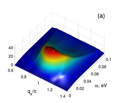
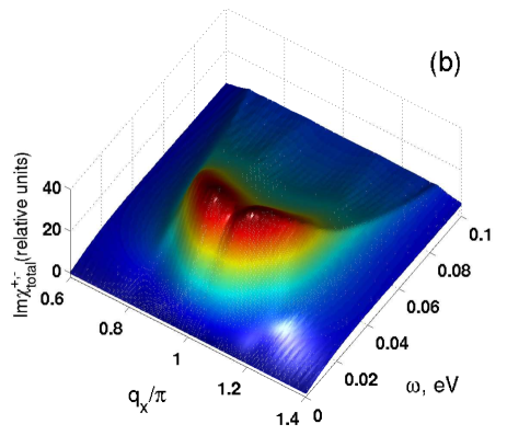
Figure 1: Calculated imaginary part of the spin susceptibility for the normal state (T=100K) near the wave vector $Q=(\pi,\pi)$ as a function of $\omega$ (in eV) and $q_{x}$ [$q_{y}=\pi$] for $\varGamma=6$meV (a) and that using Eq.(38) with $\varGamma_{1}=6meV$, $\varGamma_{2}=6meV$, $\xi=0.05\pi$. (b)

.

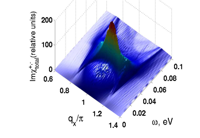
Figure 2: Calculated imaginary part of spin susceptibility for the superconducting state (T=10K) near the wave vector $Q=(\pi,\pi)$ as a function of $\omega$ (in eV) and $q_{x}$ for $q_{y}=\pi$.

The calculated imaginary part of susceptibility in the normal phase for $T=100K$ is shown in Fig. 1. The chosen parameters are: $J_{1}=100meV$, $\Delta_{sp}=0.18$, and $\varGamma=6meV$. Values $F_{1}=0.15$ and $F_{2}=-0.02$ was estimated using Eq (28) at $K_{1}=-0.2$, $K_{2}=0.04$ and $\delta=0.3$. Observe that the imaginary part of total susceptibility has a visible upward dispersion, which can be attributed to a magnon-like mode damped at high frequencies due to coupling to the itinerant carriers. Note that the visible dispersion of the spin excitations centered at the antiferromagnetic wave vector Q, is in contrast to that found within a simple RPA expressionreznik . There the spin excitations are almost structureless in the normal state and refer to the overdamped Stoner continuum. Another important feature is that the spin excitations remain commensurate despite the significant hole doping as shown in Fig.1(a). This is due to the fact that the spin excitations has a character of the almost localised magnetic modes which are less sensitive to the degree of the Fermi surface nesting. One has, however, to keep in mind that in our calculations we take $\varGamma=6meV$ as a constant. In principle in a real physical system this value may become momentum and frequency dependent. In particular, assuming the coupling of the quasiparticles to the spin excitations, the quaiparticle lifetime will become anisotropic as a function of the Fermi surface angle. Quasiparticles connected by the antiferromagnetic momentum will scatter stronger as compared to those located near the diagonal of the BZ. As a result, the imaginary part of the self-energy (which affects $\varGamma$) will be larger around the wave vector Q and is smaller away from it. To demonstrate this effect we approximate $\varGamma$ by a Lorenzian in the form

$$\varGamma(q)=\varGamma_{1}+\varGamma_{2}\frac{(\xi)^{2}}{(|q_{x}|-\pi)^{2}+(|q_{y}|-\pi)^{2}+(\xi)^{2}}.$$ (38)

where $\xi$ is a magnetic correlation length. As one sees the effect of q-dependence of the damping $\varGamma$ yields a dip in imaginary part of susceptibility at $(\pi,\pi)$ as shown in Fig.1(b) and to the incommensurate magnetic fluctuations.

In Fig. 2 we show the imaginary part of the spin susceptibility in the superconducting state with $d_{x^{2}-y^{2}}$-wave symmetry. Observer the strong renormalization of the entire spectrum of the spin excitations. As a consequence of the $d$-wave symmetry of the order parameter there is a resonance mode forming at energies well below $|\Delta_{\mathbf{k}}+\Delta_{\mathbf{k+Q}}|\sim 60$meV. Away from the antiferromagnetic momentum, the excitations shows the $X-$shape structure which appears only in the superconducting state. Due to the delicate balance between the spin-gap parameter $\Delta_{s}$ and the twice superconducting gap, $2\Delta_{0}$, the frequency position of the resonance peak in superconducting state is almost unchanged with regard to the normal state value. However, its position is still below the onset of particle-hole continuum which starts approximately at $2\Delta_{0}$. Taking the constant energy cuts of the excitations shown in Figs. 1 and 2 one finds that the results are very similar to those observed in inelastic neutron scattering in $YBa_{2}Cu_{3}O_{6.92}$ and $YBa_{2}Cu_{3}O_{6.97}$ (see Fig. 8) in P. Bourges Rev. bourge . Note that the calculated upward and downward dispersions shown in Fig. 2 look similar to those found experimentally in $YBa_{2}Cu_{3}O_{6.95}$ (see Fig. 3(c) in reznik ), (Fig. 5(a)-(b) in Ref. bourge ), $YBa_{2}Cu_{3}O_{6.85}$ (Fig. 4(a) in Ref. pailhes ), $YBa_{2}Cu_{3}O_{6.6}$ (Fig.5 in Ref. arai ), and $YBa_{2}Cu_{3}O_{6.5}$ (Fig. 5 in Ref.stock ). The coexistence of both downward and upward branches can be clearly seen in Fig. 2. While the downward dispersion refers to the itinerant component of the spin response and the evolution of $d$-wave gap on the Fermi surface, the upward dispersion originates mostly from magnon-like short-range antiferromagnetic fluctuations. Important to note here is that these dual features are obtained using the general expression for the spin susceptibility which accounts for both local and itinerant spin excitations.

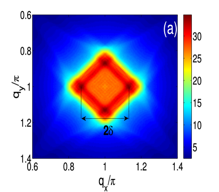
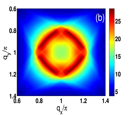
Figure 3: Intensity plot of the imaginary part of the susceptibility $Im\chi^{+,-}(\omega,q)$ around wave vector $Q=(\pi,\pi)$ for $\hbar\omega=40meV$ (a) and $\hbar\omega=60meV$ (b),$\varGamma=6meV$.

In Fig.3 we show the intensity plot of the imaginary part of the susceptibility $Im\chi^{+,-}(\omega,q)$ as a function of q around the wave vector $Q=(\pi,\pi)$ in the superconducting state for the energies above and below the resonance energy positions, $\omega_{res}$. Below $\omega_{res}$ in agreement with experimental observation reznik and RPA calculations eremin05 we have found quadratic in q downward dispersion with dominant peaks along the bond directions. The latter is due to fact that there is more phase space available for $(\pi,\pi+\delta)$ directions as they are closer to the resonance at $(\pi,\pi)$ than those at the diagonal wave vector at this energy. At the same time, the upward branch above $\omega_{res}$ has almost circular symmetry around $Q_{AF}$ which is the same as in the normal state and agrees with experimental observation reznik . In order to see the evolution of the incommensurability with the superconducting gap we plot $\Delta_{0}$ vs $2\delta/\pi$ in Fig. 4.

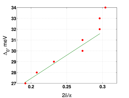
Figure 4: The incommensurability parameter, $2\delta/\pi$ plotted as a function of the superconducting gap amplitude $\Delta_{0}$. The red points refer to the calculated values using Eq. (29) and the solid line is a guide to the eye.

Observe that for increasing $\Delta_{0}$ the incommensurability parameter, $\delta$, computed for $\omega=40meV$ increases. This is an indication that the incommensurability for $\omega<\omega_{res}$ refers to the spin exciton dispersion which is connected to the magnitude of the superconducting gap. Namely, the increase of $\Delta_{0}$ shifts the position of the resonance peak to higher energies. For a given $\omega<\omega_{res}$ this increase implies that the itinerant spin excitations arises from the scattering of the quasiparticle states located at the Fermi surface points which are closer and closer to the diagonals of the BZ, i.e. smaller q_i (larger $2\delta$). Note that this observation is in direct correspondence with the result found previously in experimental data (see Fig. 25 in Ref. dai ). At certain point, when the resonance energy is large enough, the only electron-hole scattering available originates from the nodal points where the superconducting gap is zero. At this moment, the incommensurability starts to be independent on the $\Delta_{0}$, the effect clearly visible in Fig.4. This observation confirms the itinerant origin of the lower branch of the dispersion of the spin excitations. Note that the incommensurability of the spin excitations for $\omega>\omega_{res}$ is not sensitive to the magnitude of the superconducting gap as it arises from the localised magnetic excitations. In this case it remains a constant (not shown) independent on the size of the superconducting gap.

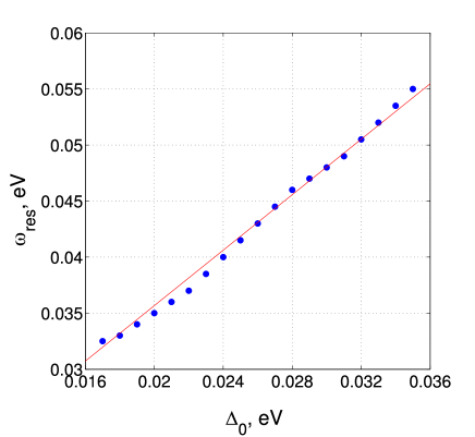
Figure 5: Calculated relationship between the resonance energy (in meV) and superconductivity gap $\Delta_{0}$.

In Fig.5 we show the relation between the resonance energy and superconductivity gap $\Delta_{0}$. Despite the fact that this observation is a direct consequence of the resonance being the spin exciton we show it here as it agrees fairly well with experimental data (see, for example, Fig. 26 in Ref. dai ).

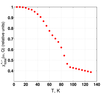
Figure 6: Temperature dependence of the resonance peak intensity.

Finally, in Fig.6 we show the calculated temperature dependence of the resonance peak using the temperature dependence of the gap
$\Delta(T)=\Delta_{0}\tanh\left(1.76\sqrt{T_{c}/T-1}\right)$ which was obtained previouslymayer ; eremin3 . The resonance peak intensity follows the temperature dependence of the superconducting gap. Above $T_{c}$ the resonance mode continuously evolves into paramagnon mode. We stress that the true resonance exists only below T_c and the excitations above T_c refers to the spectrum of the normal state. This result is in agreement with the experimental observation found in $YBa_{2}Cu_{3}O_{6.97}$ (see Fig.10 in Ref. bourge and also Fig.4(a) in Ref. bourge2 ).

At the end of this section we shortly summarize the differences between our results and those obtained earlier either in a conventional RPA scheme or within a memory functions formalism (MFF). As it was pointed out in previous RPA studies, see Ref. reznik , the conventional RPA scheme explains quite well the downward part of the dispersion of the spin excitation which originates in this case due to d-wave symmetry of the superconducting gap, but does not reproduce the upward one which should refer to the paramagnon dispersion. The origin of this is that the lifetime of the quasiparticles is not included within simple RPA. As a result, the paramagnons at higher energies are strongly damped due to a standard Landau damping mechanism. In our approach the Landau damping is suppressed by the kinematic ”molecular” field which originates from local no-double occupancy constraint. The constraint reduces the phase space available for the particle-hole continuum to form and suppresses then the Landau damping. As a result the upper paramagnon part of the dispersion is more visible.

At the same time the chains of equations of motion with a decoupling procedure employed by us and memory function formalism used by other groups are closely related. In the memory function formalism one decouples the exchange part of the Hamiltonian in fashion similar to ours. The resulting dispersion of the localized excitations is then again referred to the upward branch of the spin excitation seen in INS. To account for the superconductivity and presence of itinerant electrons, which give rise to the downward dispersion, one introduces the decoupling of the spin-excitation damping. This describes the decay of the spin excitation into an electron-hole pair. Here, superconductivity is introduced phenomenologically in the energy spectrum of the quasiparticles. One finds that the results for the spin excitations within memory function and equations of motion formalism are quite similar, see Refs. sherman ; prelovsek ; vladimirov . However, we believe that our approach dealing with the chains of equations of motion has certain advantages. In particular, it allows to reproduce wider range of experimental data on INS for $T<T_{c}$ (also including NMR and ARPES data) and, most importantly, we are able to describe both upward and downward dispersions (see Fig. 3) within a single analytical expression. Here, the origin of various terms have a transparent physics meaning and the parameters of the quasiparticle dispersion and the spin excitation spectrum are computed self-consistently.

5 Concluding remarks

To conclude, in this paper we present the analysis of the spin response in the superconducting cuprates taking into account both the local and the itinerant component of the magnetic excitations coupled in a self-consistent manner. The numerical results show that the obtained expression for the spin susceptibility, Eq. (29), reproduces well the characteristic features of the experimental data in $YBa_{2}Cu_{3}O_{6+y}$ compounds near the optimal doping including the dispersion of the spin excitations in the normal and superconducting state as well its frequency and temperature dependence. While the structure of the spin excitations in the normal state can be attributed to the overdamped localised magnetic modes, the strong feedback of the $d$-wave superconductivity on the itinerant electrons reveals the formation of the spin exciton with the characteristic downward dispersion of the spin excitations in the superconducting state. In addition, the high energy spin excitations still originates from the localised excitations. Remarkable that both modes merge at the $\omega_{res}$ which is a result of the single pole structure at Q in Eq. (29). Our analytical results suggests the dual character of the spin response even in the optimally doped cuprates.

The authors acknowledge A. Barabanov, M. Mali, P.F. Meier, A. Mikheenkov, N. Plakida, J. Roos, for useful remarks and discussions. This work was supported in part by the Russian Foundation for Basic Research, Grant 09-02-00777-a and Swiss National Science Foundation, Grant IZ73Z0 128242.

References

- (1) P.W. Anderson, Science 235, 1196 (1987); F.C. Zhang, T.M. Rice, Phys. Rev. B 37, 3759 (1988); G. Baskarn, Z. Zou and P.W. Anderson, Solid State Commun. 63, 973 (1987); S.A. Kivelson, E. Fradkin and V.J. Emery, Nature 393, 550 (1998); M. Vojta and S. Sachdev, Phys. Rev. Lett. 83, 3916 (1999); S.R. White and D.J. Scalapino, Phys. Rev. B 61, 6320 (2000); T. Senthil and M.P.A. Fisher, Phys. Rev. B 64, 214511 (2001).
- (2) P. Monthoux and D. Pines, Phys. Rev. B 49, 4261 (1994); C. Castellani, C. DiCastro and M. Grilli, Phys. Rev. Lett. 75, 4650 (1995); S. Chakravarty, R. Laughlin, D.K. Morr and C. Nayak, Phys. Rev. B 63, 094503 (2001); A. Abanov, A.V. Chubukov and J. Schmalian, Adv. Phys. 52, 119 (2003); W. Metzner, D. Rohe and S. Andergassen, Phys. Rev. Lett. 91, 066402 (2003); M.R. Norman, D. Pines and C. Kallin, Adv. Phys. 54, 715 (2005); T.A. Maier, D. Poilblanc and D.J. Scalapino, Phys. Rev. Lett. 100, 237001 (2008); M. Ossadnik, C. Honerkamp, T.M. Rice and M. Sigrist, Phys. Rev. Lett. 101, 256405 (2008).
- (3) T. Dahm, D. Manske, L. Tewordt, Phys. Rev. B 58, 12454 (1998); D. Manske, I. Eremin, and K. H. Bennemann, Phys. Rev. B 63, 054517 (2001).
- (4) F. Onufrieva and J. Rossat-Mignod, Phys. Rev. B 52, 7572 (1999); F. Onufrieva and P. Pfeuty, Phys. Rev. B 65, 054515 (2002).
- (5) M.R. Norman, Phys. Rev. B 63, 092509 (2000); M. Eschrig and M.R. Norman, Phys. Rev. B 67, 144503 (2003).
- (6) I. Eremin, D.K. Morr, A.V. Chubukov, K.H. Bennemann, and M.R. Norman, Phys. Rev. Lett. 94, 147001 (2005).
- (7) Ar. Abanov, A. V. Chubukov, M. Eschrig, M. R. Norman, and J. Schmalian, Phys. Rev. Lett. 89, 177002 (2002).
- (8) A. Schnyder, A. Bill, C. Mudry, R. Gilardi, H.M.Ronnow, and J. Mesot, Phys. Rev. B 70, 214511 (2004).
- (9) H. Shimahara, S. Takada, J. Phys. Soc. Jpn. 61, 989 (1992).
- (10) S. Winterfeld, D. Ihle, Phys. Rev. B 58, 9402 (1998); ibid Phys. Rev. B 59, 6010 (1999).
- (11) A. Yu. Zavidonov, D. Brinkmann, Phys. Rev. B 58, 12486 (1998).
- (12) A. Sherman and M. Schreiber, Phys. Rev. B 68, 094519 (2003); A. Sherman and M. Schreiber, Eur. Phys. Jour. B 32, 203 (2003).
- (13) I. Sega, P. Prelovsek, Phys. Rev. B 73, 092516 (2006); I. Sega, P. Prelovsek, J. Bonca. Phys. Rev. B 68, 054524 (2003); P. Prelovsek, I. Sega, J. Bonca. Phys. Rev. Lett. 92, 027002 (2004); P. Prelovsek, I. Sega Phys. Rev. B 74, 214501 (2006).
- (14) H. Yamase, and W. Metzner, Phys. Rev. B 73, 214517 (2006).
- (15) A.V. Mikheenkov and A.F. Barabanov, Zh. Eksp. Theor. Fiz. 132, 392 (2007) [JETP 105, 347 (2007)].
- (16) A.A. Vladimirov, D. Ihle and N.M. Plakida, Phys. Rev. B 80, 104425 (2009); ibid. Phys. Rev. B 83, 024411 (2011).
- (17) L.M. Roth, Phys. Rev. B 184, 451 (1969).
- (18) J. Beenen and D.M. Edwards, Phys. Rev. B 52, 13636 (1995).
- (19) N.M. Plakida, R. Hayn, and J.-L. Richard, Phys. Rev. B 51, 16599 (1995).
- (20) P.W. Anderson, P.A. Lee, M. Randeria, T.M. Rice, N. Trivedi, F.C. Zhang, J Phys. Condens. Mat., R 754 (2004).
- (21) M.V. Eremin, A.A. Aleev, and I.M. Eremin, Pis’ma Zh. Eksp. Teor. Fiz. 84(3), 197 (2006) [JETP Lett. 84(3),167 (2006)].
- (22) M.V. Eremin, A.A. Aleev, and I.M. Eremin, Zh. Eksp. Teor. Fiz. 133(4), 862 (2008) [JETP 106(4), 752 (2008)].
-
(23)
M. I. Auslender, V.Yu. Irkhin and M.I.
Katsnelson, J. Phys. C: Solid State Phys. 21, 5521-5537 (1988);
J. J. Field, J. Phys. C: Solid State Phys. 5, 664-675 (1972); J. Hubbard and K. P. Jain, J.Phys. C (Proc. Phys. Soc. ) ser. 2, vol. 1, 1650-1657 (1968). - (24) T. Mayer, M. Eremin, I. Eremin and P.F. Meier, J. Phys.: Condens. Matter 19, 116209 (2007).
- (25) M.V. Eremin, I.A. Larionov, and I.E. Lyubin, J. Phys. Condens. Matter 22, 185704-185709 (2010).
- (26) D. Reznik, J.-P. Ismer, I. Eremin, L. Pintschovius, T. Wolf, M. Arai, Y. Endoh, T. Masui, and S. Tajima, Phys. Rev. B 78, 132503 (2008).
- (27) P. Bourges, in The Gap Symmetry and Fluctuations in High Temperature Superconductors, edited By J. Bok, G. Deutscher, D. Pavuna, and S.A. Wolf (Plenum, New York, 1998); V. Hinkov and B. Keimer, A. Ivanov, P. Bourges and Y. Sidis, C.D. Frost, arXiv: 1006.3278v1 [cond-mat.supr-con] (unpublished).
- (28) D. Reznik, P. Bourges, L. Pintschovius, Y. Endoh, Y. Sidis, T. Masui and S. Tajima, Phys. Rev. Lett. 93, 207003 (2004).
- (29) S. Pailhès, Y. Sidis, P. Bourges, V. Hinkov, A. Ivanov, C. Ulrich, L. P. Regnault, and B. Keimer, Phys. Rev. Lett. 93, 167001 (2004).
- (30) M. Arai, T. Nishijima, Y. Endoh, T. Egami, S. Tajima, K. Tomimoto, Y. Shiohara, M. Takahashi, A. Garrett, and S. M. Bennington, Phys. Rev. Lett. 83, 608 (1999).
- (31) C. Stock, W.J.L. Buyers, R.A. Cowley, P.S. Clegg, R. Coldea, C.D. Frost, R. Liang, D. Peets, D. Bonn, W.N. Hardy, and R.J. Birgeneau, Phys. Rev. B 71, 024522 (2005).
- (32) Pengcheng Dai, H.A. Mook, R.D. Hunt, F. Dog̃an, Phys. Rev. B 63, 054525 (2001).
- (33) P. Bourges, Y. Sidis, H.F. Fong, L.P. Regnault, J. Bossy, A. Ivanov, B. Keimer, Science 288, 1234 (2000).