$90^{\circ}$ Ferroelectric Domains in PbTiO₃: Experimental Observation and Molecular Dynamics Simulations

Abstract

We report observation of $90^{\circ}$ ferroelectric domain structures in transmission electron microscopy (TEM) of epitaxially-grown films of PbTiO₃. Using molecular dynamics (MD) simulations based on first-principles effective Hamiltonian of bulk PbTiO₃, we corroborate the occurance of such domains showing that it arises as metastable states only in cooling simulations (as the temperature is lowered) and establish characteristic stability of $90^{\circ}$ domain structures in PbTiO₃. In contrast, such domains do not manifest in similar simulations of BaTiO₃. Through a detailed analysis based on energetics and comparison between PbTiO₃ and BaTiO₃, we find that $90^{\circ}$ domain structures are energetically favorable only in the former, and the origin of their stability lies in the polarization-strain coupling. Our analysis suggests that they may form in BaTiO₃ due to special boundary condition and/or defect-related inhomogeneities.

I Introduction

Ferroelectric transitions in perovskite oxides, such as BaTiO₃, are fluctuation driven first-order phase transitions, and hence a state with spatially fluctuating order parameter can readily form as a result of certain mechanical and electric boundary conditionsKumar and Waghmare (2010). A common example of such a state is the one with domains of ferroelectric polarization with different symmetry equivalent orientations of order parameter that are separated by domain walls. Indeed, many properties of perovskite ferroelectrics depend on such domain structure, and it is being increasingly relevant at nano-scaleSchilling et al. (2009); Luk’yanchuk et al. (2009a); Fong et al. (2004); Paul et al. (2007). Naturally, the properties of a domain wall or an interface between adjacent ferroelectric domains depend on (a) symmetries and structural details of ferroelectric phases and (b) microscopic couplings responsible for the ferroelectric phase transition.

Perovskite oxides such as BaTiO₃ and PbTiO₃ are representative ferroelectric materials, although are quite different from each other in terms of their phase transitions. While PbTiO₃ undergoes a single strongly first order phase transition from cubic to tetragonal structure as temperature is lowered, BaTiO₃ exhibits a sequence of three relatively weaker first-order phase transitions. A paraelectric phase of BaTiO₃ with cubic structure transforms into a tetragonal ferroelectric phase at a Curie temperature, 393 K. Further cooling produces sudden changes from a tetragonal phase to an orthorhombic phase at 278 K and from an orthorhombic phase to a rhombohedral phase at 203 KShirane and Takeda (1951); von Hippel (1950). On the other hand, PbTiO₃ exhibits a phase transition from a paraelectric cubic phase to a ferroelectric tetragonal phase at $T_{\rm C}=763$ K and remains tetragonal down to 0 KShirane et al. (1950, 1956, 1955).

While the domain structures in ferroelectrics have been revealed experimentallyvon Hippel (1950); Schilling et al. (2006); Rodriguez et al. (2010); Matsumoto et al. (2008); Luk’yanchuk et al. (2009b); Fousek and Safranko (1965); Tanaka and Honjo (1964); Tanaka et al. (1962); Matsumoto and Okamoto (2011); Nakaki et al. (2008, 2007); Lee and Baik (2006); Aoyagi et al. (2011); Kiguchi et al. (2011); Stemmer et al. (1995); Hsu and Raj (1995), detailed in situ experimental analysis of the domains and domain walls is quite challenging and the temperature dependence of dynamics of domain structure is not well understood. In the case of PbTiO₃, experimental studies of domains are further more difficult as the sample needs to be heated over its high transition temperature $T_{\rm C}=763$ K and such heating leads to evaporation of Pb ions changing the composition of the sampleGerson (1960).

Ferroelectric phase transitions in perovskite oxides in bulk and thin film have been investigated by computer simulations such as phase-field methodLi et al. (2001), Monte Carlo simulationsZhong et al. (1995), and molecular dynamics (MD) simulationsWaghmare et al. (2003). Recently, Nishimatsu et al. have developed a fast and versatile MD simulator of ferroelectrics based on first-principles effective HamiltonianNishimatsu et al. (2008) which can be used in systematic studies of bulk as well as thin films. They have studied BaTiO₃ bulk and thin-film capacitors and obtained results showing good agreement with experiments. Their MD simulations of BaTiO₃ under periodic boundary condition (PBC) for bulk did not show any domain structures, as there is no depolarization field in the PBC of bulk. Simulations of thin-film of BaTiO₃ only show $180^{\circ}$ domain structuresNishimatsu et al. (2008), though $90^{\circ}$ domain structures are widely seen in experimentsSchilling et al. (2006); Matsumoto et al. (2008). One of the advantages of MD simulations compared to Monte Carlo simulations is its ability to simulate time-dependent dynamical phenomena, e.g. MD simulation can be used to study the evolution of ferroelectric domains as a function of time during heating-up and cooling-down simulations.

In this paper, we report heating-up and cooling-down molecular-dynamics (MD) simulations of bulk PbTiO₃ to understand our observation of $90^{\circ}$ domain structures in epitaxially-grown sample of PbTiO₃. In Sec. II, we present experimental details for the sample preparation and we show a transmission electron microscope (TEM) image of $90^{\circ}$ domain structure in PbTiO₃ film. We briefly explain the first-principles effective Hamiltonian and details of MD simulations in Sec. III and we present our results and analysis of heating-up and cooling-down MD simulations in Sec. IV. We finally summarize our work and conclusions in Sec. V.

II Experimental Details and Observations

II.1 Sample preparation and Methods of TEM

An epitaxial PbTiO₃ thick film, with film thicknesses of about 1200 nm, was grown on the SrRuO₃/SrTiO₃ substrate at 873 K by pulsed metal organic chemical vapor deposition (pulsed-MOCVD) method. SrRuO₃ was deposited on (100) SrTiO₃ by rf-magnetron sputtering method. The detail of film preparation technique is described elsewhereNagashima and Funakubo (2000); Nagashima et al. (2000). The TEM specimens were prepared with focused ion beam (FIB) micro-sampling technique. Damage layers, introduced during FIB microfabrication, were removed by low-energy Ar ion milling at 0.3 kV. JEM-2000EXII was used for TEM observations. TEM observations were performed at room temperature.

II.2 Observed TEM image

In Fig. 1, we show a bright field TEM image of a PbTiO₃ thick film, taken with the incident electron beam parallel to the [100] axis of the PbTiO₃. The inset in the image is the corresponding selected-area electron diffraction pattern. This bright-field TEM image is taken with the scattering vector $g_{0\bar{1}\bar{1}}$ excited. Here, $a$- and $c$-domains are those with polarization along $a$ and $c$ axes of the PbTiO₃ parallel and perpendicular to the substrate, respectively. This domain configuration is typical and very commonly seen for tetragonal PbTiO₃ films. The domain size is about 50-200 nm. Such $90^{\circ}$ domain configurations, similar to that in Fig. 1, have been also observed in BaTiO₃Schilling et al. (2006); Matsumoto et al. (2008). Boundaries between a- and c-domains are seen as black lines, as the TEM sample is slightly tilted. From this image, we can not discuss the width of domain walls between a- and c-domain. High-resolution TEM observation has revealed that the width of $90^{\circ}$ domain walls is $1.0\pm 0.3$ nmStemmer et al. (1995). To this end, high-resolution TEM observation was conducted in order to reveal the width of domain walls between a- and c-domain. Fig. 2 shows the high-resolution TEM image of PbTiO₃ film, indicating that the width of domain walls is corresponding to 1 or 2 unit cells.

Before our computational study, it should be worth mentioning that $90^{\circ}$ domains have been often observed in both BaTiO₃ and PbTiO₃, and are both ferroelectric and ferroelastic in nature. Typically, $90^{\circ}$ domains are formed in epitaxial ferroelectric and ferroelastic films in order to relax the strain resulting from lattice mismatch with the substrate at and below $T_{\rm C}$.Pompe et al. (1993); Speck and Pompe (1994) They nucleate at misfit dislocations formed above $T_{\rm C}$. Their growth is accompanied with the introduction of the additional dislocation perpendicular to the misfit dislocations and the dissociation of the dislocations into two pairs of partial dislocations around an anti-phase boundaryKiguchi et al. (2011).

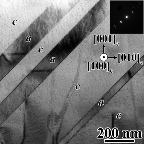
Figure 1: A bright-field TEM image of a PbTiO₃ thick film taken with an electron incident parallel to the [100] of PbTiO₃. Scripts a and c in this figure denote a-domain and c-domain, respectively.

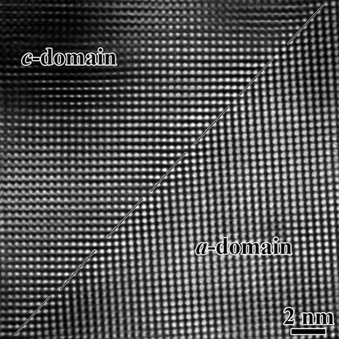
Figure 2: A high-resolution TEM image of a PbTiO₃ thick film taken with an electron incident parallel to the [100] of PbTiO₃. The $90^{\circ}$ domain boundary is shown by the chain line.

III Molecular Dynamics Simulations

III.1 Effective Hamiltonian

Heating-up and cooling-down molecular-dynamics (MD) simulations are performed using first-principles effective Hamiltonian King-Smith and Vanderbilt (1994); Zhong et al. (1995); Waghmare et al. (2003); Nishimatsu et al. (2008, 2010),

$$H^{\rm eff}=\frac{M^{*}_{\rm dipole}}{2}\sum_{\bm{R},\alpha}\dot{u}_{\alpha}^{2}(\bm{R})+\frac{M^{*}_{\rm acoustic}}{2}\sum_{\bm{R},\alpha}\dot{w}_{\alpha}^{2}(\bm{R})\\ +V^{\rm self}(\{\bm{u}\})+V^{\rm dpl}(\{\bm{u}\})+V^{\rm short}(\{\bm{u}\})\\ +V^{\rm elas,\,homo}(\eta_{1},\ldots\!,\eta_{6})+V^{\rm elas,\,inho}(\{\bm{w}\})\\ +V^{\rm coup,\,homo}(\{\bm{u}\},\eta_{1},\ldots\!,\eta_{6})+V^{\rm coup,\,inho}(\{\bm{u}\},\{\bm{w}\})~{},$$ (1)

where $\bm{u}=\bm{u}(\bm{R})$ and $\bm{w}=\bm{w}(\bm{R})$ are, respectively, the local dipolar displacement vector and the local acoustic displacement vector of the unit cell at $\bm{R}$ in a simulation supercell. $\alpha(=x,y,z)$ is the Cartesian directions. Braces $\{\}$ denote a set of $\bm{u}$ or $\bm{w}$ in the supercell. $\eta_{1},\ldots\!,\eta_{6}$ are the homogeneous strain components. $M^{*}_{\rm dipole}$ and $M^{*}_{\rm acoustic}$ are the effective masses for $\bm{u}$ and $\bm{w}$, therefore, first two terms in Eq. (1) are kinetic energies of them.

$V^{\rm self}$, $V^{\rm dpl}$, $V^{\rm short}$, $V^{\rm elas,\,homo}$, $V^{\rm elas,\,inho}$, $V^{\rm coup,\,homo}$, and $V^{\rm coup,\,inho}$ are a local-mode self-energy, a long-range dipole-dipole interaction, a short-range interaction, a homogeneous elastic energy, an inhomogeneous elastic energy, a couping between $\{\bm{u}\}$ and $\eta_{1},\ldots\!,\eta_{6}$, and a couping between $\{\bm{u}\}$ and $\{\bm{w}\}$, respectively. More detailed explanation of symbols in the effective Hamiltonian can be found in Refs. Nishimatsu et al., 2008 and Nishimatsu et al., 2010. We take all the parameters of the first-principles effective Hamiltonian for PbTiO₃ from the earlier workWaghmare and Rabe (1997). However, the form of the effective Hamiltonian we use in our simulationsNishimatsu et al. (2008, 2010) is slightly different from the one used to get the parameters in Ref. Waghmare and Rabe, 1997. The new parameters can be easily derived from the previous ones. We list values of all the parameters used in our simulations and how they are related to the previous work Waghmare and Rabe (1997) in Table 1.

Table 1: The parameters of first-principles effective Hamiltonian for PbTiO₃ used in our simulations are given in the second column and how these parameters are related with the parameters in the previous workWaghmare and Rabe (1997) are shown in the third column.

parameters	value	relation
$a_{0}$ [Å]	3.969	a0
$B_{11}$ [eV]	117.9	$C_{11}$
$B_{12}$ [eV]	51.6	$C_{12}$
$B_{44}$ [eV]	137.0	$C_{44}$
$B_{1xx}$ [eV/Å2]	$-114.02$	2($g_{0}$+$g_{0}$)
$B_{1yy}$ [eV/Å2]	$-13.67$	2$g_{0}$
$B_{4yz}$ [eV/Å2]	$-22.67$	$g_{2}$
$\alpha$ [eV/Å4]	$27.83$	$B+C$
$\gamma$ [eV/Å4]	$-34.48$	$-2C$
$k_{1}$ [eV/Å6]	$-42.42$	$D$
$k_{2}$ [eV/Å6]	0
$k_{3}$ [eV/Å6]	0
$k_{4}$ [eV/Å8]	156.43	$E$
$m^{*}$ [amu]	100.0
$Z^{*}$ [e]	10.02	$Z^{*}$
$\epsilon_{\infty}$	8.24	$\epsilon_{\infty}$
$\kappa_{2}$[eV/Å2]	1.170	$A$
$j_{1}$ [eV/Å2]	$-1.355$	$2a_{T}$
$j_{2}$ [eV/Å2]	$4.986$	$2a_{L}$
$j_{3}$ [eV/Å2]	$0.222$	$b_{l}+b_{t1}$
$j_{4}$ [eV/Å2]	$-0.018$	$2b_{t2}$
$j_{5}$ [eV/Å2]	$0.398$	$b_{l}-b_{t1}$
$j_{6}$ [eV/Å2]	$-0.083$	$\frac{2(c_{l}+2c_{t})}{3}$
$j_{7}$ [eV/Å2]	$-0.204$	$\frac{2(c_{l}-2c_{t})}{3}$

III.2 Simulation Details

Heating-up and cooling-down MD simulations are performed with our original MD code feram (http://loto.sourceforge.net/feram/). Details of the code can be found in Ref. Nishimatsu et al., 2008. Temperature is kept constant in each temperature step in the canonical ensemble using the Nosé-Poincaré thermostat.Bond et al. (1999) This simplectic thermostat is so efficient that we can set the time step to $\Delta t=2$ fs. In our present MD simulations, we thermalize the system for 20,000 time steps, after which we average the properties for 20,000 time steps. We used a supercell of system size $N=L_{x}\times L_{y}\times L_{z}=32\times 32\times 32$ and small temperature steps in heating-up ($+1$ K/step) and cooling-down ($-1$ K/step) simulations. The heating-up simulation from 100 K to 900 K is started from an $z$-polarized initial configuration generated randomly: $\langle u_{x}\rangle=\langle u_{y}\rangle=0$, $\langle u_{z}\rangle=0.33~{}{\rm\AA}$, $\langle u_{x}^{2}\rangle-\langle u_{x}\rangle^{2}=\langle u_{y}^{2}\rangle-\langle u_{y}\rangle^{2}=(0.045~{}{\rm\AA})^{2}$, and $\langle u_{z}^{2}\rangle-\langle u_{z}\rangle^{2}=(0.021~{}{\rm\AA})^{2}$, where brackets denote $\bm{R}$-average in supercell $\langle u_{\alpha}\rangle=\frac{1}{N}\sum_{\bm{R}}u_{\alpha}(\bm{R})$. The cooling-down one from 900 K to 100 K is started from random paraelectric initial configuration: $\langle u_{x}\rangle=\langle u_{y}\rangle=\langle u_{z}\rangle=0$ and $\langle u_{\alpha}^{2}\rangle-\langle u_{\alpha}\rangle^{2}=(0.15~{}{\rm\AA})^{2}$.

IV Results and Discussion

From the temperature dependence of averaged lattice constants (shown in Fig. 3), a tetragonal-to-cubic ferroelectric-to-paraelectric phase transition is clearly observed in the heating-up simulation at 677 K. However, a strange behavior in lattice constants is found in the cooling-down simulation at T=592 K. The average temperature of these two transition temperatures (634 K) is in good agreement with the earlier Monte Carlo simulations and slightly lower than the experimental value $T_{\rm C}=763$ K. Indeed, the observation of an orthorhombic phase during cooling-down simulations is intriguing.

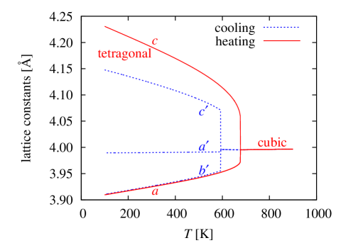
Figure 3: (Color online) Simulated temperature dependence of lattice constants of PbTiO₃ in heating-up (red solid lines) and cooling-down (blue dashed lines) molecular-dynamics simulations.

To understand this interesting behaviour of lattice constants in cooling-down simulations, we perform a detailed analysis of the configurations (snapshots) during our MD simulations. From a snapshot of dipoles in the supercell (shown in Fig. 4), we find that the apparently orthorhombic nature of the phase is due to a $90^{\circ}$ domain structure. Although the 4 unit cell $=1.6$ nm of the domain size is much smaller than experimentally observed ones as shown in Sec. II.2, the width of a simulated domain wall estimated to be $\sim~{}1$ unit cell is in good agreement with our experiment. Each domain has the $a=b<c$ tetragonal structure of PbTiO₃, but their average value in whole crystal gives smaller $c^{\prime}$ than $c$ and larger $a^{\prime}$ than $a$. The lattice constant $b^{\prime}$ has almost the same values as $a$, because the polar directions of two kind of domains are perpendicular to the $b^{\prime}$-axis. It should be noted that this domain structure is found in MD simulations in bulk under periodic boundary condition (PBC), but we have not simulated thin films. Under the PBC, there is no depolarization field inside the bulk. Moreover, this domain structure can be easily reproduced in cooling-down simulations from any random paraelectric initial configurations and any seeds for the pseudo random number generatorMarsaglia and Tsang (2004). There was no evidence for such unusual behavior in simulations of bulk BaTiO₃ Nishimatsu et al. (2008, 2010).

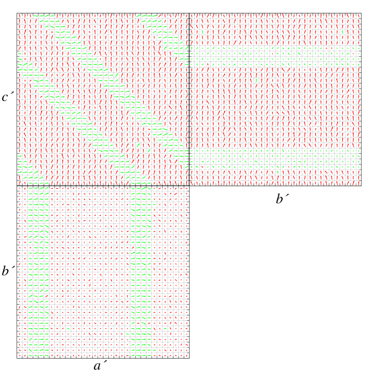
Figure 4: (Color online) Snapshot of three “sides” of the $32\times 32\times 32$ supercell at $T=300$K in a cooling-down simulation of PbTiO₃. Dipole moments of each site are projected onto the side planes and indicated with arrows. Dipoles of $u_{z}>0.2$Å are indicated with red color. Dipoles of $u_{z}\leq 0.2$Å are indicated with green. Crystalline directions are indicated with $a^{\prime}$, $b^{\prime}$, and $c^{\prime}$ as indicated in Fig. 3.

To understand the reason of stability of the $90^{\circ}$ domain structure seen here, even in bulk PbTiO₃, we compare “total energy surfaces” between single and $90^{\circ}$ domain structures. The total energy surface of single domain structure with $[001]$ polarization is the same as in Refs. King-Smith and Vanderbilt, 1994 and Nishimatsu et al., 2008. For the total energy surface of $90^{\circ}$ domain structure, we focus on a snapshot of the supercell at 300K shown in Fig. 4 and represent it with $\{\bm{u}_{90^{\circ}\!,300{\rm K}}(\bm{R})\}$. We now obtain a sequence of configurations by multiplying a factor $\frac{u}{\langle u\rangle_{90^{\circ}\!,300{\rm K}}}$ for all $\bm{R}$

$$\bm{u}(\bm{R})=\frac{u}{\langle u\rangle_{90^{\circ}\!,300{\rm K}}}\bm{u}_{90^{\circ}\!,300{\rm K}}(\bm{R})~{},$$ (2)

and compute total energy as a function of $u$, where $\langle u\rangle_{90^{\circ}\!,300{\rm K}}$ is the averaged length of dipoles in the 300 K snapshot

$$\langle u\rangle_{90^{\circ}\!,300{\rm K}}=\frac{1}{N}\sum_{\bm{R}}|\bm{u}_{90^{\circ}\!,300{\rm K}}(\bm{R})|=0.32~{}{\rm\AA}~{}.$$ (3)

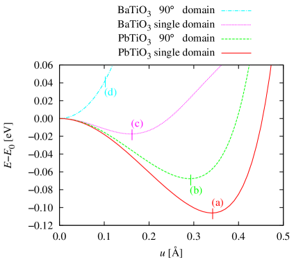
Figure 5: (Color online) Calculated total energy surfaces for PbTiO₃ single domain (solid line), PbTiO₃ $90^{\circ}$ domain (dashed line), BaTiO₃ single domain (dotted line), and BaTiO₃ $90^{\circ}$ domain (chain line).

Calculated total energy surfaces of single and $90^{\circ}$ domain structures for PbTiO₃ are shown in Fig. 5 with solid and dashed lines, respectively. For comparison, those for BaTiO₃ are also plotted assuming the same $90^{\circ}$ domain structure by using the set of parameters in $H^{\rm eff}$ listed in Ref. Nishimatsu et al., 2010. While the $90^{\circ}$ domain structure of PbTiO₃ exhibits a minimum at $u\neq 0$, that of BaTiO₃ costs energy. This is why the $90^{\circ}$ domain structures can be found in simple cooling-down simulations of PbTiO₃, but not in those of BaTiO₃.

Minima are indicated with (a)–(c) in Fig. 5. To uncover the origin of this contrasting behaviour, interaction energy terms at the minimums are listed in TABLE 2. For the BaTiO₃, because there is no minimum, interaction energies of configuration at (d) in Fig. 5 (of $u=0.10$ Å) are listed.

Table 2: Comparison of interaction energies $V^{i}$ in the effective Hamiltonian of Eq. (1) for two kinds of domain states of PbTiO₃ and BaTiO₃. $V^{\rm harmonic}$ is the sum of $V^{\rm dpl}$, $V^{\rm short}$, and the harmonic terms in $V^{\rm self}$. $V^{\rm unharmonic}$ is the unharmonic terms in $V^{\rm self}$. Unit of energy is eV.

$x$ of	PbTiO3	PbTiO3		BaTiO3	BaTiO3
interaction	(a) single	(b) $90^{\circ}$		(c) single	(d) $90^{\circ}$
energy $V^{x}$	domain	domain	$\Delta V^{i}$	domain	domain	$\Delta V^{i}$
harmonic	$-0.22106$	$-0.14393$	$+0.07713$	$-0.03886$	$0.03541$	$+0.07427$
unharmonic	$0.33435$	$0.17249$	$-0.16186$	$0.04754$	$0.00695$	$-0.04059$
elas,homo	$0.21946$	$0.04441$	$-0.17505$	$0.02609$	$0.00131$	$-0.02478$
elas,inho	$0.00000$	$0.05171$	$+0.05171$	$0.00000$	$-0.00262$	$-0.00262$
coup,homo	$-0.43891$	$-0.08881$	$+0.35010$	$-0.05218$	$0.00089$	$+0.05307$
coup,inho	$0.00000$	$-0.10342$	$-0.10342$	$0.00000$	$-0.00178$	$-0.00178$
total	$-0.10616$	$-0.06755$	$+0.03861$	$-0.01741$	$0.04016$	$+0.05757$
$u$ [Å]	0.34	0.29		0.16	0.10

From TABLE 2, It is clear that the energy losses in $V^{\rm harmonic}$, $V^{\rm elas,\,inho}$, and $V^{\rm coup,\,homo}$ in forming the $90^{\circ}$ domain structure in PbTiO₃ are compensated by the energy gains in $V^{\rm unharmonic}$, $V^{\rm elas,\,homo}$, and $V^{\rm coup,\,inho}$. In contrast, such recovery is not sufficient in BaTiO₃ to form a $u\neq 0$ minimum or non trivial 90^∘ domain structures. In stabilization of the 90^∘ domain structures in PbTiO₃, our analysis conclusively highlights the role of two microscopic interactions: (a) lower elastic energy cost arising from the smaller strain from compensation along $c$ and $a$ axis, and (b) inhomogeneous (local) strain coupling with polarization at the domain wall. The latter does not contribute much to transition behavior in the bulk, but has rather significant impact on the properties of domain wall. Noting that a $90^{\circ}$ domain structure is not energetically favorable in BaTiO₃ simulated as a perfect bulk crystal and coupling of soft modes with higher energy modes is weak, we believe that the experimentally observed $90^{\circ}$ domain structures in BaTiO₃ is most likely due to inhomogeneities in the samples and/or the specific electric and mechanical boundary conditions.

V Summary

In this article, TEM observation of PbTiO₃ thick films revealed $90^{\circ}$ domain structures, which have been often observed in BaTiO₃. The domain size perpendicular to domain boundaries was 50–200 nm. The width of domain wall was corresponding to 1 or 2 unit cell.

We also have performed heating-up and cooling-down MD simulations of PbTiO₃. In cooling-down simulation, $90^{\circ}$ domain structure is found to form spontaneously. By comparing “total energy surfaces” of single and $90^{\circ}$ domain structures, we understand that a $90^{\circ}$ domain structure is metastable in bulk PbTiO₃, but not in bulk BaTiO₃. The origin of this contrast is traced to significantly larger polarization-stran coupling in PbTiO₃. Hence, while $90^{\circ}$ domain structures can form spontaneously in PbTiO₃, they seem to arise in BaTiO₃ mostly from special boundary conditions and/or defect-related inhomogeneities.

References

- Kumar and Waghmare (2010) A. Kumar and U. V. Waghmare, Phys. Rev. B 82, 054117 (2010).
- Schilling et al. (2009) A. Schilling, D. Byrne, G. Catalan, K. G. Webber, Y. A. Genenko, G. S. Wu, J. F. Scott, and J. M. Gregg, Nano Letters 9, 3359 (2009), pMID: 19591494.
- Luk’yanchuk et al. (2009a) I. A. Luk’yanchuk, A. Schilling, J. M. Gregg, G. Catalan, and J. F. Scott, Phys. Rev. B 79, 144111 (2009a).
- Fong et al. (2004) D. D. Fong, G. B. Stephenson, S. K. Streiffer, J. A. Eastman, O. Auciello, P. H. Fuoss, and C. Thompson, Science 304, 1650 (2004).
- Paul et al. (2007) J. Paul, T. Nishimatsu, Y. Kawazoe, and U. V. Waghmare, Phys. Rev. Lett. 99, 077601 (2007).
- Shirane and Takeda (1951) G. Shirane and A. Takeda, J. Phys. Soc. Jpn. 6, 128 (1951).
- von Hippel (1950) A. von Hippel, Rev. Mod. Phys. 22, 221 (1950).
- Shirane et al. (1950) G. Shirane, S. Hoshino, and K. Suzuki, Phys. Rev. 80, 1105 (1950).
- Shirane et al. (1956) G. Shirane, R. Pepinsky, and B. Frazer, Acta Crystallogr. 9, 131 (1956).
- Shirane et al. (1955) G. Shirane, R. Pepinsky, and B. Frazer, Phys. Rev. 97, 1179 (1955).
- Schilling et al. (2006) A. Schilling, T. B. Adams, R. M. Bowman, J. M. Gregg, G. Catalan, and J. F. Scott, Phys. Rev. B 74, 024115 (2006).
- Rodriguez et al. (2010) B. J. Rodriguez, L. M. Eng, and A. Gruverman, Appl. Phys. Lett. 97, 042902 (2010).
- Matsumoto et al. (2008) T. Matsumoto, M. Koguchi, K. Suzuki, H. Nishimura, Y. Motoyoshi, and N. Wada, Appl. Phys. Lett. 92, 072902 (2008).
- Luk’yanchuk et al. (2009b) I. A. Luk’yanchuk, A. Schilling, J. M. Gregg, G. Catalan, and J. F. Scott, Phys. Rev. B 79, 144111 (2009b).
- Fousek and Safranko (1965) J. Fousek and M. Safranko, Jpn. J. Appl. Phys. 4, 403 (1965).
- Tanaka and Honjo (1964) M. Tanaka and G. Honjo, J. Phys. Soc. Jpn. 19, 954 (1964).
- Tanaka et al. (1962) M. Tanaka, N. Kitamura, and G. Honjo, J. Phys. Soc. Jpn. 17, 1197 (1962).
- Matsumoto and Okamoto (2011) T. Matsumoto and M. Okamoto, J. Appl. Phys. 109, 014104 (2011).
- Nakaki et al. (2008) H. Nakaki, Y. K. Kim, S. Yokoyama, R. Ikariyama, H. Funakubo, S. K. Streiffer, K. Nishida, K. Saito, and A. Gruverman, J. Appl. Phys. 104, 064121 (2008).
- Nakaki et al. (2007) H. Nakaki, Y. K. Kim, S. Yokoyama, R. Ikariyama, H. Funakubo, K. Nishida, and K. Saito, Appl. Phys. Lett. 91, 112904 (2007).
- Lee and Baik (2006) K. Lee and S. Baik, Ann. Rev. Mater. Res. 36, 81 (2006).
- Aoyagi et al. (2011) K. Aoyagi, T. Kiguchi, Y. Ehara, T. Yamada, H. Funakubo, and T. J. Konno, Sci. Technol. Adv. Mater. 12, 034403 (2011).
- Kiguchi et al. (2011) T. Kiguchi, K. Aoyagi, Y. Ehara, H. Funakubo, T. Yamada, N. Usami, and T. J. Konno, Sci. Technol. Adv. Mater. 12, 034413 (2011).
- Stemmer et al. (1995) S. Stemmer, S. Streiffer, F. Ernst, M. Rühle, W. Hsu, and R. Raj, Solid State Ion. 75, 43 (1995).
- Hsu and Raj (1995) W. Hsu and R. Raj, Appl. Phys. Lett. 67, 792 (1995).
- Gerson (1960) R. Gerson, J. Appl. Phys. 31, 188 (1960).
- Li et al. (2001) Y. L. Li, S. Y. Hu, Z. K. Liu, and L. Q. Chen, Applied Physics Letters 78, 3878 (2001).
- Zhong et al. (1995) W. Zhong, D. Vanderbilt, and K. M. Rabe, Phys. Rev. B 52, 6301 (1995).
- Waghmare et al. (2003) U. V. Waghmare, E. J. Cockayne, and B. P. Burton, Ferroelectrics 291, 187 (2003).
- Nishimatsu et al. (2008) T. Nishimatsu, U. V. Waghmare, Y. Kawazoe, and D. Vanderbilt, Phys. Rev. B 78, 104104 (2008).
- Nagashima and Funakubo (2000) K. Nagashima and H. Funakubo, Jpn. J. Appl. Phys. 39, 212 (2000).
- Nagashima et al. (2000) K. Nagashima, M. Aratani, and H. Funakubo, Jpn. J. Appl. Phys. 39, L996 (2000).
- Stemmer et al. (1995) S. Stemmer, S. K. Streiffer, F. Ernst, and M. Rühle, Phil. Mag. A 71, 713 (1995).
- Pompe et al. (1993) W. Pompe, X. Gong, Z. Suo, and J. S. Speck, Journal of Applied Physics 74, 6012 (1993).
- Speck and Pompe (1994) J. S. Speck and W. Pompe, J. Appl. Phys. 76, 466 (1994).
- King-Smith and Vanderbilt (1994) R. D. King-Smith and D. Vanderbilt, Phys. Rev. B 49, 5828 (1994).
- Nishimatsu et al. (2010) T. Nishimatsu, M. Iwamoto, Y. Kawazoe, and U. V. Waghmare, Phys. Rev. B 82, 134106 (2010).
- Waghmare and Rabe (1997) U. V. Waghmare and K. M. Rabe, Phys. Rev. B 55, 6161 (1997).
- Bond et al. (1999) S. D. Bond, B. J. Leimkuhler, and B. B. Laird, J. Comput. Phys. 151, 114 (1999).
- Marsaglia and Tsang (2004) G. Marsaglia and W. W. Tsang, Statistics & Probability Letters 66, 183 (2004).