Herschel-ATLAS: VISTA VIKING near-IR counterparts in the Phase 1 GAMA 9h data^⋆

Abstract

We identify near-infrared ${\textit{K}_{s}}$ band counterparts to Herschel-ATLAS submm sources, using a preliminary object catalogue from the VISTA VIKING survey. The submm sources are selected from the H-ATLAS Phase 1 catalogue of the GAMA 9h field, which includes all objects detected at 250, 350 or $500\,\mu{\rm m}$ with the SPIRE instrument. We apply and discuss a likelihood ratio (LR) method for VIKING candidates within a search radius of $10^{\prime\prime}$ of the 22,000 SPIRE sources with a $5\sigma$ detection at $250\,\mu{\rm m}$. We estimate the fraction of SPIRE sources with a counterpart above the magnitude limit of the VIKING survey to be $Q_{0}\approx 0.73$. We find that 11,294 ($51\%$) of the SPIRE sources have a best VIKING counterpart with a reliability $R\geq 0.8$, and the false identification rate of these is estimated to be $4.2\%$. We expect to miss $\sim 5\%$ of true VIKING counterparts. There is evidence from $Z-J$ and $J-K_{s}$ colours that the reliable counterparts to SPIRE galaxies are marginally redder than the field population. We obtain photometric redshifts for $\sim 68\%$ of all (non-stellar) VIKING candidates with a median redshift of $\tilde{z}=0.405$. We have spectroscopic redshifts for 3147 ($\sim 28\%$) of the reliable counterparts from existing redshift surveys. Comparing to the results of the optical identifications supplied with the Phase I catalogue, we find that the use of medium-deep near-infrared data improves the identification rate of reliable counterparts from 36% to 51%.

1 Introduction

The extra-galactic universe has been well observed in the optical and, to an extent, the near-infrared wavelength ranges for several decades; in contrast, only relatively recently have we started to carry out unbiased surveys in the sub-millimetre (submm) wavelengths (Smail, Ivison & Blain, 1997; Mortier et al., 2005; Devlin et al., 2009) and we still have a limited understanding of the sources responsible for the bulk of submm emissions. Finding optical/near-infrared counterparts enables us to complement our knowledge with optical/near-infrared colours, photometric redshifts, and potentially follow up with multi-object spectroscopy.

Using near-infrared instead of optical wavelengths to identify submm sources allows us to probe galaxies out to higher redshifts ($z\geq 0.5$) where rest-frame visible bands are shifted to the observed near-infrared. This is especially important for the dusty galaxies expected to be detected by instruments onboard the Herschel Space Observatory (HSO, Pilbratt et al., 2010). The dust in those galaxies absorbs most UV photons and re-radiates in the far-infrared and submm wavelengths.

In the near-infrared restframe, the $K$ band ($\sim 2-2.3\,\mu{\rm m}$) samples the peak of the emission of the older stars and is hence well suited to evaluate the stellar mass of a galaxy (Cole et al., 2001; Bell et al., 2003). The well established link between stellar mass and specific star formation rate (SSFR, Rodighiero et al., 2010, for recent evidence with Herschel) ensures that the $K$ band is also interesting when investigating the SFR.

One difficulty in combining object catalogues at widely different wavelengths lies in deciding which objects are truly associated, and which are unrelated foreground/background objects. Matching submm sources to objects observed in much shorter wavelengths is particularly difficult, because the large submm beam sizes, and hence the comparatively lower angular resolution, and high confusion noise increase the positional uncertainties, which in turn forces us to increase the radius we employ searching for plausible counterparts. The increased search radius, together with the high surface density of objects from optical/near-infrared surveys, is responsible for the ineffectiveness of a simple closest neighbour method.

A method often applied to previous submm surveys consists of first matching submm sources to radio or mid-infrared sources (Ivison et al., 2007; Dye et al., 2009; Biggs et al., 2011), before utilising the multi-wavelength data that are already available for the radio/mid-infrared counterparts, or using the more accurate positions to improve on the matching technique. This is advantageous because of the radio/far-infrared correlation (Helou et al., 1985; Hainline et al., 2010; Ivison et al., 2010; Jarvis et al., 2010; Michalowski, Watson & Hjorth, 2010; Bourne et al., 2011), the lower surface density and the high positional accuracy of radio catalogues (Ivison et al., 2007; Dye et al., 2009; Dunlop et al., 2010). Unfortunately, identifying optical/near-infrared counterparts via radio counterparts is not yet practical for the Herschel Astrophysical Terahertz Large Area Survey (H-ATLAS, Eales et al., 2010) since current radio telescopes cannot deliver the required area/depth combination; Hardcastle et al. (2010) found 187 radio sources within the H-ATLAS SDP (Science Demonstration Phase) field, less than 3% of the H-ATLAS sources. Radio surveys will dramatically improve in future with SKA (Square Kilometre Array) and its precursors LOFAR (LOw Frequency ARray, http://www.lofar-uk.org), ASKAP (Australian Square Kilometre Array Pathfinder, DeBoer et al., 2009), and MeerKAT (Schilizzi, Dewdney & Lazio, 2008; Johnston et al., 2008), but not for several years.

In the mid-infrared, Roseboom et al. (2010) have used Spitzer source positions for the source extraction process and deblending of HerMES (Herschel Multi-Tiered Extragalactic Survey, Oliver et al., 2010) sources, taking advantage of the small positional uncertainties at 3.6$\,\mu{\rm m}$ and 24$\,\mu{\rm m}$. However, mid-infrared data are available for only small patches within the H-ATLAS observed fields, see Bond et al. (submitted to ApJL), using WISE (Wide-field Infrared Survey Explorer, Wright et al., 2010) data and Kim et al. (submitted to ApJ), using Spitzer-IRAC data.

An alternative approach, adopted here, is to match the submm sources directly to a near-infrared catalogue by using information on the positional uncertainty probability distribution of the submm sources and the magnitude distribution of the optical/near-infrared objects utilising a likelihood ratio method (LR). This approach uses the ratio of the probabilities of a match being the true counterpart and being an unrelated background object (de Ruiter, Arp & Willis, 1977; Prestage & Peacock, 1983; Wolstencroft et al., 1986; Sutherland & Saunders, 1992). We describe the likelihood ratio method in detail in section 3.1.

The paper is structured as follows. Section 2 describes the surveys and the data selection. The LR method is discussed in detail in section 3, and in section 4 we explain the method to obtain our photometric redshifts. Section 5 presents our identification results, and in section 6 we compare our results with those of the optical matching supplied with the SPIRE Phase 1 catalogue. Section 7 summarises our conclusions.

2 data

2.1 Herschel-ATLAS SPIRE sources

The Herschel-ATLAS survey (Eales et al., 2010) is a large open-time key project carried out with the Herschel Space Observatory. The full survey will cover approximately $550\,{\rm deg}^{2}$ of high galactic latitude sky in six patches; the survey covers the wavelength range $100-500\,\mu{\rm m}$, providing imaging and photometry. Two instruments survey in 5 passbands, centred on wavelengths 100 and $160\,\mu{\rm m}$ (PACS, Poglitsch et al., 2010) and 250, 350 and $500\,\mu{\rm m}$ (SPIRE, Griffin et al., 2010). The beams have FWHM (full width at half maximum) of respectively 8.7”, 13.1”, 18.1”, 25.2” and 36.9”, with 5$\sigma$ point source sensitivities of 132, 126, 32, 36 and 45 mJy in the above 5 passbands. The maps and data reduction are discussed in detail in Pascale et al. (2010) and Ibar et al. (2010), and the source catalogue creation is described in Rigby et al. (2011).

The H-ATLAS fields have been selected for low cirrus foreground, and overlap with a number of other existing and planned surveys to profit from multi-wavelength data. A few important overlapping surveys are the Sloan Digital Sky Survey (SDSS, York et al., 2000) in the optical, the Galaxy And Mass Assembly (GAMA, Driver et al., 2011) survey which includes a spectroscopic redshift survey of mostly SDSS objects (see Baldry et al., 2010, for the target selection) and the VISTA VIKING imaging survey (Sutherland, in prep.) in the near-infrared.

Here we use the H-ATLAS Phase 1 catalogue of the GAMA 9h (G09) field ($\approx$ 54 deg²), comprised of 26,269 sources detected at $5\sigma$ in the 250$\mu m$ band. The H-ATLAS catalogue supplies optical counterparts from SDSS (Hoyos et al., in prep.) using a similar LR technique to that presented here, as discussed in Smith et al. (2011a). We find that 22,000 of these SPIRE positions are within the region observed by VIKING up to late 2010 (an area of approximately $50\,{\rm deg}^{2}$, contained within RA between 128 and 141 degrees and Dec between $-2$ and $+3$ degrees), and these comprise our catalogue used in the matching hereafter.

2.2 VISTA VIKING data

VISTA is a 4m wide-field telescope at the ESO Paranal observatory in Chile (Emerson & Sutherland, 2010). The camera has 16 near-infrared detectors and an instantaneous field of view of $0.6\,{\rm deg}^{2}$, and its filter set includes the five broad-band filters Z,Y,J,H,${\textit{K}_{s}}$ with central wavelengths $0.88-2.15\,\mu{\rm m}$. The VISTA Kilo-degree INfrared Galaxy (VIKING, Sutherland et al., in prep.) survey is one of the public, large-scale surveys ongoing with VISTA. The survey has been planned to cover around $1500\,{\rm deg}^{2}$ of extragalactic sky in the above five filters, including one southern stripe (including the H-ATLAS SGP stripes), one equatorial strip in the North galactic cap (including the GAMA 12h and 15h fields) and also the GAMA 9h field. The median image quality is $\approx 0.9^{\prime\prime}$, and typical $5\sigma$ magnitude limits are $J\approx 21.0,{\textit{K}_{s}}\approx 19.2$ on the Vega system or $J\approx 21.9,{\textit{K}_{s}}\approx 21.0$ on the AB system.

The data processing (Lewis, Irwin & Bunclark, 2010) is a collaboration of the Cambridge Astronomy Survey Unit (CASU) and the Wide Field Astronomy Unit (WFAU) at the Royal Observatory in Edinburgh. The data used in this paper is from the Vista Science Archive (VSA) produced and maintained in Edinburgh, released internally on the 14th April 2011; this is our preliminary object catalogue. The VSA builds on the WFCAM Science Archive (WSA), providing similar access and functionality (e.g. image cut-outs, SQL queries etc.). Sources are extracted after the merging of individual frames and are listed in tables together with astrometric and photometric information.

For our object catalogue, we require a $5\sigma\ {\textit{K}_{s}}$ band detection, using (aperture corrected) aperture photometry with a diameter of $2^{\prime\prime}$. We also require a $J$ band detection to exclude the large majority of spurious detections (bright star halos, satellite trails etc). In addition, we only use sources that are primary detections (best source in overlap regions) with error flags smaller than 256 (only informational error quality conditions, e.g. deblended), and sources flagged as saturated or noise were excluded. While the above constraints on the object catalogue are necessary, given its size, to obtain a fairly clean sample, inevitably, we will lose some objects that could be true counterparts. The majority of those lost would be around bright stars, and we expect this fraction to be around 2%. This data selection results in 1,376,606 objects in our VIKING catalogue from the G09 field.

2.3 Star-galaxy separation

The likelihood ratio method we employ to match both catalogues (see section 3), uses the magnitude distribution of the true counterparts which will depend on the morphological type of the VIKING objects. The VSA uses a shape parameter calculated from the brightness profile of the objects and the point-spread-function (PSF) on each individual detector to classify objects as stars and galaxies. The galaxy sample is optimised for completeness, leading to a stellar sample that is optimised for reliability. We have hence started building our stellar sample by using the VSA stellar probability $\geq 95\%$. This puts 464,033 objects firmly into the stellar class.

The remaining objects were then matched to the SDSS database, using the nearest neighbour within $2^{\prime\prime}$, to obtain $g-i$ colours for a classification on the $J-{\textit{K}_{s}}$ vs $g-i$ colour-colour diagram. This follows the procedure used by Baldry et al. (2010) to select a highly complete galaxy sample for the GAMA input catalogue, in conjunction with a SDSS shape parameter. For objects with $r<19.8$, we employ their prescription for the classification, using a combination of shape and colour parameters. However, most of our objects are much fainter than the $r<19.8$ cut used by Baldry et al. (2010), and here the SDSS morphological classification is unreliable, as was evident when we used a sub-sample with available spectroscopic redshifts. For objects with an SDSS counterpart fainter than $r>19.8$, we then classify via the position on the colour-colour diagram. Fig. 1 shows the colours of the VIKING sample, the location of our stellar locus and the chosen separation line.

The remainder of VIKING objects that have not been classified above, i.e. objects with VSA stellar probability $<0.95$ and without an SDSS counterpart, are separated as follows: objects with $(J-{\textit{K}_{s}})_{AB}>0.21$ are classified as galaxies and those with $(J-{\textit{K}_{s}})_{AB}<-0.34$ as stars. The logic of this can be seen on the colour-colour diagram: even without $g-i$ information, these objects must lie respectively above/below the black separation line in Fig. 1. This leaves a stripe at intermediate $J-{\textit{K}_{s}}$ colour where the colour classification remains ambiguous: just over 12,000 objects fall into this category. Here, we look at the VSA shape classification again and relax our earlier cut of 95% to 70%, classifying objects as stars or galaxies with a cut at $pStar=0.7$. Finally, we move 573 objects classified as stars to the galaxy class as they have confirmed non-stellar redshift of $z>0.002$ from SDSS spectra: those are mostly confirmed QSOs. This classification results in a sample of 847,530 galaxies and 529,076 stars.

Using this method of classification, QSOs without spectra in SDSS are mainly classified as stars, selected by morphology. This is clearly not ideal, because objects in the star sample are less likely to be identified as reliable counterparts to the SPIRE sources. A more detailed separation, taking QSO properties into account, will be explored in future work (Hoyos et al., in prep.).

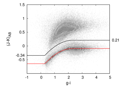
Figure 1: — The colour-colour diagram of VIKING objects with SDSS counterparts. The red line shows the stellar locus, obtained from fitting a quadratic equation in the range [0.3,2.3] to the sample with VSA probability of being a star $>0.95$. The black line is offset +0.3 mag from the locus, representing the adopted star/galaxy separation cut. Objects without SDSS identifications are classified according to their $J-Ks$ colour only, leaving a stripe of $-0.34<(J-{\textit{K}_{s}})_{AB}<0.21$ where the colour-based classification is ambiguous.

3 Applying the Likelihood Ratio method

3.1 The Likelihood Ratio method

One of the earliest approaches (de Ruiter, Arp & Willis, 1977; Prestage & Peacock, 1983; Wolstencroft et al., 1986) to the matching of two source catalogues in different wavelengths uses the ratio of two likelihoods: the likelihood that a true counterpart is observed at a distance $r$ from the source and with magnitude $m$, and the likelihood that an unrelated background object is observed with the same properties:

$$L=\frac{P(r,m,id)}{P(r,m,chance)}$$ (1)

The probability $P(id|r,m)$ that an object at distance $r$ and with magnitude $m$ is a true counterpart, also called the reliability, is then:

$$P(id|r,m)=\frac{L}{L+1}$$ (2)

using Bayes’ theorem and the theorem of total probability.

Sutherland & Saunders (1992) extended the likelihood ratio by incorporating information about other potential counterparts to one source in the calculation of the reliability, and also including additional information (denoted by $c$) which can be, for example, colour information or star/galaxy classification. This is especially useful in a situation where the matching catalogue has a high surface density so that there is a high probability of there being more than one possible counterpart. The reliability $R_{j}$ that the $j$th candidate for one source is the true counterpart is then:

$$R_{j}=P(id|r,m,c)_{j}=\frac{L_{j}}{\sum_{i}L_{i}+(1-Q)}$$ (3)

where $i$ runs over all candidates for this source, and $Q$ is the probability (for a random source) of finding a genuine counterpart above the limiting magnitude of the matching survey. In contrast to equation (2), this includes information about other candidate counterparts to the source. To clarify this distinction, equation 2 is the reliability without information about other candidates for the same source (e.g. picking one candidate at random from a concatenated list of all candidates for a large number of submm sources), while equation 3 is the reliability given the set of all candidate matches for one given source.

Sutherland & Saunders (1992) define $q(m,c)$, the probability distribution of the true counterparts with magnitude $m$ and additional property $c$, and $f(x,y)$ the probability distribution of the source positional errors $x,y$, normalised such that

$$\int\int_{-\infty}^{+\infty}f(x,y)\,dx\,dy=1\hskip 3.61371pt\text{and}\hskip 1.4457pt\int_{-\infty}^{M_{lim}}q(m,c)\,dm\,dc=Q$$ (4)

where $M_{lim}$ is the limiting magnitude in the matching catalogue. It is usually assumed that the positional errors are independent of the magnitude and other additional information, so that $P(m,x,y,c,id)=P(m,c,id)P(x,y,id)$. If $n(m,c)$ is the surface density of unrelated background objects per unit magnitude, the likelihood ratio for any candidate match is then:

$$L=\frac{P(m,c,x,y,id)}{P(m,c,x,y,chance)}=\frac{q(m,c)f(x,y)}{n(m,c)}$$ (5)

In practice, the probabilities above have to be estimated from the data by fitting simple models. The surface density of unrelated background objects is estimated from the surface density of objects in the matching catalogue. The next two subsections explain how we estimate the distributions $f(x,y)$ for the positional errors and $q(m)$ for the true counterparts.

3.2 Positional uncertainties

We here adopt the simple model that the H-ATLAS source positional errors are Gaussian with equal RMS $\sigma_{pos}$ in each of RA and Dec; then the normalisation condition above requires

$$f(x,y)=f(r)=\frac{1}{2\pi\sigma_{pos}^{2}}\exp(-\frac{r^{2}}{2\sigma_{pos}^{2}})\ .$$ (6)

where $r=\sqrt{x^{2}+y^{2}}$ is the radial position difference , and we note $f(r)$ has units of (solid angle)^-1. Smith et al. (2011a) have estimated the positional errors of $>5\sigma$ SPIRE sources, using histograms in RA and Dec of the total number of SDSS sources within a 50” box around the SPIRE 250 $\mu$m centres and taken the clustering of the SDSS objects into account. To be able to use their results, we measure the correlation of our VIKING objects to the SDSS objects, constructing the corresponding RA and Dec histograms, with VIKING objects within a box around the SDSS positions. The 1$\sigma$ VIKING position errors are $<0.2^{\prime\prime}$ and therefore negligible compared to the SPIRE errors. We hence adopt the weighted mean 1$\sigma$ positional uncertainty of $\sigma_{pos}=2.40^{\prime\prime}\pm 0.09$ quoted in Smith et al. (2011a) and assume the errors to be symmetric in RA and Dec.

In theory, the positional uncertainty should depend on the SNR (signal-to-noise ratio) and the FWHM of the observations. Ivison et al. (2007) derive the positional uncertainty as $\sigma=0.6\times\frac{\rm{FWHM}}{\rm{SNR}}$. Following Smith et al. (2011a), we adjust the formula to match our mean positional error by inserting a scaling factor of $1.09$, so that:

$$\sigma_{pos}=0.655\times\frac{\rm{FWHM}}{\rm{SNR}}$$ (7)

with the SPIRE mean FWHM$=18.1^{\prime\prime}$. For each SPIRE source, the positional uncertainty from equation 7 is then used in our LR calculation. We also set a minimum of $\sigma_{pos}=1^{\prime\prime}$ for sources with high SNR, as there are limitations to the minimum positional accuracy from SPIRE and SDSS maps, as discussed in Smith et al. (2011a). We adopt a conservative search radius of $10^{\prime\prime}$ which would include $99.996\%$ of the real counterparts assuming Gaussian errors; in practice, there is evidence for slightly non-Gaussian wings (see Hoyos et al., in prep.), but this radius still includes almost all genuine matches.

3.3 Estimation of $q(m,c)$ and $Q$

We estimate the probability distribution $q(m,c)$ of the true counterparts by using the background subtracted sample of candidate matches, as outlined in Ciliegi et al. (2003). For each class ($c=$ galaxies and $c=$ stars), we estimate $q(m)$ from the data as follows:

• create a magnitude distribution $total(m)$ of all objects within a search radius of 10” around the SPIRE sources

• background subtract $total(m)$ to obtain the so-called $real(m)$ distribution.

• normalise $real(m)$ so that $q(m)=\frac{real(m)}{\sum_{m_{i}}real(m_{i})}\times Q_{0}$

where we sum over bins of magnitude.The background is determined from the number density $n(m)$ measured from the whole catalogue, scaled to a 10” circle. The normalisation factor $Q_{0}$ is an estimate of the probability of finding a counterpart in the VIKING survey down to the $5\sigma$ survey limit, $Q$ in equation (4).

A reasonably accurate value of $Q_{0}$ is important, since this enters the reliability formula above, equation 3. Simply estimating $Q_{0}$ via a stacking analysis (summing $real(m)$ and dividing by the number of SPIRE sources) is not ideal, since source clustering and/or genuine multiple counterparts will tend to overestimate $Q_{0}$ by multi-counting, and therefore reliability estimates will be biased high.

To avoid this multi-counting problem, we decide to estimate $1-Q_{0}$, the fraction of SPIRE sources without a VIKING-detected counterpart, hereafter called blanks: these will be mostly real sources fainter than the VIKING limit, but also including counterparts outside the search radius and spurious SPIRE detections (if any). We start by counting the observed blanks to a given search radius $r$; we then need to correct for those sources that have VIKING candidate matches, where the match(es) are in fact unrelated to the SPIRE source. The number of true blanks is the number of observed blanks, plus the number of true blanks that have been matched with a random VIKING object. To estimate the latter, we create a catalogue of N (=number of SPIRE sources) random positions and cross-match with the VIKING catalogue. Hence, defining $\bar{R}$ as the number of blanks at random positions, $R$ the number of random positions with a VIKING source within 10” and $\bar{S}$ the number of observed SPIRE blanks, we can calculate the number $\bar{S}_{t}$ of true SPIRE blanks as follows:

$$\bar{S}_{t}=\bar{S}+\big{[}\bar{S}_{t}\times\frac{R}{N}\big{]}\Leftrightarrow\bar{S}_{t}=\frac{\bar{S}}{1-R/N}=\frac{\bar{S}}{\bar{R}/N}$$ (8)

Dividing by N provides us then with the fraction of the SPIRE sources that are true blanks, $\bar{S}_{t}/N=\bar{S}/\bar{R}$, which is our estimate for $1-Q_{0}$. Thus, we only need to divide the number of SPIRE blanks by the number of random blanks, for a given search radius.

For our default search radius of 10”, we obtain $1-Q_{0}=0.25$, or $Q_{0}=0.75$. We could use this value in our subsequent LR analysis; however, it depends on the value of the search radius and the $Q$, as defined in equation (4), of the VIKING catalogue is independent of the search radius. We would like to obtain an estimate $Q_{0}$ of $Q$ that is independent of the radius and so repeat the above procedure for radii in the range 1-15”. The values we obtain for the fraction of true blanks are shown in Fig. 2 as black points.

We then model the dependence of the true blanks on the search radius as follows: a SPIRE blank at radius $r$ is a source whose counterpart is either fainter than the VIKING limit, or lies outside the search radius, or both. The former probability is $1-Q_{0}$, this is the first term in equation (9). The probability of the counterpart to reside outside the search radius can be calculated from the positional error distribution $f(r)$, leading to our second term in equation (9). The third term follows if we assume that both possibilities are independent of each other, and using the standard probability result $P(A\ {\rm or}\ B)=P(A)+P(B)-P(A\ {\rm and}\ B)$. Our model for the dependence of the true blanks on the search radius $r$ is then:

$$\begin{split}&(1-Q_{0})+(1-F(r))-(1-Q_{0})(1-F(r))=1-Q_{0}F(r)\hskip 72.26999pt\\ &\text{where}\hskip 7.22743ptF(r)=\int_{0}^{r}P(r^{\prime})dr^{\prime}=1-e^{-\frac{r^{2}}{2\sigma^{2}}}\\ &\text{and}\hskip 7.22743ptP(r)=2\pi rf(r)\end{split}$$ (9)

Fitting this model to the data, we obtain $Q_{0}=0.73\pm 0.03$ as our best-fitting value. Fig. 2 shows the best fit model as the black line and the black filled circles as our data points ($\bar{S}/\bar{R}$ for each radius).

The model underestimates the number of SPIRE blanks in the data in the range $4^{\prime\prime}\leq r\leq 8^{\prime\prime}$ and overestimates the data for $r>10^{\prime\prime}$. This might show some evidence for clustering of the VIKING objects which we have not explicitly considered, but which is accounted for in the value of the mean positional uncertainty $\sigma_{pos}=2.4^{\prime\prime}$ by Smith et al. (2011a); they convolve their model with the clustering signal of the SDSS sources to obtain the value we adopt here. It might also demonstrate that the Gaussian approximation for the SPIRE positional errors, our equation (6), is not entirely accurate. This is also evident when investigating histograms of distances of VIKING and SDSS objects to SPIRE sources. We see slightly higher numbers of objects at distances of around 10” than expected if we assume a Gaussian error distribution. This assumption is examined and will be discussed in Hoyos et al. (in prep.).

Our fitted value of $Q_{0}=0.73$ is consistent with the value of $Q_{0}=0.75$ from the datapoint at our search radius of $10^{\prime\prime}$, and is more conservative. We hence adopt the fitted value $Q_{0}=0.73$ for our subsequent LR analysis.

Having estimated the general value of $Q_{0}$, we still need to know the individual contributions from stars and galaxies, $Q_{0s}$ and $Q_{0g}$ respectively, with $Q_{0}=Q_{0s}+Q_{0g}$. A drawback of the above approach is that we cannot separate our blank SPIRE fields into stars and galaxies. Therefore, we estimate the value of $Q_{0s}$ in applying equation (10) of Smith et al. (2011a), using a background subtracted sample of possible matches within 10”, yielding a value of 0.004. This is very small indeed and shows how unlikely it is that stars are detected with SPIRE. For our LR analysis we then adopt $Q_{0g}=0.72$ and $Q_{0s}=0.01$, the values for $Q_{0}$ used in the normalisation of $q(m)$ for galaxies and stars respectively.

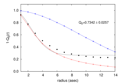
Figure 2: — Illustration of the procedure to estimate $1-Q_{0}$. The red crosses show the fraction of blank SPIRE sources within search radius $r$, while the blue stars show the same fraction for random positions. The black filled circles represent the data points obtained from dividing the number of blank SPIRE positions by the number of blank random positions, our estimate for $(1-Q_{0})F(r)$. The black line represents the best fit to the model $(1-Q_{0})F(r)$, see equation (4), with $Q_{0}=0.7342\pm 0.0257$.

3.4 Probability of mis-identifying a true counterpart

Given the above model, we now estimate $P(wrongID|m_{true})$, defined to be the probability that a true counterpart with a given VIKING ${\textit{K}_{s}}$ magnitude $m_{true}$ is not the best candidate using our LR method. This situation occurs, if the true counterpart has a likelihood ratio value $L=L_{i}$ and there exists a chance match with $L>L_{i}$ for the same source. Hence:

$$\begin{split}P(wrongID|\,m_{true})=&\int_{0}^{L_{max}}P(L_{i}|m_{true})\\ &\times P(chance>L_{i})\,dL_{i}\end{split}$$ (10)

The probability $P(chance>L_{i})$ that there exists a chance match with $LR>L_{i}$ for one SPIRE source can be estimated through simulations. The steps of the procedure we have used are as follows:

• Create $N$ random positions on an area common to both VIKING and H-ATLAS in the G09 field

• For each random position, calculate the likelihood ratio $L$ for random matches, if any, in the VIKING catalogue.

• Create the distribution $D(L)$ of the highest likelihood ratio value for each random position.

From the probability distribution $D(L)$ of the highest LR values for candidate matches to random positions, we can calculate the probability that a given source has a chance candidate above $L_{i}$ by chance:

$$P(chance>L_{i})=\frac{1}{N}\int_{L_{i}}^{L_{max}}D(L)\,dL$$ (11)

A similar method has been employed by Dye et al. (2009) to calculate the probability of radio associations to the BLAST (Balloon-borne Large Aperture Submillimetre Telescope) submm sources. Fig. 3 shows the resulting distribution $D(L)$ from $>10^{6}$ random positions, together with the histogram of the likelihood ratio values of the candidate matches to the real SPIRE positions and of the subset of reliable counterparts (e.g. objects with a probability of $>80\%$ of being the true counterpart, see section 5.1).

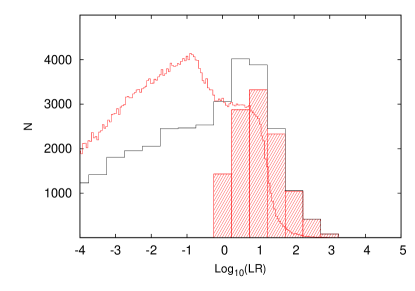
Figure 3: — The solid red line shows the distribution $D(L)$ of the highest $L$ values of candidate matches to $>10^{6}$ random positions in the G09 field. The peaks at lower and higher $L$ values are due to star and galaxy matches respectively. The black histogram represents the LR values of all candidate matches to the SPIRE positions. The filled red histogram represents the reliable matches only.

The probability $P(L_{i}|m_{true})$, the first factor in the integral in equation (10), that a true counterpart with ${\textit{K}_{s}}$ magnitude $m_{true}$ acquires the likelihood ratio $L_{i}$ can be calculated analytically from the probability distribution $P_{r}(r)=2\pi rf(r)$ of the offsets. For a given $m=m_{true}$ we have $f_{i}=f(r)=L_{i}\times n(m_{true})/q(m_{true})$ and hence $P(L_{i}|m_{true})=P_{f}(f_{i})$. We can find the probability distribution $P_{f}(f)$ from $P_{r}(r)$ by performing a variable transformation:

$$P_{f}(f)=-P_{r}(r(f))\times\frac{dr}{df}=2\pi\sigma^{2}$$ (12)

This is a surprisingly simple result, i.e. for Gaussian errors, $P_{f}(f)$ has a uniform distribution between 0 and its maximum value $1/2\pi\sigma^{2}$. We would like to note though that the positional uncertainty depends on the value of the SNR. For simplicity, we have used the value of $\sigma_{pos}=2.4^{\prime\prime}$, allowing for most of the SPIRE sources to have a SNR value close to 5. A more detailed analysis could take into account the probability distribution of the SNR values of all SPIRE sources.

Having calculated the probability of a true counterpart with assumed magnitude $m_{true}$ not being the best candidate in our LR method, we can then calculate $P(wrongID)$, the same probability integrated over the model magnitude distribution of the true counterparts:

$$P(wrongID)=\frac{\int_{0}^{M_{lim}}P(wrongID|m)\,q(m)\,dm}{\int_{0}^{M_{lim}}q(m)\,dm}$$ (13)

Using the distribution $D(L)$ from the random positions, our VIKING sample as described in section 2.2 to derive the magnitude distributions $q(m)$ and $n(m)$, as well as $\sigma_{pos}=2.4^{\prime\prime}$, we obtain $P(wrongID)=0.0493$. We hence expect to mis-identify around $\sim 5\%$ of the true VIKING counterparts to the SPIRE sources.

This is likely to overestimate the true value because we have not taken the individual SNR values of the SPIRE sources into account. This performance measure of the LR method is compared in section 5.1 with the false identification rate for reliable counterparts.

4 Photometric redshifts

The submm wavebands benefit from negative k-correction with the effect that objects can be detected at least out to $z\gtrsim 5$ in the $870\,\mu{\rm m}$ band (Blain & Longair, 1993; Chapin et al., 2011). Selecting sources at $250\,\mu{\rm m}$ reduces the effectiveness of the negative k-correction, but models still predict a significant fraction of the SPIRE sources to reside at $z>1$ (e.g. Amblard et al., 2010; Lapi et al., 2011).

A significant fraction of our VIKING counterparts ($\sim 28\%$) have spectroscopic redshift from the GAMA and SDSS redshift surveys. For the remainder, we will obtain photometric redshifts by combining the near-infrared photometry with optical photometric information from the SDSS survey. Objects with spectroscopic redshift from the GAMA survey are then employed as a training set to estimate the photometric redshifts using neural networks, see below.

SDSS matches are found for $\sim 68\%$ of the VIKING candidates within $2^{\prime\prime}$ by performing a simple nearest neighbour match. The remainder of the VIKING objects are too faint to be detected in the SDSS survey. For near-complete visible detections we have to wait for the VST KIDS survey, which will observe the VIKING areas down to 24.8, 25.4, 25.2 and 24.2 (10$\sigma$, AB) in ${u^{\prime},g^{\prime},r^{\prime},i^{\prime}}$ bands respectively, thus giving detections in at least $r^{\prime},i^{\prime}$ bands for nearly all VIKING objects.

With a search radius of $2^{\prime\prime}$ we are unlikely to identify a wrong SDSS counterpart. Using the surface density of the SDSS catalogue employed for the optical matching by Smith et al. (2011a), we estimate around 2% (170 objects) of our subsample of reliable VIKING matches to have a wrong SDSS identification within $2^{\prime\prime}$.

For photometric redshifts, we use a neural network method in which the photometry of objects with available spectroscopic redshifts provides the sample to train a network. Once trained, the network is then used to obtain photometric redshifts from the photometry of objects without reliable redshift information. The photometry in the different bands employed can differ, for instance we are using SDSS modelmags and VIKING Vega aperture magnitudes. In contrast, a template fitting method where the photometry is compared to the expected photometry from a class of different (empirical and/or theoretical) SEDs (Spectral Energy Distribution), needs to use very carefully calibrated photometry in all bands. The software used to obtain the photometric redshifts is ANNz (Collister & Lahav, 2004), a publicly available product. We train a committee of 3 networks for each possible photometric band combination, recommended to minimise the network variance. The output of ANNz is the photometric redshift for each object together with a redshift error estimate which takes the photometric errors in each band into account.

We use 30,697 objects with photometry from SDSS and VIKING and spectroscopic redshifts from GAMA in our training set. The median spectroscopic redshift of the GAMA sample is $\tilde{z}_{spec}=0.211$. The median redshift of the VIKING counterparts is expected to be higher and the training set should reflect this. Currently, there are no deeper spectroscopic surveys available that overlap with the VIKING area. There are though some deeper spectroscopic redshifts from surveys that are within the UKIDSS LAS area (Lawrence et al., 2010; Hewitt et al., 2006). Therefore, we undertake a comparison of WFCAM and VISTA photometry, to be able to use deeper photometric information from the zCOSMOS (Lilly et al., 2007) and DEEP2 (Davis et al., 2003) surveys. We match VIKING objects in a 4 deg² area in the H-ATLAS SDP field to objects in the UKIDSS LAS and obtain the mean and standard error for the difference in magnitudes (apermag3) in each of the bands YJHK. We are then able to use the LAS photometry for these samples by subtracting this mean from the LAS magnitudes and adding the standard error of the difference in quadrature to the photometric error. This allows us to use the deeper photometry and spectroscopic redshifts of zCosmos (1530 objects) and DEEP2 (238 objects), which overlap with the UKIDSS LAS survey (but not with VIKING), as a training set.

Adding all our subsamples together, we obtain an overall training catalogue with 32,465 spectroscopic redshifts. We then compile a photometric catalogue for all VIKING candidate matches with ugriz photometry (modelmags) and YJHK photometry (aperture magnitudes), where present. We attempt photometric redshifts where we have at least 2 infrared bands with good photometry.

Using the deeper spectroscopic redshifts from zCOSMOS and DEEP2 forces us to exclude the VIKING Z band in the training catalogue. Investigating how this influences our photometric redshifts, we create a second training catalogue, this time using just the GAMA subset (95% of the first training catalogue), so that we can include the VIKING Z band. The scatter in the differences between photometric and spectroscopic redshifts for objects with a spectroscopic redshift is slightly lower for this second training set, but this is to be expected because we compare only the lower redshift end. Assuming that the inclusion of deeper redshifts into the training set reflects the true VIKING redshift distribution better, we adopt the photometric redshifts from our first training catalogue, the GAMA-zCOSMOS-DEEP2 training set.

5 Results

5.1 ${\textit{K}_{s}}$ band matching

There are 22,000 SPIRE sources within the sky area corresponding to the G09 VIKING object catalogue. Of those, 18,989 sources have at least one possible match within a search radius of $10^{\prime\prime}$ in the VIKING ${\textit{K}_{s}}$ band selected catalogue, with a total of 35,800 candidate matches; of which 30,659 are classified as galaxies (85.6%) and 5,141 are classified as stars (14.4%), as described in section 2.3. Table 1 shows the number of SPIRE sources matched as a function of the number of candidate matches found per position.

There are 11,294 SPIRE sources with a best VIKING counterpart with a reliability $>80\%$ (11,282 galaxies/12 stars). This means we were able to match $\sim 51\%$ of the SPIRE sources with a high reliability. We will refer to the set of matches with $R>0.8$ as “reliable” hereafter (as we show later, the mean reliability of this set is near 0.96). Fig. 4 shows the magnitude dependent distribution $q(m)/n(m)$ for galaxies and stars used in the calculation of the LR values. Fig. 5 and  6 show the magnitude distributions involved in estimating $q(m)$: of the background $n(m)$, of the possible matches $total(m)$ and of the background subtracted sample $real(m)$. Also shown in the figures is the magnitude distribution for reliable counterparts. The reliable matches show a lower fraction of fainter counterparts compared to all candidate matches, representing the steep increase of fainter objects in the background number counts, causing lower reliability values for fainter matches.

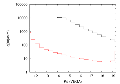
Figure 4: — The magnitude dependent part $q(m)/n(m)$ of the LR analysis, calculated from the data as described in section 3.3. The black line indicates the galaxy candidates, the red line shows the stellar candidates. The values for the bright bins for the galaxy distribution were extrapolated from the first bin that included more than 10 galaxies, at $m=13.4$.

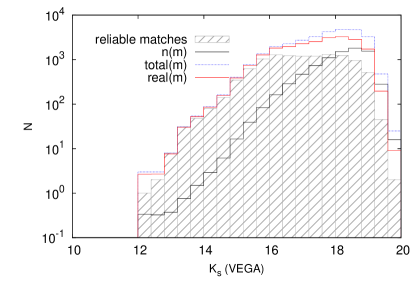
Figure 5: — The magnitude distributions involved in estimating $q(m)$ for galaxies. Here $n(m)$ (solid black) is the distribution of the background objects, calculated from the whole VIKING G09 catalogue, as described in section 2.3, and $total(m)$ (dashed blue) is the magnitude distribution of all possible matches within $10^{\prime\prime}$. $real(m)$ (solid red) is the background subtracted distribution as described in section  3.3 and is significantly brighter than the background. The light grey shaded histogram represents the magnitude distribution of the reliable matches.

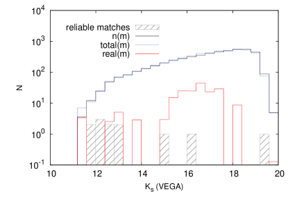
Figure 6: — The magnitude distributions involved in estimating $q(m)$ for stars. The colour scheme is as in Fig. 5.

We can estimate a false ID rate by summing up the complement of reliability values of the reliable matches:

$$N_{falseID}=\sum_{i}(1-R_{i})=469.25$$ (14)

corresponding to a mean reliability of $0.958$ and a false ID rate of $4.2\%$.

In the appendix, we show cut-outs of VIKING and SDSS images around SPIRE sources for 9 positions drawn at random from our reliable sample.

Table 1: The distribution of the number of VIKING ${\textit{K}_{s}}$ band sources within 10” of the 250 $\mu m$ SPIRE positions. Of the 22,000 sources in the VIKING area, 8118 have only one possible match within 10” and $59.7\%$ of these are determined to be reliable. This emphasises the difference from a simple nearest neighbour match.

N(matches)	N(SPIRE)	N(reliable)	%
0	3011
1	8118	4851	59.76
2	6619	4040	61.04
3	2968	1710	57.61
4	968	529	54.65
5	241	128	53.11
6	63	31	49.21
7	11	5	45.45
8	1	0	00.00
Totals	22,000	11,294

5.2 VIKING and SPIRE colours

Fig. 7 shows the ZJK colour-colour diagram of the 10,121 reliable counterparts (red) with 5$\sigma$ detection in all 3 VIKING bands. Colours from randomly selected background galaxies are depicted in grey. The redshift evolution of the submm selected mean galaxy template of Smith et al. (2011b) is shown in green. The template has been artificially redshifted between $z=0-1.5$ in intervals of $dz=0.1$ and colours have been computed by integrating the product of the template SED with the VISTA response functions at each redshift interval. A small deviation from the Vega system is present in the VISTA $Z$-band and a measured offset (Findlay et al., 2012) has been added to the colours computed here to reflect this.

The median $Z-J$ and $J-{\textit{K}_{s}}$ colours for the reliable matches are $0.97$ and $1.64$; for the background objects the median colours are $0.89$ and $1.54$. Performing a two-sided K-S test on the $J-{\textit{K}_{s}}$ and the $Z-J$ colours for reliable matches and the background objects enables us to reject at a significance of 99.96% that the two populations are drawn from the same distribution for either colour. Thus, we find evidence that the reliable matches to the SPIRE sources are slightly, but significantly redder than the population of all VIKING objects in the G09 field.

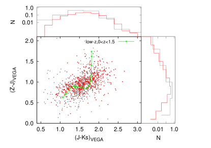
Figure 7: — VIKING colour-colour diagram of reliable counterparts (red) and background galaxies (grey) with 5$\sigma$ detections in $Z$,$J$ and ${\textit{K}_{s}}$. The horizontal and vertical histograms show the distributions in $J-{\textit{K}_{s}}$ and $Z-J$ respectively. The green points connected by a green line represent the evolutionary track of a typical H-ATLAS galaxy SED for $z<0.35$ from Smith et al. (2011b) and calculated by (Findlay et al., 2012).

Within the search radius of $10^{\prime\prime}$, 3011 sources have no 5$\sigma$ ${\textit{K}_{s}}$ VIKING candidate, i.e. they are almost certainly fainter than the VIKING limit. Fig. 8 shows $S_{250}/S_{350}$ histograms separately for the sources with a reliable match (best $R>0.8$), sources with non-reliable match(es) (best $R<0.8$), and for sources that are blank in VIKING (black, red and shaded red respectively). The blank sources (median=1.01) have distinctively redder colours than the sources with reliable matches (median=1.32), suggesting that they reside at higher redshifts with the peak of the dust emission moving to longer wavelengths. The colours of sources with unreliable matches (median=1.11) lie in between the other two populations, indicating that they might be composed from members of both populations.

From our value of $Q_{0}$, we expect around 60% of the unreliably matched sources to have a true counterpart, but for which we do not have a high enough reliability, with the remaining 40% being matched to unrelated background objects. Smith et al. (2011a) find a similar trend in the distribution of the $S_{250}/S_{350}$ colour of SPIRE sources in the SDP field matched to the SDSS $r$-band catalogue for the 3 different populations.

We also show a SPIRE colour-colour diagram of the sources in Fig. 9. The colours of the reliably matched and the blank sources are very similar to those in Smith et al. (2011a), their fig. 9. This figure can also be compared to fig. 1 in Amblard et al. (2010). We add the evolutionary tracks of two templates: a low-z template compiled by Smith et al. (2011b) from optical counterparts to SPIRE sources out to $z\simeq 0.35$ (blue line) and the submm template from Lapi et al. (2011) (green line), thought to be appropriate for high-z H-ATLAS sources at $z>1.2$. From the tracks of the two SED templates we can again suggest that the blank sources lie at higher redshifts in general than the sources with reliable matches. Assuming that the H-ATLAS sources are comprised of two distinct populations, see section 5.5, a lower redshift population with mainly normal galaxies (with a much higher star-formation rate than local normal galaxies), and a higher redshift population of dusty submm galaxies (likely to be giant proto-spheroidal galaxies in the process of forming most of their stars), our blank sources could represent a mixture of the former at $z\gtrsim 0.7$ and the latter at $z\gtrsim 1.5$.

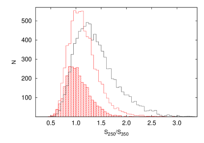
Figure 8: — Distribution of the SPIRE $S_{250}/S_{350}$ colour. Black: sources with reliable matches. Red: sources that have unreliable matches only. Red shaded: blank sources. The blank sources show distinctively redder colours than the other two populations, suggesting they are at higher redshifts.

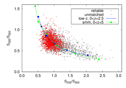
Figure 9: — Colour-colour diagram of SPIRE objects with $5\sigma$ detection in $250\mu m$ and $350\mu m$ and $3\sigma$ detection in $500\mu m$. The dark grey points represent SPIRE sources that have reliable counterparts, the red points show the colours of blank SPIRE sources. The blue points connected by the blue line represent the colours of a typical H-ATLAS galaxy SED for $z<0.35$ from Smith et al. (2011b). The dots are at an interval of $z=0.5$, starting at $z=0$ on the right hand side. The green points connected by the green line represent the colours of the submm SED in Lapi et al. (2011). The points are at an interval of $z=1$, starting with $z=0$ on the right.

5.3 Multiple counterparts

The LR method assumes that there is only one true counterpart to each source, and assigns reliabilities self-consistently based on this, so that the sum of reliabilities cannot exceed 1. Thus, if more than one counterpart with $R>0.2$ is present, we will not find a reliable match. If individual reliabilities add up to our threshold of $0.8$, we could assume that these candidate matches are all associated with the sources, either through confusion or in a real physical sense (i.e. merging galaxies).

In our results, we find 1444 SPIRE sources that fulfill the above criteria and potentially have multiple true counterparts in VIKING. Most of those will have additional close chance objects within the search radius, denying a reliable identification, but some might be genuine mergers or constitute members of the same cluster. We can rule out a chance match by comparing the redshifts of all possible matches to one SPIRE source. Checking for available redshifts in the GAMA and SDSS spectroscopic redshift databases, we find matches to 37 sources whose redshifts are within 5$\%$ of each other. The mean redshift difference is 0.0011 with a maximum difference of $\bigtriangleup z=0.0187$. Those could be either merging galaxies or members of the same cluster.

We use our photometric redshifts, see section 5.5, to select further candidates. We account for the higher errors in the photometric redshifts by allowing a redshift difference of 10$\%$ and also compare photometric redshifts of possible matches for which we do not have a spectroscopic redshift with spectroscopic redshifts of other candidates to the same source. We find 602 further sources where the SPIRE flux potentially originates from an interacting system or from galaxies within the same cluster. Fig. 10 shows a VIKING ${\textit{K}_{s}}$ image cutout around one of the those sources, HATLAS J091017.1-005538. Due to the uncertainties in the photometric redshifts, those sources can only be regarded as candidates and need further investigation to be confirmed as interacting systems or as members of the same cluster.

It would be interesting to confirm how many sources definitely do not have physically related multiple counterparts and are just unreliable matches, but this is difficult due to the sparsity of available spectroscopic redshifts and the uncertainties on the photometric redshifts. However, we can estimate the number of reliable identifications we are missing due to potentially multiple counterparts. From Table 1, we can see that the identification rate for reliable counterparts is approximately 60$\%$ without the presence of additional potential matches. We do not see a decrease in the identification rate for sources with two possible matches, suggesting that the true number of merging galaxy pairs is indeed low. For sources with higher numbers of possible matches, we have an increased possibility of having observed a galaxy cluster and so the identification rate for reliable matches falls. For instance, sources with 4 possible matches have an identification rate of around 55%, suggesting that we miss 5% of the reliable matches, equivalent to 50 sources. Adding up the missed reliable matches of all sources with more than 2 possible counterparts, suggests that we are missing around 150 reliable VIKING counterparts due to additional matches within our search radius. This is a small number indeed, only around $10\%$ of the number on our list of candidates for true multiple counterparts. There is evidence, from observation and simulation, for the merger rate to evolve with redshift and to peak at $z\simeq 1.2$ (Bell et al., 2006; Lotz, 2007; Ryan et al., 2008), beyond the redshift of most of our reliable counterparts. Hence, we might miss a substantial fraction of mergers not because we find multiple candidates but rather because they hide in the fraction of blank SPIRE sources. This implies that our candidate list comprises mostly either chance alignments of galaxies or cores of clusters of galaxies resulting in confusion when observed with SPIRE.

Figure 10: — VIKING ${\textit{K}_{s}}$ image of HATLAS J091017.1-005538, 12” on the side. The black cross indicates the SPIRE position and the black circle represents the 2$\sigma=2.9^{\prime\prime}$ positional uncertainty of this SPIRE source. The blue circled object has reliability $R=0.74$, the red circled object has $R=0.25$. The third candidate has negligible reliability, but could still be part of the interacting system.

5.4 Stellar matches

The far-infrared/submm mainly detects cold, dusty objects. It is unlikely that stars are detected with SPIRE, unless they are post-AGB, shrouded in dust or have debris disks (e.g. Thompson et al., 2010). We have matched 12 SPIRE sources reliably to point-like objects. Their location on the $J-{\textit{K}_{s}}$ vs $g-i$ colour-colour diagram is displayed in Fig. 11.

HATLAS J090450.4-014525 (884 in Fig. 11) displays galaxy-like colours and is listed as a QSO in the quasar catalogue of Véron-Cetty & Véron (2010). All other objects are consistent with having star-like colours.

Two blazars were identified by Gonzáles-Nuevo et al. (2010) in the SDP field from cross-matching to radio observations. We match H-ATLAS J090910.1+012135 reliably to a point-like VIKING object (sgmode$=10$, i.e. point-like object classified as a galaxy on the basis of a non-stellar spectroscopic redshift). H-ATLAS J090940.3+020000 is not matched reliably within our search radius of 10”. We find one possible VIKING counterpart within 10” of this SPIRE source: a bright point-like object (${\textit{K}_{s}}=15.03$, sgmode$=10$), lying at a distance of nearly 9” from the SPIRE position and therefore obtaining a low reliability. However, it lies within 1” of the known blazar PKS 0907 +022, the object identified as the blazar counterpart to H-ATLAS J090940.3+020000 by Gonzáles-Nuevo et al. (2010). Despite the low reliability, there is hence evidence that our VIKING object is the counterpart to H-ATLAS J090940.3+020000. The colours of both VIKING objects are shown in Fig. 11 as blue dots. Blazars in the H-ATLAS Phase 1 fields are currently investigated by a team led by Marcos Lopez-Caniego with 14 candidates identified so far.

For the brighter stars, it is a possibility that the measured SPIRE flux originates from a galaxy that is too faint in the near-infrared to be detected by VIKING, or obliterated by the star, and the star is a chance projection. The reliabilities of star counterparts are on average lower ($\bar{R}=0.85$) than for the reliable galaxy matches, due to the lower $Q_{0}$ value and the lower values of $q(m)$ (see Fig. 4).

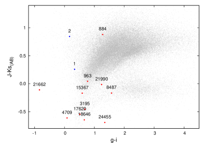
Figure 11: — Reliable stellar matches, represented by the red dots. For clarity we have labeled the dots with row numbers from the SPIRE catalogue and not with the full HATLAS names. HATLAS J090450.5-014525 (884) has galaxy-like colours and was originally selected to be a QSO target of the Sloan spectroscopic survey but has subsequently been rejected as a target. It is listed as a QSO in the Quasar and Active Galactic Nuclei catalogue by Véron-Cetty & Véron (2010) with redshift $z=1.005$. The colours of the other objects are consistent with being star-like. The extreme $J-{\textit{K}_{s}}=-2.67$ value of HATLAS J091233.9-004549 is not shown in the diagram and could be due to saturation. The blue dots represent the colours of the VIKING counterparts to the two blazars found in the SDP field, $1=$H-ATLAS J090910.1+012135, $2=$H-ATLAS J090940.3+020000

5.5 Photometric redshift distribution

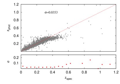
Figure 12: — Upper panel: photometric vs. spectroscopic redshift for 3147 reliable VIKING counterparts with spectroscopic redshift from either GAMA or SDSS. Lower panel: scatter of the difference $|z_{spec}-z_{phot}|$ for the same 3147 objects in redshift bins of $\delta z=0.05$.

We have measured the photometric redshifts for all of our 11,294 reliable VIKING counterparts, 8750 of which have SDSS matches within 2”, as described in section 4. Spectroscopic redshifts exist for 3147 of the reliable VIKING counterparts which allows us to evaluate the accuracy of the photometric redshifts, see Fig. 12. The spectroscopic redshifts are taken from either the GAMA or the SDSS redshift survey. Where a redshift exists in both surveys for a VIKING object, we have used the GAMA redshift (quality flag $Q\geq 3$ only). Excluding 31 confirmed QSOs with $z>1$, the scatter of the difference between our photometric redshifts and the spectroscopic redshifts is $\sigma=0.0353$. This reduces to $\sigma=0.0259$ for the normalised redshift distribution $\bigtriangleup z/(1+z_{spec})$.

Also visible from Fig. 12 is the tendency for the photometric redshift to underestimate the redshift at higher values of $z$; for $z>0.3$, the bias amounts to $-0.0889$. The systematic underestimation is also found when comparing spectroscopic redshifts with the photometric redshifts from the H-ATLAS Phase 1 catalogue which used optical and near-infrared photometry from SDSS and UKIDSS-LAS, see Smith et al. (2011a). They have employed a similar training set which suggest that we face an issue with the representativeness of our training set. The reason for the bias seems less likely to be a lack of spectroscopic redshifts at $z>0.3$ but could rather be related to a difference in the colour distribution of galaxies in the training set and our VIKING galaxies. Clearly, more work is needed to investigate the reasons for the bias at $z>0.3$ and, crucially, to assemble a more representative training set which is outside the scope of this paper.

The redshift differences $z_{phot}-z_{spec}$ of the 31 confirmed QSOs with $z>1$ are considerably worse, as the training set includes few high-z QSOs and also the near power-law spectra of QSOs means that QSO photo-z estimates are much worse than for galaxies.

Currently, we cannot estimate the accuracy of the photo-z of VIKING counterparts with just near-infrared photometry due to the lack of spectroscopic redshifts. In general, they have higher photo-z, as can be seen from Fig. 13.

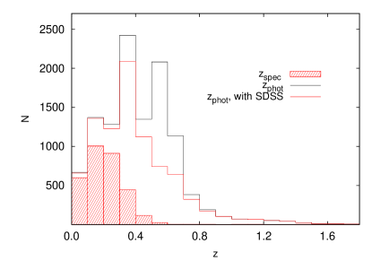
Figure 13: — Redshift distributions for the reliable VIKING matches. The filled boxes represent the spectroscopic redshifts for 3147 of the 11,294 reliable VIKING matches with either GAMA or SDSS spectroscopic redshift with a median redshift of $\tilde{z}=0.199$. The excess peak of all photo-z at $z\sim 0.5$ (black histogram) is formed of redshifts to VIKING objects without optical photometry.

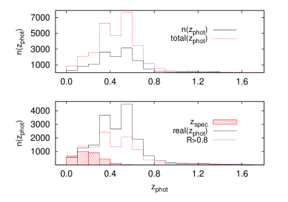
Figure 14: — Upper panel: the dashed red histogram shows the photometric redshift distribution of VIKING background objects, the black line represents the photometric redshift distribution of all VIKING objects within our search radius ($total(z_{phot})$). Lower panel: the expected photometric redshift distribution of the true VIKING counterparts ($real(z_{phot}$, black line), calculated by subtracting the background from $total(z_{phot}$. The filled histogram represents spectroscopic reshifts and the red dashed histogram is the distribution for our reliable counterparts.

Certainly, we are missing more reliable identifications at the higher redshift end than at lower redshifts. The lower panel in Fig. 14 shows a comparison of the expected redshift distribution, $real(z_{phot})$ of the VIKING counterparts to the redshift distribution of our reliable counterparts ($R>0.8$). The expected distribution $real(z_{phot})$ can be calculated in a similar way as the magnitude distributions: from the $total(z_{phot})$, the photometric redshift distribution of the VIKING objects within our search radius of $10^{\prime\prime}$ and the background distribution $n(z_{phot})$, both shown in the upper panel of Fig. 14. Table 2 shows the fraction of reliable to expected counterparts per redshift bin, i.e. the completeness of our photometric redshift sample.

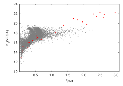
Figure 15: — ${\textit{K}_{s}}$ magnitudes (Vega) versus photometric redshift. Grey dots: our reliable VIKING counterparts. Red points: BLAST sources of Dunlop et al. (2010). This suggests that we are fairly complete out to $z\sim 1$.

Dunlop et al. (2010) have calculated very accurate photometric redshifts for counterparts to 20 bright BLAST sources, using a wide range of deep multi-wavelength data in the GOODS-North field. BLAST used a proto-type SPIRE camera and the BLAST sources were selected down to $36\rm{mJy}$ in 250 $\,\mu{\rm m}$. We compare our reliable sample to their data on a ${\textit{K}_{s}}$ vs $z_{phot}$ in Fig. 15. This plot suggests that we are fairly complete out to redshift $z\sim 1$ and are missing higher redshift counterparts due to the VIKING survey limit.

Table 2: Photometric redshift completeness, calculated from a background subtracted sample of possible counterparts, $real(z_{phot})$. The errors assume that Poisson errors in the $real$ distribution are dominant.

$z_{phot}$	Completeness($\%$)	$\sigma_{comp}$
0.0-0.1	117.8	5.8
0.1-0.2	108.6	3.8
0.2-0.3	87	2.9
0.3-0.4	65.9	1.4
0.4-0.5	50.6	1.3
0.5-0.6	46.3	0.9
0.6-0.7	59.3	1.8
0.7-0.8	56.1	2.7
0.8-0.9	55.8	3.6
0.9-1.0	61	5.6
1.0-1.1	55	5.6

Work carried out by Amblard et al. (2010) using SPIRE and PACS colours, suggests that the SPIRE source redshift distribution might be bimodal, formed by a low redshift population of spirals and a high redshift population of starburst galaxies peaking at $z\sim 2$. Dariush et al. (2011) found that most of the H-ATLAS low-z galaxies are comprised of blue/star-forming galaxies with some highly dusty, red spirals. Evidence for this bimodality in the redshift distribution can also be found in Maddox et al. (2010) using the angular correlation function of 250, 350 and 500 $\mu m$ selected SPIRE sources, and from theoretical models (Lagache et al., 2003; Negrello et al., 2007). Smith et al. (2011a) discuss this in more detail in their section 3.3 on the photometric redshift distribution.

In this work, we find that the large majority of our candidate identifications have $z_{phot}<1$, as expected from the ${\textit{K}_{s}}$ magnitude limit of the VIKING data. From our value of $Q_{0}$, we expect about 27% of the SPIRE sources to be too faint to be detected in VIKING and hence very likely to be at higher redshifts, see section 5.2. Taking into account the possible underestimation of our photometric redshifts at $z>0.3$, we find that $\sim 2\%$ of the H-ATLAS 250 $\,\mu{\rm m}$ sources with a reliable counterpart lie at $z>1$. At least a similar fraction of sources without a reliable match and expected to have a true counterpart in VIKING, should obtain $z>1$. We hence expect $\gtrsim 30\%$ of our H-ATLAS sources to be found at $z>1$. We compare this with the redshift distributions found for BLAST sources and for sources detected by SPIRE in the GOODS-North field.

Dunlop et al. (2010) and Chapin et al. (2011), using 250 $\,\mu{\rm m}$ BLAST sources, both find that $\sim 50\%$ of their sources lie at $z>1$ from a variety of photometric redshifts, even though the shapes of the distributions differ, with Dunlop et al. (2010) seeing a more pronounced bi-modality and Chapin et al. (2011) a greater tail beyond $z=2$. This comprises a significantly higher fraction of high redshift sources than in this work. Dye et al. (2009) find $\sim 30\%$ of their BLAST sources within a deep field to be at $z>1$, fully consistent with our fraction. Having used different selection criteria for their BLAST sources, either signal-to-noise cut-offs or flux limits in any of the 250, 350 or 500 $\,\mu{\rm m}$ BLAST bands, leads to different sub-samples that are difficult to compare. In addition, the methods to obtain photometric redshifts and to identify optical/mid-infrared counterparts vary. It is difficult to disentangle the different approaches, but there is still very broad agreement in the conclusion that we see two different populations, one which, at lower redshifts, we find in VIKING counterparts, and the other, at higher redshifts, the fraction of which we can imply and which is consistent with at least some of the BLAST findings.

A similar picture emerges from the HerMES project (Oliver et al., 2010) so far. Eales et al. (2010) and Elbaz et al. (2010) use deep imaging in small areas ($<0.1\,{\rm deg}^{2}$) observed by SPIRE and with excellent multi-wavelength data available, as well as spectroscopic and photometric redshifts. Both groups use a 250 $\,\mu{\rm m}$ selected sample and assume a 24 $\,\mu{\rm m}$ detection. With a high fraction of spectroscopic redshifts ($>65\%$), Elbaz et al. (2010) find $35-40\%$ of their sources lie at $z>1$ (deduced from their fig. 2), consistent with our findings, whereas Eales et al. (2010) discover close to $50\%$ in this redshift range.

5.6 Towards more complete identifications

So far we have estimated that 73% of SPIRE sources have counterparts in VIKING, while 51% have a reliable match; thus, the reliable sample comprises approx 51/73 = 70 percent of all SPIRE galaxies with both $f_{250}>32\,{\rm mJy}$ and ${\textit{K}_{s}}<19.2$. Of the remaining 49% of SPIRE sources, 14% are undetected in VIKING and 35% have one or more low-reliability match(es); overall we expect around half of these to be genuine matches. To make this decisive, we would need follow-up observations such as radio or ALMA (Atacama Large Millimeter/submillimetre Array, Wotten & Thompson, 2009) imaging giving a sub-arcsec position, or possibly optical/NIR spectroscopy of VIKING candidates (if we can identify SPIRE sources via unusually strong emission lines). This would normally be “decisive” in that a sub-arcsec radio/submm position would either match a VIKING galaxy to very high reliability, or if not it would prove the source is fainter than the VIKING limit.

For non-reliable matches, the total reliability $\sum R_{i}$ for a given source is a good estimate of the probability that the SPIRE source has a real counterpart in VIKING, i.e. the probability that a follow-up will actually find a good match; therefore in a follow-up search we should target the non-reliable matches in descending order of total probability.

Assuming a lower limit of the total probability of 50% (70%) would result in an additional 2380 (1856) identifications for 2967 (2101) observing targets. We would then obtain a sample which is 85% (82%) complete to $f_{250}>32\,{\rm mJy}$ and ${\textit{K}_{s}}<19.2$. If we would use all non-reliable positions as targets, regardless of the total reliability, we would only be able to reach a completeness of 89%. This effect can also be seen in Smith et al. (2011a) where the sum of the reliabilities to all possible counterparts would result in a 44% identification rate, lower than expected from their value of $Q_{0}=0.59$. This shows that our (and their) reliabilities might be underestimated; this is more evidence for a likely non-Gaussian positional error distribution which will be addressed in future publications of the catalogue.

Of additional consideration is our candidate list for multiple identifications, see section 5.3. They display a total reliability of 80% by definition and would hence be included in a possible target list. It would be interesting to see how many of those could be confirmed as true multiple identifications.

Fig. 16 shows the distribution of the total reliabilities for the non-reliable SPIRE positions together with the number of additional identifications we would expect if we followed up all SPIRE positions down to 50 or 70 percent.

It is also useful to compare to the results of Dunlop et al. (2010); as described above, they identified a much smaller sample of 20 BLAST $250\,\mu{\rm m}$ sources, but benefiting from the very deep multiwavelength data in GOODS-S. In their sample, all candidate identifications with $z<1.2$ are brighter than ${\textit{K}_{s}}<19.6$, while all at $z>1.2$ are fainter; this suggests that the 3011 sources without a VIKING counterpart have a high probability of being at $z>1.2$ , and the same applies for the 3194 sources with low-reliability matches $\sum R<0.2$.

Since the flux ratio $f_{870}/f_{250}$ strongly increases with redshift for typical SMGs, the non-identified sources are therefore good targets for ALMA $870\,\mu{\rm m}$ follow-up snapshots; this could give a relatively efficient method for selecting luminous high-z SMGs.

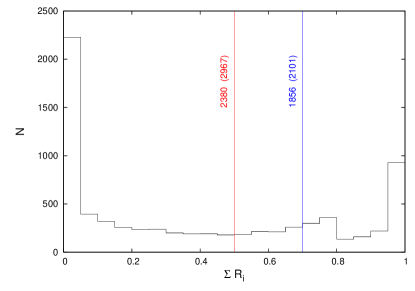
Figure 16: — Total reliability distribution of the non-reliable SPIRE sources. For the 7391 sources without a reliable counterpart, we sum the reliabilities of all possible VIKING counterparts per source. This total reliability is an estimate of the probability that the SPIRE source has a real counterpart in VIKING. If we include all SPIRE positions with total reliabilities greater than 50% for a follow-up, we will have to observe 2967 positions and expect to gain 2380 additional reliable VIKING counterparts (red line and text). The blue line and text show the equivalent for a 70% total reliability.

6 Comparison to optical identifications

6.1 Reliable counterparts

In this section we compare our results with the optical identifications supplied with the H-ATLAS G09 Phase 1 source catalogue. This used a similar likelihood ratio method with an $r$-band selected sample down to $r=22.4$, as explained for the SDP data in Smith et al. (2011a). The VIKING ${\textit{K}_{s}}$-band should be better placed than the optical $r$-band in identifying counterparts to the SPIRE sources. As discussed in the introduction, at higher redshifts ($z\geq 0.5$), the ${\textit{K}_{s}}$ band is detecting flux from the near-infrared restframe, while the $r$ band is restframe blue/UV; thus ${\textit{K}_{s}}$ is much better able to detect dusty galaxies. We therefore expect a higher number of reliable identifications from matching with VIKING than with SDSS. To be able to compare our results, we cross-match our VIKING candidate matches with the SDSS database (DR7) within 2” and choose the nearest (primary) object.

Table 3: — Comparison of the reliable counterparts to the SPIRE sources using optical r-band and near-infrared Ks-band matching. In the area corresponding to the VIKING preliminary source catalogue, we match reliably 51.3% of all SPIRE sources. This is a significant increase in the identification rate compared to the 39.0% of sources that are matched reliably to a SDSS object.

				N(reliable)	with SDSS	N(reliable) not reliable in
band	N(SPIRE)	N(matches)	N(reliable)	in VIKING area	in VIKING area	${\textit{K}_{s}}$	r
${\textit{K}_{s}}$	22,000	35,800	11,294 (51.3%)	11,294 (51.3%)	8,750	-	3,732
r	26,369	36,839	9,623 (36.5%)	8,587 (39.0%)	8,587	1,024	-

We concentrate on the reliable counterparts of both surveys. The Phase 1 catalogue lists 9623 reliable optical counterparts ($36.5\%$) to 26,369 5$\sigma$ SPIRE sources in the G09 field; of the reliable counterparts, there are 8587 ($39.0\%$) in the VIKING observed area. In comparison, we are able to match 11,294 SPIRE sources ($51.3\%$) reliably to VIKING ${\textit{K}_{s}}$ objects.

We find a reliable ${\textit{K}_{s}}$ counterpart for 3732 SPIRE sources without a reliable optical counterpart. Of the 3732 positions, 1717 are blank in SDSS ($\sim 21\%$ of all SDSS blank fields), i.e. they are too faint to be detected in SDSS. Fig. 17 shows the ${\textit{K}_{s}}$ magnitude distribution of the counterparts to the 1717 SPIRE positions that are optical dropouts (red solid line). Unsurprisingly, the magnitudes are rather faint, with a median of $\tilde{{\textit{K}_{s}}}=18.26$, compared to the magnitudes of all reliable ${\textit{K}_{s}}$ counterparts with a median of $\tilde{{\textit{K}_{s}}}=17.07$.

The remaining 2015 SPIRE positions have optical counterparts, but their reliabilities lie below the threshold of $R>0.8$. Fig. 17 (black solid line) shows the $r$ modelmag distribution of the 3085 candidate matches to those 2015 SPIRE sources from which we can see that they belong mostly to the faint end of the overall magnitude distribution.

Conversely, there are 1,024 sources with optical reliable counterparts for which we did not find a reliable ${\textit{K}_{s}}$ counterpart. Only 121 of those positions are blank in ${\textit{K}_{s}}$, mainly due to quality issues like saturation or bad pixels; the remaining 903 sources share 2261 VIKING candidates, of which 706 have reliabilities with $0.5<R<0.8$. Comparing to our multiple candidates, see section 5.3, we find that 590 of our 903 sources are indeed included in our candidate list of 1444 sources. We also find 14 sources that have confirmed multiple counterparts (by spectroscopic redshift). Over half of the reliable matches we miss when compared to the optical identifications, could hence be genuine multiple counterparts.

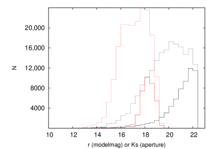
Figure 17: — The magnitude distributions of reliable ${\textit{K}_{s}}$ counterparts to SPIRE sources without reliable optical counterparts. The black histograms show $r$ (modelmag, AB) distributions, the red histograms show ${\textit{K}_{s}}$ (aperture, Vega) magnitude distributions. The dashed histograms represent all reliable counterparts. The black solid line shows the r magnitude distribution of the non-reliable optical matches to SPIRE sources with reliable ${\textit{K}_{s}}$ counterpart. The red solid line shows the distribution of ${\textit{K}_{s}}$ magnitudes of optical drop-outs with reliable ${\textit{K}_{s}}$ counterpart.

It is interesting to consider for how many SPIRE sources the VIKING and SDSS matching disagree on reliable counterparts. 7563 SPIRE sources ($\sim 88\%$ of the reliable optical matches in the VIKING area, $\sim 67\%$ of the reliable VIKING matches) are matched reliably in both surveys. Here, 7404 are matched to the same object. This leaves only 159 SPIRE sources (2.1% of matches) where the identification disagrees. Some of those are deblending issues; often though we find that the reliable optical counterpart is too faint in the ${\textit{K}_{s}}$ band and/or the VIKING counterpart is too faint or not detected in the $r$-band, resulting in different identifications. Fig. 18 shows an example, HATLAS J090550.5+002216.

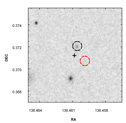
Figure 18: — VIKING ${\textit{K}_{s}}$ image of HATLAS J090550.5+002216, 30” on the side. The black cross marks the SPIRE position. Red circle: reliable SDSS counterpart ($R=0.85$), black circle: reliable VIKING counterpart ($R=0.96$). In the optical, the VIKING counterpart is detected with $r=23.16$, fainter than the limit of $r=22.4$ used in the matching by Smith et al. (2011a).

6.2 Stellar counterparts

Of our 12 reliable stellar matches, 7 have reliable SDSS counterparts. Here, 2 have been classified as galaxies in the Phase 1 catalogue, HATLAS J091233.9-004549 and HATLAS J085353.2+001648 (10930 and 21662 in Fig. 11). Both are clearly stellar, showing diffraction spikes in both SDSS and VIKING images. The reliabilities of the stellar matches to the remaining 5 sources are high with $0.43<R<0.78$.

Conversely, in the optical catalogue there are 21 reliable stellar matches: of these, 19 are in the VIKING area, of which 5 are matched reliably to a VIKING star, 7 stellar objects are not included in our VIKING sample due to saturation in ${\textit{K}_{s}}$, and 7 more are matched, but do not reach $R>0.8$ (but have reliabilities $>0.4$).

6.3 Photometric redshift comparison

Due to the facts that we match with SDSS to obtain our photometry and that ANNz is used in both cases, it is no surprise that the photometric redshift distributions of the reliable counterparts are broadly similar, see Fig. 19. We obtain a slightly higher median redshift of $\tilde{z}=0.396$ compared to the median of $\tilde{z}=0.326$ of the photometric redshifts supplied with the Phase 1 catalogue, partly due to a higher number of redshifts $z_{phot}>1$. Of the 309 SPIRE sources with VIKING reliable counterparts and $z_{phot}>1$, 76 are reliable, have photometric redshifts and are matched to the same object in the optical catalogue. The photometric redshifts of those 76 objects differ by an average of 0.46. This large difference could be explained by incomplete photometric information from UKIDSS LAS used to compile the photometric redshifts in the optical catalogue. Indeed, nearly half (35) of the 76 objects have only 1 or 2 bands in the near-infrared available from LAS. This shows the advantage of the deeper VIKING data. Much better results should be achieved once we have optical photometry from the VST KIDS survey to combine with VIKING.

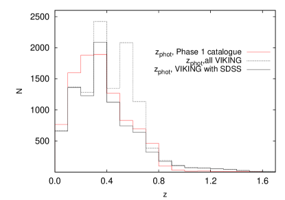
Figure 19: — Comparison of the photometric redshift distributions obtained in this work (VIKING) and supplied with the Phase 1 catalogue. The red line shows the latter, 9583 photometric redshifts with a median of $\tilde{z}=0.326$. The black dashed line shows the former, 11,294 photometric redshifts with a median of $\tilde{z}=0.396$. The black line represents photometric redshifts of the 8748 VIKING objects with SDSS counterparts.

7 Conclusions

We have matched the 22,000 SPIRE G09 sources that fall within the VIKING observed area to a catalogue of near-infrared objects from VIKING: the VIKING sample contains 1,376,606 objects, classified into 847,530 galaxies and 529,076 stars according to shape and colour parameters using a modified version of the method of Baldry et al. (2010). We found statistically, using blank-field comparisons, that $73\pm 2\%$ of SPIRE sources should have one or more counterpart detections in VIKING. With a search radius of $10^{\prime\prime}$ we found 35,800 candidate matches: applying a likelihood ratio method to calculate the probability of each candidate to be the true counterpart of the SPIRE source, we find matches to 11,294 sources ($51.3\%$) with a probability $>80\%$, or reliability $R>0.8$. The false identification rate is estimated to be 4.2% and the probability of mis-identifying a true counterpart is $\sim 5\%$.

Of the reliable counterparts, 3147 (27.9%) have spectroscopic redshifts from either the GAMA or the SDSS redshift surveys. We calculate photometric redshifts for the remaining possible matches, using a sample of 32,465 spectroscopic redshifts as a training set. The errors in the redshift estimation are investigated using the existing 3147 spectroscopic redshifts. We find a scatter of $\sigma=0.0353$ in the difference $|z_{spec}-z_{phot}|$ which is comparable with $\sigma=0.037$ found by Smith et al. (2011a) when calculating photometric redshifts from SDSS/UKIDSS LAS photometry for the HATLAS SDP field. For $z\gtrsim 0.3$ we find that photometric redshifts are systematically underestimated with a bias of $\sim 0.09$.

Comparing our results with that from the $r$-band matching to SDSS objects supplied with the SPIRE catalogue, we report a $\gtrsim 12\%$ increase in the reliable identification rate. We find that we agree on reliable counterparts for $\sim 88\%$ of the reliable optical matches to sources within the VIKING area of the G09 field.

The identifications here provide a useful potential preselection for follow-up studies: the moderate-reliability matches could mostly be confirmed or rejected using optical multi-object spectroscopy, giving a mostly complete subsample for sources at $z<1$; while the $\sim 28\%$ of sources with no match or low-reliability match(es) have a high probability of being at $z>1$, and form a large sample of interesting targets for ALMA $870\,\mu{\rm m}$ snapshots.

A future SPIRE source catalogue will include the VIKING ZYJH${\textit{K}_{s}}$ photometry (aperture magnitudes) for all candidate matches, but we stress that only matches with $R>0.8$ should be regarded as reliable counterparts and used for science application.

8 Acknowledgements

We thank the anonymous referee for useful comments.

The Herschel-ATLAS is a project with Herschel, which is an ESA space observatory with science instruments provided by European-led Principal Investigator consortia and with important participation from NASA. The H-ATLAS website is http://www.h-atlas.org/ U.S. participants in Herschel ATLAS acknowledge support provided by NASA through a contract issued from JPL.

GAMA is a joint European-Australasian project based around a spectroscopic campaign using the Anglo-Australian Telescope. The GAMA input catalogue is based on data taken from the Sloan Digital Sky Survey and the UKIRT Infrared Deep Sky Survey. Complementary imaging of the GAMA regions is being obtained by a number of independent survey programs including GALEXMIS, VST KIDS, VISTA VIKING,WISE, Herschel-ATLAS, GMRT and ASKAP providing UV to radio coverage. The GAMA website is: http://www.gama-survey.org/. This work used data from the UKIDSS DR5 and the SDSS DR7. The UKIDSS project is defined in Lawrence et al. (2007) and uses the UKIRTWide Field Camera (WFCAM; Casali et al. 2007). Funding for the SDSS and SDSS-II has been provided by the Alfred P. Sloan Foundation, the Participating Institutions, The National Science Foundation, the U.S. Department of Energy, the National Aeronautics and Space Administration, the Japanese Monbukagakusho, the Max Planck Society and the Higher Education Funding Council for England.

The Italian group acknowledges partial financial support from ASI contract I/009/10/0 COFIS .

This work used data from VISTA at the ESO Paranal Observatory, programme 179.A-2004. VISTA is an ESO near-infrared survey telescope in Chile, conceived and developed by a consortium of universities in the United Kingdom, led by Queen Mary University, London.

APPENDIX: Images

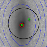
(A1.1)

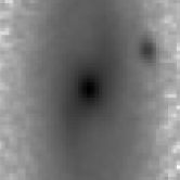
(A1.2)

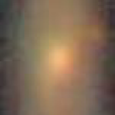
(A1.3)

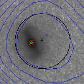
(A1.4)

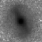
(A1.5)

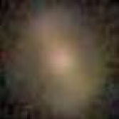
(A1.6)

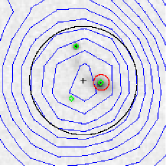
(A1.7)

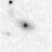
(A1.8)

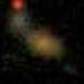
(A1.9)

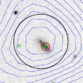
(A1.10)

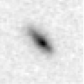
(A1.11)

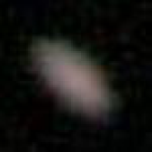
(A1.12)

Figure A1: VIKING and SDSS cutouts of a random selection of SPIRE positions. The image on the left shows a 30” VIKING cutout; the possible counterparts are indicated with a green diamond, the reliable counterpart is encircled in red. The black (or white) cross shows the SPIRE position and the black circle represents the search radius of 10”. The middle image shows a 15” VIKING cutout centered on the position of the reliable counterpart. The image on the right shows a 15” SDSS cutout centered on the position of the reliable VIKING counterpart. On all images, North is up and East is left.

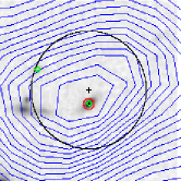
(A1.13)

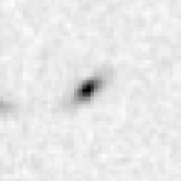
(A1.14)

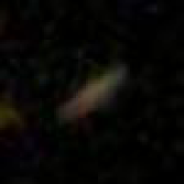
(A1.15)

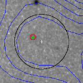
(A1.16)

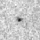
(A1.17)

(A1.18)

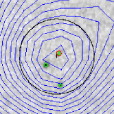
(A1.19)

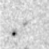
(A1.20)

(A1.21)

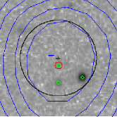
(A1.22)

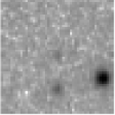
(A1.23)

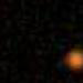
(A1.24)

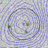
(A1.25)

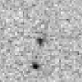
(A1.26)

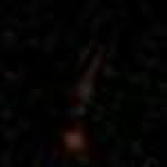
(A1.27)

Figure A1: continued

References

- Amblard et al. (2010) Amblard A. et al., 2010, A&A, 518, L9
- Baldry et al. (2010) Baldry I.K. et al., 2010, MNRAS, 404, 86
- Bell et al. (2003) Bell E.F., McIntosh D.H., Katz N., Weinberg M., 2003, ApJS, 149, 289
- Bell et al. (2006) Bell E.F., Phleps S., Somerville R.S., Wolf C., Borch A., Meisenheimer K., 2006, ApJ, 652, 270
- Biggs et al. (2011) Biggs A.D. et al., 2011, MNRAS, 413, 2314
- Blain & Longair (1993) Blain A.W., Longair M.S., 1993, MNRAS, 264, 509
- Bond et al. (submitted to ApJL) Bond N. et al., submitted to ApJL
- Bourne et al. (2011) Bourne N. et al., 2011, MNRAS, 410, 1155
- Chapin et al. (2011) Chapin E.L. et al., 2011, MNRAS, 411, 505
- Ciliegi et al. (2003) Ciliegi P., Zamorani G., Hasinger G., Lehmann I., Szokoly G., Wilson G., 2003, A&A, 398, 901
- Ciliegi et al. (2005) Ciliegi P. et al., 2005, A&A, 441, 879
- Cole et al. (2001) Cole S. et al., 2001, MNRAS, 326, 255
- Collister & Lahav (2004) Collister A., Lahav O., 2004, PASP, 116, 818, 345
- DeBoer et al. (2009) DeBoer D.R., 2009, Proc. IEEE, 97, 1507
- de Ruiter, Arp & Willis (1977) de Ruiter H.R., Arp H. C., Willis A. G., 1977, A&AS, 28, 211
- Dariush et al. (2011) Dariush A. et al., 2011, MNRAS, 418, 64
- Davis et al. (2003) Davis M. et al., 2003, Proc. SPIE, 4834, 161
- Devlin et al. (2009) Devlin M. et al., 2009, Nature, 458, 737
- Driver et al. (2011) Driver S.P. et al., 2011, MNRAS, 412,765
- Dunlop et al. (2010) Dunlop J.S. et al., 2010, MNRAS, 408, 2022
- Dye et al. (2009) Dye S. et al., 2009, ApJ, 703, 285
- Dye et al. (2010) Dye S. et al., 2010, A&A, 518, L10
- Eales et al. (2010) Eales S.A. et al., 2010, PASP, 122, 499
- Elbaz et al. (2010) Elbaz D. et al., 2010, A&A, 518, L29
- Emerson et al. (2004) Emerson J.P. et al., 2004, Proc. SPIE, 5493, 401
- Emerson & Sutherland (2010) Emerson J.P., Sutherland W.J., 2010, Proc. SPIE, 7733, 4
- Findlay et al. (2012) Findlay, J. R., Sutherland, W. J., Venemans, B. P., Reylé, C., Robin, A. C., Bonfield, D. G., Bruce, V. A., Jarvis, M. J., MNRAS, 419, 3354
- Fukugita et al. (1996) Fukugita M., Ichikawa, T., Gunn, J.E., Doi, M., Shimasaku, K., Schneider, D.P., 1996, AJ, 111, 1748
- Gonzáles-Nuevo et al. (2010) Gonzáles-Nuevo J. et al., 2010, A&A, 518, L38
- Griffin et al. (2010) Griffin M.J. et al., 2010, A&A, 518, L3
- Hainline et al. (2010) Hainline L.J. et al., 2010, AAS 21532601, 42, 422
- Hambly et al. (2008) Hambly N. et al., 2008, MNRAS, 384, 637
- Hardcastle et al. (2010) Hardcastle M.J. et al., 2010, MNRAS, 409, 122
- Helou et al. (1985) Helou G., Soifer B.T., Rowan-Robinson M., 1985, ApJ, 298, 7
- Hewitt et al. (2006) Hewitt P.C. et al., 2006, MNRAS, 367, 454
- Hoyos et al. (in prep.) Hoyos C. et al., in preparation
- Ibar et al. (2010) Ibar E. et al., 2010, MNRAS, 409, 38
- Ivison et al. (2007) Ivison R.J. et al., 2007, MNRAS, 380, 199
- Ivison et al. (2010) Ivison R.J. et al., 2010, A&A, 518, L31
- Jarvis et al. (2010) Jarvis M. et al., 2010, MNRAS, 409, 92
- Johnston et al. (2008) Johnston S. et al., 2008, Experimental Astronomy, 22, Issue 3, 151
- Kim et al. (submitted to ApJ) Kim S. et al., submitted to ApJ, arXiv:1112.3653
- Lagache et al. (2003) Lagache G., Dole H., Puget J.-L., 2003, MNRAS, 338, 555
- Lapi et al. (2011) Lapi A. et al., ApJ, 742, 24
- Lawrence et al. (2010) Lawrence A. et al., 2007, MNRAS, 379, 1599
- Lewis, Irwin & Bunclark (2010) Lewis J.R., Irwin M., Bunclark P., 2010, ASPC, 434, 91L
- Lilly et al. (2007) Lilly S.J., 2007, ApJS, 172, 70
- Lotz (2007) Lotz J.M., 2007, ASPC, 380, 467
- Maddox et al. (2010) Maddox S.J. et al., 2010, A&A, 518, L11
- Michalowski, Watson & Hjorth (2010) Michalowski M.J., Watson D. and Hjorth J. 2010, ApJ, 712, 942
- Mortier et al. (2005) Mortier A.M.J. et al., 2005, MNRAS, 363, 563
- Negrello et al. (2007) Negrello M. et al., 2007, MNRAS, 377, 1557
- Negrello et al. (2010) Negrello M. et al., 2010, Sci, 330, 800
- Norris et al. (2011) Norris R.P. et al., 2011, PASA, 28, 215
- Oliver et al. (2010) Oliver M. et al., 2010, A&A 518, L21
- Pascale et al. (2010) Pascale E. et al., 2011, MNRAS, 415, 911
- Pilbratt et al. (2010) Pilbratt G.L. et al., 2010, A&A, 518 L1
- Poglitsch et al. (2010) Poglitsch A. et al., 2010, A&A, 518, L2
- Prestage & Peacock (1983) Prestage R.M., Peacock J. A., 1983, MNRAS, 204, 355
- Rigby et al. (2011) Rigby E.E. et al., 2011, MNRAS, 415, 3
- Rodighiero et al. (2010) Rodighiero G. et al., 2010, A&A 518, L25
- Roseboom et al. (2010) Roseboom I.G. et al., 2010, MNRAS, 409, 48
- Ryan et al. (2008) Ryan R.E., Cohen S.H., Windhorst R.A., Silk J., 2008, ApJ, 678, 751
- Schilizzi, Dewdney & Lazio (2008) Schilizzi Richard T., Dewdney Peter E.F., Lazio T. Joseph W., 2008, Proc. SPIE, 7012, 52
- Serjeant et al. (2003) Serjeant S. et al., 2003, MNRAS, 334, 887
- Smail, Ivison & Blain (1997) Smail I., Ivison R.J., Blain A.W., 1997, ApJ, 490, L5
- Smith et al. (2011a) Smith D.J.B. et al., 2011a, MNRAS, 416, 857
- Smith et al. (2011b) Smith D.J.B. et al., 2011b, submitted to MNRAS