Landau theory for the phase diagram of the multiferroic $\textbf{Mn}_{\textbf{{1-x}}}\textbf{(Fe,Zn,Mg)}_{\textbf{{x}}}\textbf{WO}_{\textbf{{4}}}$

Abstract

We present a theoretical analysis of the temperature-magnetic field-concentration phase diagram of the multiferroic Mn_1-xM_xWO₄ (M=Fe, Zn, Mg), which exhibits three ordered phases, with collinear and non-collinear incommensurate and with a commensurate magnetic order. The middle phase is also ferroelectric. The analysis uses a semi-phenomenological Landau theory, based on a Heisenberg Hamiltonian with a single-ion anisotropy. With a small number of adjustable parameters, the Landau theory gives an excellent fit to all three transition lines, as well as the magnetic and the ferroelectric order parameters. The fit of the magnetic and ferroelectric order parameters is further improved by including the effect of fluctuations near the transitions. We demonstrate the highly frustrated nature of these materials and suggest a simple explanation for the dramatic effects of doping with different magnetic ions at the Mn sites. The model enables an examination of different sets of exchange couplings that were proposed by a number of groups. Small discrepancies are probably a consequence of small errors in the experimental magnetic parameters. In addition, using the Ginzburg criterion we estimate the temperature range in which fluctuations of the order parameters become important.

I Introduction

Type II Magnetoelectric multiferroics are materials which exhibit coexistence between certain types of long-range magnetic order and a ferroelectric order. These materials are usually characterized by a strong magnetoelectric coupling between their electric and magnetic degrees of freedom. The magnetoelectric effect enables the control of the electric polarization by a magnetic field, or the control of the magnetization by an electric field. The study of magnetoelectric multiferroics is thus of great interest in condensed matter physics, both from basic research and technological applications points of view.KD09 ; CSW07 ; FM05 ; KT07 In recent years, the interest in this field has grown after the discovery of new materials with a large magnetoelectric effect, such as TbMnO₃,KT03 TbMn₂O₅,HN04 Ni₃V₂O₈,LG05 CuFeO₂,KT06 and CoCr₂O₄.YY06 In those oxides, ferroelectricity appears in conjunction with a noncollinear spiral magnetic phase, which breaks spatial inversion symmetry, and therefore allows the appearance of an electric polarization.

There are two different approaches to the theoretical treatment of such noncollinear magnetoelectric multiferroics. One approach is based on first principles calculations using the density functional theory (DFT).PS09 The second approach constructs a model Hamiltonian dictated by symmetry considerations.LG05 ; MM06 ; HAB07 Different mechanisms for the magnetoelectric coupling can then be suggested.HAB06 ; KD09 ; KH05 ; SI06 In this paper we develop a semi-phenomenological model for describing the magnetic phase transitions of Mn_1-xM_xWO₄ (M=Fe, Zn, Mg) and the induced ferroelectric polarization. The model is semi-phenomenological in the sense that some of the parameters can be deduced from existing experimental data, while the others are purely phenomenological. The multiferroic MnWO₄ is a natural choice for such an approach, due to the vast experimental data that exists in the literature.

MnWO₄ crystallizes in the wolframite structure, which belongs to the monoclinic space group P2/c with $\beta\approx 91\degree$. The unit cell includes two magnetic Mn²⁺ ions with spin $S=5/2$ and orbital angular momentum $L=0$ at positions $\mbox{\boldmath{$\tau$}}_{1}=(0.5,y,0.25)$ and $\mbox{\boldmath{$\tau$}}_{2}=(0.5,1-y,0.75)$ (in units of the primitive lattice vectors) with $y=0.685$.LG93 In zero magnetic field, MnWO₄ undergoes three successive phase transitions at temperatures $T_{N3}\approx 13.5K$, $T_{N2}\approx 12.3-12.7K$ and $T_{N1}\approx 7-8K$ to phases which are called AF3, AF2, and AF1, respectively.LG93 ; AAH06 ; TK06 According to neutron diffraction experiments,LG93 AF3 is an incommensurate (IC) antiferromagnetic phase with a collinear sinusoidal structure, AF2 is an incommensurate antiferromagnetic phase with an elliptical-spiral structure, and AF1 is a commensurate (C) antiferromagnetic phase with a collinear $\uparrow\uparrow\downarrow\downarrow$ structure. The propagation vectors are $\mbox{\boldmath{$q$}}_{IC}=(-0.214,0.5,0.457)$ (in units of the primitive reciprocal lattice vectors) for AF2 and AF3, and $\mbox{\boldmath{$q$}}_{C1,2}=(\pm 0.25,0.5,0.5)$ for AF1. In AF3 and AF1, the magnetic moments of the Mn²⁺ ions align along the easy axis of magnetization, which lies in the $ac$-plane and forms an angle of $\approx 35\degree-37\degree$ with the $a$ axis. Different studiesAAH06 ; TK06 reveal that a ferroelectric polarization, which is oriented along the $b$ axis, develops in the AF2 phase.

As opposed to MnWO₄, other isomorphic wolframite structures like FeWO₄, CoWO₄ and NiWO₄ show only a single magnetic phase transition to a simple commensurate antiferromagnetic phase with the propagation vector $\mbox{\boldmath{$q$}}=(0.5,0,0)$.WH77 Those observations suggest that unlike the isomorphic structures, MnWO₄ constitutes a highly frustrated system with complex competing interactions. The competition between the different interactions manifests itself in the sensitivity of the phase diagram to doping with different transition metal ions at the Mn sites. It turns out that a small Fe concentration suppresses the ferroelectric phase AF2 and expands the stabilization range of AF3 and AF1.CRP09 ; YF08 ; CRP08 In contrast to Fe doping, it has been reportedSYS09 that a small Co concentration stabilizes the ferroelectric phase at the expense of the AF1 phase. A quantitative and microscopic understanding of the effect of Fe and Co doping on the multiferroic properties and the phase diagram of MnWO₄ is quite complicated, since the exchange couplings of the M-M and M-Mn (M=Fe, Co) interactions, as well as the anisotropy parameters are not known. In order to overcome some of these problems, a much simpler magnetic system has been achieved by the partial substitution of Mn ions by the non-magnetic ions Zn²⁺ and Mg²⁺.CRP11 ; ML09 Those studies reveal that the AF1 phase is strongly suppressed as a result of magnetic ions dilution by non-magnetic substituents.

The frustrated nature of MnWO₄ was demonstrated by Ehrenberg et al..EH99 Using inelastic neutron scattering they extracted 9 exchange couplings $J_{1}-J_{9}$ for the superexchange interactions among the Mn ions. Later, Tian et al.TC09 proposed different values for the 9 exchange couplings based on DFT calculations. Those values depend on an unknown on-site repulsion energy. Moreover, the authors have noted that generally DFT calculations tend to overestimate the magnitude of exchange interactions.TC09 Recently, the experimental data have been expanded.YF11 In that study, Ye et al. suggested some corrections for the values of the exchange couplings, and included two additional ones, $J_{10}$ and $J_{11}$. The two sets of experimental exchange couplings are summarized in Table  1. The model we describe may help to compare these different sets of exchange couplings, by examining their consistency with different experimental observations.

Table 1: Superexchange couplings for the Mn²⁺ ion at $\mbox{\boldmath{$\tau$}}_{1}=(0.5,y,0.25)$ according to different inelastic neutron scattering studies. We denote $z=1-y$, $w=2-y$ and $u=1+y$. The values are presented in units of $k_{B}K$.comment1

$J_{1}$

$J_{2}$

$J_{3}$

$J_{4}$

$J_{5}$

$J_{6}$

$J_{7}$

$J_{8}$

$J_{9}$

$J_{10}$

$J_{11}$

D

Neighbors

$\left(\frac{1}{2},z,\frac{3}{4}\right)$

$\left(\frac{1}{2},w,\frac{3}{4}\right)$

$\left(\frac{3}{2},y,\frac{1}{4}\right)$

$\left(\frac{1}{2},y,\frac{5}{4}\right)$

$\left(\frac{1}{2},u,\frac{1}{4}\right)$

$\left(\frac{3}{2},z,\frac{3}{4}\right)$

$\left(-\frac{1}{2},z,\frac{3}{4}\right)$

$\left(\frac{3}{2},w,\frac{3}{4}\right)$

$\left(-\frac{1}{2},w,\frac{3}{4}\right)$

$\left(\frac{3}{2},y,\frac{5}{4}\right)$

$\left(\frac{3}{2},y,-\frac{3}{4}\right)$

$\left(\frac{1}{2},z,-\frac{1}{4}\right)$

$\left(\frac{1}{2},w,-\frac{1}{4}\right)$

$\left(-\frac{1}{2},y,\frac{1}{4}\right)$

$\left(\frac{1}{2},y,-\frac{3}{4}\right)$

$\left(\frac{1}{2},-z,\frac{1}{4}\right)$

$\left(-\frac{1}{2},z,-\frac{1}{4}\right)$

$\left(\frac{3}{2},z,-\frac{1}{4}\right)$

$\left(\frac{3}{2},w,-\frac{1}{4}\right)$

$\left(\frac{3}{2},w,-\frac{1}{4}\right)$

$\left(-\frac{1}{2},y,-\frac{3}{4}\right)$

$\left(-\frac{1}{2},y,\frac{5}{4}\right)$

Ref. EH99,

-0.195

-0.135

-0.423

0.414

0.021

-0.509

0.023

0.491

-1.273

-

-

0.568

Ref. YF11,

-1.95(1)

-0.18(1)

-1.48(1)

-1.21(1)

0.23(1)

-1.99(1)

-0.56(1)

0.09(1)

-1.21(1)

-0.7(1)

0.09(1)

0.84(1)

The outline of the paper is as follows: in Sec. II we define the model. In Sec. III the results of the model are derived. In Sec. IV the model parameters are fitted by comparing its results with different experimental observations. Here we compare the two sets of experimental exchange couplings with the fitted parameters. In Sec. V the Ginzburg criterion is applied to the specific case of the multiferroic MnWO₄, in order to examine whether the mean-field theory approach is valid. We conclude in Sec. VI with a brief summary.

II The model

In this section we develop the semi-phenomenological model. The spin Hamiltonian consists of a Heisenberg term with a single-ion anisotropy, which favors an easy axis in the $ac$-plane. According to experiments, the spin component along the hard axis in the $ac$-plane does not order in any of the phases. Furthermore, the transitions are almost not influenced by an external magnetic field along the hard axis. Hence we omit the hard axis component from the calculations and write the spin as $\mbox{\boldmath{$S$}}(\mbox{\boldmath{$R$}}+\mbox{\boldmath{$\tau$}})=S_{x}(\mbox{\boldmath{$R$}}+\mbox{\boldmath{$\tau$}})\hat{\bf x}+S_{b}(\mbox{\boldmath{$R$}}+\mbox{\boldmath{$\tau$}})\hat{\bf b}$, where $x$ denotes the easy axis in the $ac$-plane and $b$ denotes the axis perpendicular to the $ac$-plane. Here $\mbox{\boldmath{$S$}}(\mbox{\boldmath{$R$}}+\mbox{\boldmath{$\tau$}})$ is the thermal average of the dimensionless classical spin at position $\mbox{\boldmath{$R$}}+\mbox{\boldmath{$\tau$}}$, where $R$ is a lattice vector and $\tau$ is one of the two basis vectors $\mbox{\boldmath{$\tau$}}_{1}$, $\mbox{\boldmath{$\tau$}}_{2}$ in the unit cell, indicating the locations of the Mn²⁺ ions. We study the following Hamiltonian:

$$H_{mag}=-\frac{1}{2}\sum_{\mbox{\boldmath{$R$}},\mbox{\boldmath{$R$}}^{\prime}}\sum_{\mbox{\boldmath{$\tau$}},\mbox{\boldmath{$\tau$}}^{\prime}=\mbox{\boldmath{$\tau$}}_{1},\mbox{\boldmath{$\tau$}}_{2}}J(\mbox{\boldmath{$R$}}+\mbox{\boldmath{$\tau$}},\mbox{\boldmath{$R$}}^{\prime}+\mbox{\boldmath{$\tau$}}^{\prime})\mbox{\boldmath{$S$}}(\mbox{\boldmath{$R$}}+\mbox{\boldmath{$\tau$}})\cdot\mbox{\boldmath{$S$}}(\mbox{\boldmath{$R$}}^{\prime}+\mbox{\boldmath{$\tau$}}^{\prime})-\frac{1}{2}D\sum_{\mbox{\boldmath{$R$}}}\sum_{\mbox{\boldmath{$\tau$}}=\mbox{\boldmath{$\tau$}}_{1},\mbox{\boldmath{$\tau$}}_{2}}{S_{x}}^{2}(\mbox{\boldmath{$R$}}+\mbox{\boldmath{$\tau$}}).$$ (1)

Here $J(\mbox{\boldmath{$R$}}+\mbox{\boldmath{$\tau$}},\mbox{\boldmath{$R$}}^{\prime}+\mbox{\boldmath{$\tau$}}^{\prime})$ is the superexchange interaction energy which couples the spins at $\mbox{\boldmath{$R$}}+\mbox{\boldmath{$\tau$}}$ and $\mbox{\boldmath{$R$}}^{\prime}+\mbox{\boldmath{$\tau$}}^{\prime}$, and $D$ is a positive single-ion anisotropy energy. To find an expression for the magnetic free energy of the system, we expand the entropy in the spin components up to the fourth order

$$T\texttt{S} =-\frac{1}{2}aT\sum_{\mbox{\boldmath{$R$}}}\sum_{\mbox{\boldmath{$\tau$}}=\mbox{\boldmath{$\tau$}}_{1},\mbox{\boldmath{$\tau$}}_{2}}{\mbox{\boldmath{$S$}}}^{2}(\mbox{\boldmath{$R$}}+\mbox{\boldmath{$\tau$}})$$

$$-b\sum_{\mbox{\boldmath{$R$}}}\sum_{\mbox{\boldmath{$\tau$}}=\mbox{\boldmath{$\tau$}}_{1},\mbox{\boldmath{$\tau$}}_{2}}{\mbox{\boldmath{$S$}}}^{4}(\mbox{\boldmath{$R$}}+\mbox{\boldmath{$\tau$}}),$$ (2)

where $a$ and $b$ are positive parameters, and $T$ is the temperature. Equation (II) gives the entropy relative to the high temperature paramagnetic phase (denoted by P) and thus the expression is negative. Combining Eqs. (1) and (II) we obtain the magnetic free energy

$$F_{mag}=\frac{1}{2}\sum_{\mbox{\boldmath{$R$}},\mbox{\boldmath{$R$}}^{\prime}}\sum_{\mbox{\boldmath{$\tau$}},\mbox{\boldmath{$\tau$}}^{\prime}=\mbox{\boldmath{$\tau$}}_{1},\mbox{\boldmath{$\tau$}}_{2}}\sum_{\alpha,\beta=1}^{2}\chi^{-1}_{\alpha\beta}(\mbox{\boldmath{$R$}}+\mbox{\boldmath{$\tau$}},\mbox{\boldmath{$R$}}^{\prime}+\mbox{\boldmath{$\tau$}}^{\prime})S_{\alpha}(\mbox{\boldmath{$R$}}+\mbox{\boldmath{$\tau$}})S_{\beta}(\mbox{\boldmath{$R$}}^{\prime}+\mbox{\boldmath{$\tau$}}^{\prime})+b\sum_{\mbox{\boldmath{$R$}}}\sum_{\mbox{\boldmath{$\tau$}}=\mbox{\boldmath{$\tau$}}_{1},\mbox{\boldmath{$\tau$}}_{2}}{\mbox{\boldmath{$S$}}}^{4}(\mbox{\boldmath{$R$}}+\mbox{\boldmath{$\tau$}}),$$ (3)

where the $4\times 4$ inverse susceptibility matrix is block diagonal

$$\chi^{-1}_{\alpha\beta}(\mbox{\boldmath{$R$}}+\mbox{\boldmath{$\tau$}},\mbox{\boldmath{$R$}}^{\prime}+\mbox{\boldmath{$\tau$}}^{\prime}) =\big{[}(aT-D_{\alpha})\delta_{\mbox{\boldmath{$R$}},\mbox{\boldmath{$R$}}^{\prime}}\delta_{\tau,\tau^{\prime}}$$

$$-J(\mbox{\boldmath{$R$}}+\mbox{\boldmath{$\tau$}},\mbox{\boldmath{$R$}}^{\prime}+\mbox{\boldmath{$\tau$}}^{\prime})\big{]}\delta_{\alpha,\beta},$$ (4)

with $D_{1}=D_{x}=D$ and $D_{2}=D_{b}=0$. Below, we exploit the Fourier transforms of the spin components,

$$S_{\alpha}(\mbox{\boldmath{$q$}},\mbox{\boldmath{$\tau$}})=\frac{1}{N}\sum_{\mbox{\boldmath{$R$}}}S_{\alpha}(\mbox{\boldmath{$R$}}+\mbox{\boldmath{$\tau$}})e^{i\mbox{\boldmath{$q$}}\cdot(\mbox{\boldmath{$R$}}+\mbox{\boldmath{$\tau$}})},$$

$$S_{\alpha}(\mbox{\boldmath{$R$}}+\mbox{\boldmath{$\tau$}})=\sum_{\mbox{\boldmath{$q$}}}S_{\alpha}(\mbox{\boldmath{$q$}},\mbox{\boldmath{$\tau$}})e^{-i\mbox{\boldmath{$q$}}\cdot(\mbox{\boldmath{$R$}}+\mbox{\boldmath{$\tau$}})}.$$ (5)

Here $q$ is in the first Brillouin zone and $N$ is the number of unit cells. In terms of the Fourier transform, the magnetic free energy per unit cell, $f_{mag}\equiv{F_{mag}/N}$, is:

$$f_{mag} =\frac{1}{2}\sum_{\mbox{\boldmath{$\tau$}},\mbox{\boldmath{$\tau$}}^{\prime}=\mbox{\boldmath{$\tau$}}_{1},\mbox{\boldmath{$\tau$}}_{2}}\sum_{\alpha,\beta=1}^{2}\sum_{\mbox{\boldmath{$q$}}}\chi^{-1}_{\alpha\beta}(\mbox{\boldmath{$q$}};\mbox{\boldmath{$\tau$}},\mbox{\boldmath{$\tau$}}^{\prime}){S_{\alpha}}^{\ast}(\mbox{\boldmath{$q$}},\mbox{\boldmath{$\tau$}})S_{\beta}(\mbox{\boldmath{$q$}},\mbox{\boldmath{$\tau$}}^{\prime})$$

$$+b\sum_{\mbox{\boldmath{$G$}}}\sum_{\mbox{\boldmath{$\tau$}}=\mbox{\boldmath{$\tau$}}_{1},\mbox{\boldmath{$\tau$}}_{2}}\sum_{\mbox{\boldmath{$q$}}_{1},\mbox{\boldmath{$q$}}_{2},\mbox{\boldmath{$q$}}_{3},\mbox{\boldmath{$q$}}_{4}}e^{-i\mbox{\boldmath{$G$}}\cdot\mbox{\boldmath{$\tau$}}}\big{[}S_{x}(\mbox{\boldmath{$q$}}_{1},\mbox{\boldmath{$\tau$}})S_{x}(\mbox{\boldmath{$q$}}_{2},\mbox{\boldmath{$\tau$}})S_{x}(\mbox{\boldmath{$q$}}_{3},\mbox{\boldmath{$\tau$}})S_{x}(\mbox{\boldmath{$q$}}_{4},\mbox{\boldmath{$\tau$}})$$

$$+S_{b}(\mbox{\boldmath{$q$}}_{1},\mbox{\boldmath{$\tau$}})S_{b}(\mbox{\boldmath{$q$}}_{2},\mbox{\boldmath{$\tau$}})S_{b}(\mbox{\boldmath{$q$}}_{3},\mbox{\boldmath{$\tau$}})S_{b}(\mbox{\boldmath{$q$}}_{4},\mbox{\boldmath{$\tau$}})+2S_{x}(\mbox{\boldmath{$q$}}_{1},\mbox{\boldmath{$\tau$}})S_{x}(\mbox{\boldmath{$q$}}_{2},\mbox{\boldmath{$\tau$}})S_{b}(\mbox{\boldmath{$q$}}_{3},\mbox{\boldmath{$\tau$}})S_{b}(\mbox{\boldmath{$q$}}_{4},\mbox{\boldmath{$\tau$}})\big{]}\delta(\mbox{\boldmath{$q$}}_{1}+\mbox{\boldmath{$q$}}_{2}+\mbox{\boldmath{$q$}}_{3}+\mbox{\boldmath{$q$}}_{4}-\mbox{\boldmath{$G$}}),$$ (6)

where $G$ is a reciprocal lattice vector and the Fourier transform of the inverse susceptibility matrix is given by the block diagonal hermitian matrix

$$\chi^{-1}_{\alpha\beta}(\mbox{\boldmath{$q$}};\mbox{\boldmath{$\tau$}},\mbox{\boldmath{$\tau$}}^{\prime}) =\big{[}(aT-D_{\alpha})\delta_{\mbox{\boldmath{$\tau$}},\mbox{\boldmath{$\tau$}}^{\prime}}$$

$$-J(\mbox{\boldmath{$q$}};\mbox{\boldmath{$\tau$}},\mbox{\boldmath{$\tau$}}^{\prime})\big{]}\delta_{\alpha,\beta},$$ (7)

with $J(\mbox{\boldmath{$q$}};\mbox{\boldmath{$\tau$}},\mbox{\boldmath{$\tau$}}^{\prime})$ being the Fourier transform of the $2\times 2$ matrix $J(\mbox{\boldmath{$R$}}+\mbox{\boldmath{$\tau$}},\mbox{\boldmath{$R$}}^{\prime}+\mbox{\boldmath{$\tau$}}^{\prime})$

$$J(\mbox{\boldmath{$q$}};\mbox{\boldmath{$\tau$}},\mbox{\boldmath{$\tau$}}^{\prime})=\sum_{\mbox{\boldmath{$R$}}}J(\mbox{\boldmath{$\tau$}},\mbox{\boldmath{$R$}}+\mbox{\boldmath{$\tau$}}^{\prime})e^{-i\mbox{\boldmath{$q$}}\cdot(\mbox{\boldmath{$R$}}+\mbox{\boldmath{$\tau$}}^{\prime}-\mbox{\boldmath{$\tau$}})}.$$ (8)

In the last expression the sum is over all lattice vectors $R$. The four eigenvalues of the matrix (II) are

$$\zeta_{\pm,x}(\mbox{\boldmath{$q$}},T)=aT-D-\lambda_{\pm}(\mbox{\boldmath{$q$}}),$$

$$\zeta_{\pm,b}(\mbox{\boldmath{$q$}},T)=aT-\lambda_{\pm}(\mbox{\boldmath{$q$}}),$$ (9)

and the corresponding eigenvectors are

$$\mbox{\boldmath{$S$}}_{\pm,x}(\mbox{\boldmath{$q$}})=\frac{1}{\sqrt{2}}\begin{pmatrix}1\\ \pm{e}^{-i\phi(\mbox{\boldmath{$q$}})}\\ 0\\ 0\end{pmatrix},$$

$$\mbox{\boldmath{$S$}}_{\pm,b}(\mbox{\boldmath{$q$}})=\frac{1}{\sqrt{2}}\begin{pmatrix}0\\ 0\\ 1\\ \pm{e}^{-i\phi(\mbox{\boldmath{$q$}})}\end{pmatrix}.$$ (10)

Here, $\lambda_{\pm}$ are the two eigenvalues of the matrix (8) and $\phi(\mbox{\boldmath{$q$}})$ is the phase of $J(\mbox{\boldmath{$q$}};1,2)$. Assuming 11 exchange couplings as in Ref. YF11, , these two eigenvalues are given by

$$\lambda_{\pm}(\mbox{\boldmath{$q$}}) =\pm 2\sqrt{{\Lambda_{2}}^{2}(\mbox{\boldmath{$q$}})+{\Lambda_{3}}^{2}(\mbox{\boldmath{$q$}})+2\cos(2\pi q_{b})\Lambda_{2}(\mbox{\boldmath{$q$}})\Lambda_{3}(\mbox{\boldmath{$q$}})}$$

$$+2\Lambda_{1}(\mbox{\boldmath{$q$}}),$$ (11)

with the following definitions:

$$\Lambda_{1}(\mbox{\boldmath{$q$}}) =J_{3}\cos(2\pi q_{a})+J_{4}\cos(2\pi q_{c})$$

$$+J_{5}\cos(2\pi q_{b})+J_{10}\cos\big{[}2\pi(q_{a}+q_{c})\big{]}$$

$$+J_{11}\cos\big{[}2\pi(q_{a}-q_{c})\big{]},$$

$$\Lambda_{2}(\mbox{\boldmath{$q$}}) =J_{1}\cos(\pi q_{c})+J_{6}\cos\big{[}2\pi(q_{a}+\frac{q_{c}}{2})\big{]}$$

$$+J_{7}\cos\big{[}2\pi(q_{a}-\frac{q_{c}}{2})\big{]},$$

$$\Lambda_{3}(\mbox{\boldmath{$q$}}) =J_{2}\cos(\pi q_{c})+J_{8}\cos\big{[}2\pi(q_{a}+\frac{q_{c}}{2})\big{]}$$

$$+J_{9}\cos\big{[}2\pi(q_{a}-\frac{q_{c}}{2})\big{]}.$$ (12)

Now let us transform to magnetic normal coordinates

$$\begin{pmatrix}S_{x}(\mbox{\boldmath{$q$}},1)\\ S_{x}(\mbox{\boldmath{$q$}},2)\\ S_{b}(\mbox{\boldmath{$q$}},1)\\ S_{b}(\mbox{\boldmath{$q$}},2)\end{pmatrix} =\sigma_{+,x}(\mbox{\boldmath{$q$}})\mbox{\boldmath{$S$}}_{+,x}(\mbox{\boldmath{$q$}})+\sigma_{-,x}(\mbox{\boldmath{$q$}})\mbox{\boldmath{$S$}}_{-,x}(\mbox{\boldmath{$q$}})$$

$$+\sigma_{+,b}(\mbox{\boldmath{$q$}})\mbox{\boldmath{$S$}}_{+,b}(\mbox{\boldmath{$q$}})+\sigma_{-,b}(\mbox{\boldmath{$q$}})\mbox{\boldmath{$S$}}_{-,b}(\mbox{\boldmath{$q$}}).$$ (13)

Here, $\sigma_{+,x}(\mbox{\boldmath{$q$}})$, $\sigma_{-,x}(\mbox{\boldmath{$q$}})$, $\sigma_{+,b}(\mbox{\boldmath{$q$}})$ and $\sigma_{-,b}(\mbox{\boldmath{$q$}})$ are the magnetic order parameters for a magnetic structure with wave vector $q$. The diagonal form of the magnetic free energy (II) is therefore

$$f_{mag} =\frac{1}{2}\sum_{\mbox{\boldmath{$q$}}}\big{[}\zeta_{+,x}(\mbox{\boldmath{$q$}},T)\left|\sigma_{+,x}(\mbox{\boldmath{$q$}})\right|^{2}+\zeta_{-,x}(\mbox{\boldmath{$q$}},T)\left|\sigma_{-,x}(\mbox{\boldmath{$q$}})\right|^{2}$$

$$+\zeta_{+,b}(\mbox{\boldmath{$q$}},T)\left|\sigma_{+,b}(\mbox{\boldmath{$q$}})\right|^{2}+\zeta_{-,b}(\mbox{\boldmath{$q$}},T)\left|\sigma_{-,b}(\mbox{\boldmath{$q$}})\right|^{2}\big{]}$$

$$+O({\sigma}^{4}).$$ (14)

At high enough temperatures, the eigenvalues (II) are all positive and therefore the stable phase is the paramagnetic one. As we lower the temperature, we reach a critical temperature for which one of the eigenvalues vanishes. We denote the wave vector for which one of the eigenvalues vanishes first as $\mbox{\boldmath{$q$}}_{IC}$. Since $\lambda_{+}(\mbox{\boldmath{$q$}})>\lambda_{-}(\mbox{\boldmath{$q$}})$ and $D>0$, the first eigenvalue which reaches zero is $\zeta_{+,x}$. At the temperature $T^{(0)}_{N3}$ at which $\zeta_{+,x}=0$ there is a phase transition from the paramagnetic phase to the AF3 phase, in which $\sigma_{+,x}(\mbox{\boldmath{$q$}}_{IC})\neq 0$ but all other order parameters remain zero. At the second transition AF3$\rightarrow$AF2, the order parameter $\sigma_{+,b}(\mbox{\boldmath{$q$}}_{IC})$ orders as well. This is true provided that

$$\lambda_{+}(\mbox{\boldmath{$q$}}_{IC})-\lambda_{-}(\mbox{\boldmath{$q$}}_{IC})>D.$$ (15)

The last condition ensures that $\zeta_{+,b}(\mbox{\boldmath{$q$}}_{IC},T)$ vanishes before $\zeta_{-,x}(\mbox{\boldmath{$q$}}_{IC},T)$ as the temperature is lowered. Henceforth, we will omit the plus sign in the order parameters subscript.

To describe the electric polarization, we need to add an electric free energy and a magnetoelectric coupling term to the magnetic free energy. Assuming a homogeneous polarization, the expression for the electric free energy to lowest order is

$$f_{el}=V_{cell}\sum_{\alpha=1}^{3}\frac{{P_{\alpha}}^{2}}{2\chi^{0}_{E,\alpha}},$$ (16)

where $V_{cell}$ is the volume of the unit cell, $P$ is the ferroelectric order parameter and $\chi^{0}_{E,\alpha}$ is the high-temperature electric susceptibility along the $\alpha$ direction. By symmetry considerations,HAB07 the allowed magnetoelectric coupling term of the lowest order in the incommensurate phases is

$$f_{int}=r\left|\sigma_{x}(\mbox{\boldmath{$q$}}_{IC})\right|\left|\sigma_{b}(\mbox{\boldmath{$q$}}_{IC})\right|\sin(\varphi_{x}-\varphi_{b})P_{b},$$ (17)

where $\varphi_{x}$ and $\varphi_{b}$ are the phases of $\sigma_{x}(\mbox{\boldmath{$q$}}_{IC})$ and $\sigma_{b}(\mbox{\boldmath{$q$}}_{IC})$, respectively, and $r$ is a small real magnetoelectric coupling parameter. Below we examine the results of the model.

III Phase boundaries and order parameters

III.1 MnWO${}_{\textbf{4}}$ without magnetic fields

The wave vector $\mbox{\boldmath{$q$}}_{IC}$ that characterizes the AF3 and AF2 phases is determined by maximizing the eigenvalue $\lambda_{+}(\mbox{\boldmath{$q$}})$ for a given set of coupling energies $\{J_{i}\}$. After carrying out the maximization procedure, we can find the first transition temperature by equating $\zeta_{+,x}$ to zero for $\mbox{\boldmath{$q$}}=\mbox{\boldmath{$q$}}_{IC}$:

$$T^{(0)}_{N3}=\frac{\lambda_{+}(\mbox{\boldmath{$q$}}_{IC})+D}{a}.$$ (18)

The index 0 indicates that this is the transition temperature in the absence of external magnetic fields. By transforming to normal magnetic coordinates, the free energy of the incommensurate phases up to the fourth order in the magnetic order parameters is

$$f =\big{(}aT-D-\lambda_{+}(\mbox{\boldmath{$q$}}_{IC})\big{)}\left|\sigma_{x}(\mbox{\boldmath{$q$}}_{IC})\right|^{2}+3b\left|\sigma_{x}(\mbox{\boldmath{$q$}}_{IC})\right|^{4}+\big{(}aT-\lambda_{+}(\mbox{\boldmath{$q$}}_{IC})\big{)}\left|\sigma_{b}(\mbox{\boldmath{$q$}}_{IC})\right|^{2}+3b\left|\sigma_{b}(\mbox{\boldmath{$q$}}_{IC})\right|^{4}$$

$$+2b\left|\sigma_{x}(\mbox{\boldmath{$q$}}_{IC})\right|^{2}\left|\sigma_{b}(\mbox{\boldmath{$q$}}_{IC})\right|^{2}\big{[}2+\cos(2\varphi_{x}-2\varphi_{b})\big{]}+V_{cell}\sum_{\alpha=1}^{3}\frac{{P_{\alpha}}^{2}}{2\chi^{0}_{E,\alpha}}+r\left|\sigma_{x}(\mbox{\boldmath{$q$}}_{IC})\right|\left|\sigma_{b}(\mbox{\boldmath{$q$}}_{IC})\right|\sin(\varphi_{x}-\varphi_{b})P_{b}.$$ (19)

This expression is obtained by keeping the Fourier components $\mbox{\boldmath{$q$}}=\pm\mbox{\boldmath{$q$}}_{IC}$ in the total free energy $f=f_{mag}+f_{el}+f_{int}$. Minimizing with respect to the polarization components, we find the induced polarization

$$P_{x} =P_{z}=0,$$

$$P_{b} =-\frac{\chi^{0}_{E,b}r}{V_{cell}}\left|\sigma_{x}(\mbox{\boldmath{$q$}}_{IC})\right|\left|\sigma_{b}(\mbox{\boldmath{$q$}}_{IC})\right|\sin(\varphi_{x}-\varphi_{b}).$$ (20)

Inserting Eqs. (III.1) into Eq. (III.1), we get

$$f =\big{(}aT-D-\lambda_{+}(\mbox{\boldmath{$q$}}_{IC})\big{)}\left|\sigma_{x}(\mbox{\boldmath{$q$}}_{IC})\right|^{2}+3b\left|\sigma_{x}(\mbox{\boldmath{$q$}}_{IC})\right|^{4}+\big{(}aT-\lambda_{+}(\mbox{\boldmath{$q$}}_{IC})\big{)}\left|\sigma_{b}(\mbox{\boldmath{$q$}}_{IC})\right|^{2}+3b\left|\sigma_{b}(\mbox{\boldmath{$q$}}_{IC})\right|^{4}$$

$$+2b\left|\sigma_{x}(\mbox{\boldmath{$q$}}_{IC})\right|^{2}\left|\sigma_{b}(\mbox{\boldmath{$q$}}_{IC})\right|^{2}\big{[}2+\cos(2\varphi_{x}-2\varphi_{b})-2\gamma\sin^{2}(\varphi_{x}-\varphi_{b})\big{]},$$ (21)

where $\gamma$ is a dimensionless parameter given by

$$\gamma=\frac{\chi^{0}_{E,b}r^{2}}{8V_{cell}b}.$$ (22)

In order to minimize the free energy (III.1), the phase difference $\varphi_{x}-\varphi_{b}$ should be $\pm\pi/2$. In addition, we show below that $\gamma$ is of order $10^{-5}$. Hence the last factor in the square brackets of Eq. (III.1) will be neglected in the description of the magnetic phase transitions. The minimization of the free energy (III.1) with respect to $\left|\sigma_{x}(\mbox{\boldmath{$q$}}_{IC})\right|$ and $\left|\sigma_{b}(\mbox{\boldmath{$q$}}_{IC})\right|$ yields

$$\left|\sigma^{0}_{x}(\mbox{\boldmath{$q$}}_{IC})\right|=\sqrt{\frac{a\big{(}T^{(0)}_{N3}-T\big{)}}{6b}}\quad,\quad\left|\sigma^{0}_{b}(\mbox{\boldmath{$q$}}_{IC})\right|=0\quad,\quad\text{$T^{(0)}_{N2}<T<T^{(0)}_{N3}$},$$

$$\left|\sigma^{0}_{x}(\mbox{\boldmath{$q$}}_{IC})\right|=\sqrt{\frac{a\big{(}4T^{(0)}_{N3}-T^{(0)}_{N2}-3T\big{)}}{24b}}\quad,\quad\left|\sigma^{0}_{b}(\mbox{\boldmath{$q$}}_{IC})\right|=\sqrt{\frac{a\big{(}T^{(0)}_{N2}-T\big{)}}{8b}}\quad,\quad\text{$T<T^{(0)}_{N2}$},$$ (23)

and the corresponding free energies are

$$f^{(0)}_{AF3}=-\frac{a^{2}\big{(}T^{(0)}_{N3}-T\big{)}^{2}}{12b}\quad,\quad\text{$T^{(0)}_{N2}<T<T^{(0)}_{N3}$},$$

$$f^{(0)}_{AF2}=-\frac{a^{2}\big{[}4\big{(}T^{(0)}_{N3}-T\big{)}^{2}+\frac{8}{3}\big{(}T-T^{(0)}_{N3}\big{)}\big{(}T^{(0)}_{N3}-T^{(0)}_{N2}\big{)}+\frac{4}{3}\big{(}T^{(0)}_{N3}-T^{(0)}_{N2}\big{)}^{2}\big{]}}{32b}\quad,\quad\text{$T<T^{(0)}_{N2}$},$$ (24)

with the transition temperature $T^{(0)}_{N2}$ given by

$$T^{(0)}_{N2}=T^{(0)}_{N3}-\frac{3D}{2a}.$$ (25)

By calculating the phase $\phi(\mbox{\boldmath{$q$}}_{IC})$ of $J(\mbox{\boldmath{$q$}}_{IC};\mbox{\boldmath{$\tau$}}_{1},\mbox{\boldmath{$\tau$}}_{2})$ we can find the magnetic structure of the phases AF3 and AF2. Using the experimental incommensurate wave vector $\mbox{\boldmath{$q$}}_{IC}=(-0.214,0.5,0.457)$, this phase is found to be $\phi(\mbox{\boldmath{$q$}}_{IC})=2\pi y$ for the two sets of exchange couplings. Using this relation and $\varphi_{x}-\varphi_{b}=\pm\pi/2$ in Eqs. (II) and (II), the spins of the two Mn²⁺ ions in the AF3 and AF2 phases are

$$\;\mbox{\boldmath{$S$}}(\mbox{\boldmath{$R$}}+\mbox{\boldmath{$\tau$}}_{1})=\sqrt{2}\left|\sigma^{0}_{x}(\mbox{\boldmath{$q$}}_{IC})\right|\cos\big{(}\mbox{\boldmath{$q$}}_{IC}\cdot\mbox{\boldmath{$R$}}+\psi\big{)}\hat{\bf x}$$

$$\mp\sqrt{2}\left|\sigma^{0}_{b}(\mbox{\boldmath{$q$}}_{IC})\right|\sin\big{(}\mbox{\boldmath{$q$}}_{IC}\cdot\mbox{\boldmath{$R$}}+\psi\big{)}\hat{\bf b},$$ (26)

$$\;\mbox{\boldmath{$S$}}(\mbox{\boldmath{$R$}}+\mbox{\boldmath{$\tau$}}_{2})=-\sqrt{2}\left|\sigma^{0}_{x}(\mbox{\boldmath{$q$}}_{IC})\right|\cos\big{(}\mbox{\boldmath{$q$}}_{IC}\cdot\mbox{\boldmath{$R$}}+\psi+\Delta\phi\big{)}\hat{\bf x}$$

$$\pm\sqrt{2}\left|\sigma^{0}_{b}(\mbox{\boldmath{$q$}}_{IC})\right|\sin\big{(}\mbox{\boldmath{$q$}}_{IC}\cdot\mbox{\boldmath{$R$}}+\psi+\Delta\phi\big{)}\hat{\bf b}.$$ (27)

Here $\psi$ is an arbitrary phase and $\Delta\phi\equiv\mbox{\boldmath{$q$}}_{IC}\cdot\left(\mbox{\boldmath{$\tau$}}_{2}-\mbox{\boldmath{$\tau$}}_{1}\right)+\phi(\mbox{\boldmath{$q$}}_{IC})-\pi=\pi q_{IC,c}$, with $q_{IC,c}$ being the $c$ component of $\mbox{\boldmath{$q$}}_{IC}$. Using the experimental value $q_{IC,c}=0.457$,LG93 this phase is $\Delta\phi=0.457\pi$. This is exactly the magnetic structure observed in neutron scattering studies.LG93 We emphasize that while group theoretical analysis yields several magnetic structures consistent with the crystal symmetries, the magnetic structure described by Eqs. (III.1) is the actual structure observed in experiments. The two possible signs correspond to the phase difference $\varphi_{x}-\varphi_{b}=\pm\pi/2$ and represent spirals with opposite chirality,

$$\;\mbox{\boldmath{$S$}}(\mbox{\boldmath{$R$}}+\mbox{\boldmath{$\tau$}}_{1})\times\mbox{\boldmath{$S$}}(\mbox{\boldmath{$R$}}+\mbox{\boldmath{$\tau$}}_{2})=$$

$$\pm 2\left|\sigma^{0}_{x}(\mbox{\boldmath{$q$}}_{IC})\right|\left|\sigma^{0}_{b}(\mbox{\boldmath{$q$}}_{IC})\right|\sin\big{(}\Delta\phi\big{)}\hat{\bf z}.$$ (28)

Here $\hat{\bf z}$ is a unit vector perpendicular to the spiral plane. Various studies reveal that the spin chirality is strongly correlated with the electric polarization and can be controlled by poling the polarization with an external electric field.SH08 ; FT10 This observation is in agreement with the form (III.1) of the electric polarization, in which $\varphi_{x}-\varphi_{b}$ changes sign together with $P$.

Taking into account the magnetoelectric coupling in the description of the magnetic phase transitions will introduce small corrections to the transition temperature $T^{(0)}_{N2}$ and to the order parameters in the AF2 phase. As mentioned above, these corrections are governed by the dimensionless parameter $\gamma$ [see Eq. (22)]. Using these corrections to the first order in $\gamma$, we find that the electric susceptibility takes the form

$$\chi_{E,b}(T)=\begin{cases}\chi^{0}_{E,b}&T>T^{(0)}_{N3}\\ \chi^{0}_{E,b}\big{(}1+\frac{\widetilde{T}^{(0)}_{N2}-T^{(0)}_{N2}}{T-\tilde{T}^{(0)}_{N2}}\big{)}&\widetilde{T}^{(0)}_{N2}<T<T^{(0)}_{N3}\\ \chi^{0}_{E,b}\big{(}1+g(T)\frac{\widetilde{T}^{(0)}_{N2}-T^{(0)}_{N2}}{\tilde{T}^{(0)}_{N2}-T}\big{)}&T^{(0)}_{N1}<T<\widetilde{T}^{(0)}_{N2}\\ \chi^{0}_{E,b}&T<T^{(0)}_{N1},\end{cases}$$ (29)

where $\widetilde{T}^{(0)}_{N2}$ is the shifted transition temperature:

$$\widetilde{T}^{(0)}_{N2}\approx T^{(0)}_{N2}+\gamma\left(T^{(0)}_{N3}-T^{(0)}_{N2}\right).$$ (30)

The function $g(T)$ is

$$g(T)=\frac{f_{2}(T)}{f_{1}(T)(T^{(0)}_{N3}-T^{(0)}_{N2})}-1,$$ (31)

where

$$f_{1}(T) =-8T+\frac{32}{3}T^{(0)}_{N3}-\frac{8}{3}T^{(0)}_{N2},$$

$$f_{2}(T) =14T^{2}+\nu_{1}T+\nu_{2},$$ (32)

with $\nu_{1}=-\frac{1}{6}\left(95T^{(0)}_{N3}+73T^{(0)}_{N2}\right)$ and $\nu_{2}=16\left(T^{(0)}_{N3}\right)^{2}-\frac{97}{6}T^{(0)}_{N2}T^{(0)}_{N3}+\frac{85}{6}\left(T^{(0)}_{N2}\right)^{2}$.

The first order phase transition AF2$\rightarrow$AF1 can be treated in the following way. Since the AF1 phase is characterized by the commensurate wave vectors $\mbox{\boldmath{$q$}}_{C1,2}=(\pm\frac{1}{4},\frac{1}{2},\frac{1}{2})$, we calculate the free energy $f^{(0)}_{AF1}$ for this phase and then look for a temperature below which $f^{(0)}_{AF1}<f^{(0)}_{AF2}$. Since $\mbox{\boldmath{$q$}}_{C2}=-\mbox{\boldmath{$q$}}_{C1}+(0,1,1)$ we need to consider only the Fourier components $\mbox{\boldmath{$q$}}=\pm\mbox{\boldmath{$q$}}_{C}=\pm(\frac{1}{4},\frac{1}{2},\frac{1}{2})$ in Eq. (II). After some algebra we find the free energy

$$f =\big{(}aT-D-\lambda_{+}(\mbox{\boldmath{$q$}}_{C})\big{)}\left|\sigma_{x}(\mbox{\boldmath{$q$}}_{C})\right|^{2}$$

$$+b\left|\sigma_{x}(\mbox{\boldmath{$q$}}_{C})\right|^{4}\big{[}3+\cos(4\varphi-4\pi y)\big{]}.$$ (33)

Here $\varphi$ is the phase of $\sigma_{x}(\mbox{\boldmath{$q$}}_{C})$, determined to be $\pi(y+\frac{1}{4})$ in order to minimize the free energy. Therefore the equilibrium order parameter and the corresponding free energy are

$$\left|\sigma_{x}(\mbox{\boldmath{$q$}}_{C})\right|=\sqrt{\frac{\lambda_{+}(\mbox{\boldmath{$q$}}_{C})+D-aT}{4b}},$$ (34)

$$f^{(0)}_{AF1}=-\frac{\big{(}\lambda_{+}(\mbox{\boldmath{$q$}}_{C})+D-aT\big{)}^{2}}{8b}.$$ (35)

For the commensurate wave vector $\mbox{\boldmath{$q$}}_{C}=(\frac{1}{4},\frac{1}{2},\frac{1}{2})$ we find the phase $\phi(\mbox{\boldmath{$q$}}_{C})=2\pi y-\pi$ of $J(\mbox{\boldmath{$q$}}_{C};\mbox{\boldmath{$\tau$}}_{1},\mbox{\boldmath{$\tau$}}_{2})$ for both sets of exchange couplings. Using this relation and $\varphi=\pi(y+\frac{1}{4})$ in Eqs. (II) and (II), the spins of the two Mn²⁺ ions in the AF1 phase are

$$\mbox{\boldmath{$S$}}(\mbox{\boldmath{$R$}}+\mbox{\boldmath{$\tau$}}_{1})=\sqrt{2}\left|\sigma^{0}_{x}(\mbox{\boldmath{$q$}}_{C})\right|\cos\big{(}\mbox{\boldmath{$q$}}_{C}\cdot\mbox{\boldmath{$R$}}+\frac{\pi}{4}\big{)}\hat{\bf x},$$

$$\mbox{\boldmath{$S$}}(\mbox{\boldmath{$R$}}+\mbox{\boldmath{$\tau$}}_{2})=-\sqrt{2}\left|\sigma^{0}_{x}(\mbox{\boldmath{$q$}}_{C})\right|\cos\big{(}\mbox{\boldmath{$q$}}_{C}\cdot\mbox{\boldmath{$R$}}-\frac{\pi}{4}\big{)}\hat{\bf x}.$$ (36)

Equations (III.1) describe a magnetic structure of the type $\uparrow\uparrow\downarrow\downarrow$ along both the $a$ and $c$ axes, in agreement with the structure observed in experiments.LG93 We note again that this is the observed structure out of the two possible structures suggested by group theory.

The solution of the inequality $f^{(0)}_{AF1}<f^{(0)}_{AF2}$ is of the form $T<T^{(0)}_{N1}$ provided that

$$\epsilon>\max\bigg{\{}2\left(1-\eta\right),\;\frac{2}{3}\left(1-\sqrt{3\eta^{2}-2}\right)\bigg{\}},$$ (37)

where $\epsilon\equiv\frac{D}{\lambda_{+}(\mbox{\boldmath{$q$}}_{IC})}$ and $\eta\equiv\frac{\lambda_{+}(\mbox{\boldmath{$q$}}_{C})}{\lambda_{+}(\mbox{\boldmath{$q$}}_{IC})}$. In this case, the transition temperature $T^{(0)}_{N1}$ is given by

$$T^{(0)}_{N1}=\left[\frac{4\left(\eta^{2}-1\right)+4\epsilon-3\epsilon^{2}}{4\left(2\left(\eta-1\right)+\epsilon\right)}+\epsilon\right]\frac{\lambda_{+}(\mbox{\boldmath{$q$}}_{IC})}{a}.$$ (38)

We study below the effects of magnetic field on the transition temperatures.

III.2 The effect of an external magnetic field

The formalism presented above can be generalized to take into account the effect of a uniform external magnetic field $h$. This can be accomplished by adding to the free energy the Zeeman term $F_{Z}=g\mu_{B}\sum_{\mbox{\boldmath{$R$}}}\sum_{\mbox{\boldmath{$\tau$}}=\mbox{\boldmath{$\tau$}}_{1},\mbox{\boldmath{$\tau$}}_{2}}\mbox{\boldmath{$S$}}(\mbox{\boldmath{$R$}}+\mbox{\boldmath{$\tau$}})\cdot\mbox{\boldmath{$h$}}$, or, equivalentlycomment2

$$f_{Z}\equiv\frac{F_{Z}}{N}=g\mu_{B}\sum_{\mbox{\boldmath{$\tau$}}=\mbox{\boldmath{$\tau$}}_{1},\mbox{\boldmath{$\tau$}}_{2}}\mbox{\boldmath{$S$}}(0,\mbox{\boldmath{$\tau$}})\cdot\mbox{\boldmath{$h$}}.$$ (39)

Minimizing the free energy with respect to $S_{\alpha}(0,\mbox{\boldmath{$\tau$}})$ at the paramagnetic phase, we find the response to the external magnetic field

$$S_{\alpha}(0,\mbox{\boldmath{$\tau$}})=-\frac{\chi_{\alpha}(T)}{g\mu_{B}}h_{\alpha}\qquad(\alpha=x,b),$$ (40)

with the magnetic susceptibility following a Curie-Weiss law

$$\chi_{\alpha}(T)=\frac{(g\mu_{B})^{2}}{aT-D_{\alpha}-2\sum_{i=1}^{11}J_{i}}.$$ (41)

Comparing Eq. (41) with the general Curie-Weiss lawAshcroft&Mermin

$$\chi_{\alpha}(T)=\frac{\frac{(g\mu_{B})^{2}J(J+1)}{3k_{B}}}{T-\theta_{\alpha}},$$ (42)

we identify the parameter $a$ introduced in the expansion of the entropy [see Eq. (II)] as

$$a=\frac{3k_{B}}{J(J+1)}.$$ (43)

For Mn²⁺ ions with $J=S=5/2$ this parameter is $a_{\text{Mn}}=0.343k_{B}$. The Curie-Weiss temperature is related to the exchange couplings and the anisotropy energy by:

$$\theta_{\alpha}=\frac{J(J+1)}{3k_{B}}\left(D_{\alpha}+2\sum_{i=1}^{11}J_{i}\right).$$ (44)

In the incommensurate phases AF3 and AF2, Eq. (40) is replaced by

$$S_{\alpha}(0,\mbox{\boldmath{$\tau$}})=\frac{-\chi_{\alpha}(T)h_{\alpha}}{g\mu_{B}\left[1+\frac{d_{1\alpha}\left|\sigma^{0}_{x}(\mbox{\boldmath{$q$}}_{IC})\right|^{2}+d_{2\alpha}\left|\sigma^{0}_{b}(\mbox{\boldmath{$q$}}_{IC})\right|^{2}}{a\left(T-\theta_{\alpha}\right)}\right]},$$ (45)

where $d_{1x}=d_{2b}=12b$ and $d_{2x}=d_{1b}=4b$. The corresponding form in the AF1 phase is

$$S_{\alpha}(0,\mbox{\boldmath{$\tau$}})=\frac{-\chi_{\alpha}(T)h_{\alpha}}{g\mu_{B}\left[1+\frac{e_{\alpha}\left|\sigma^{0}_{x}(\mbox{\boldmath{$q$}}_{C})\right|^{2}}{a\left(T-\theta_{\alpha}\right)}\right]},$$ (46)

with $e_{x}=12b$ and $e_{b}=4b$. The ferromagnetic Fourier component at $\mbox{\boldmath{$q$}}=0$ couples to the incommensurate and commensurate wave vectors through the fourth order term in Eq. (II). This coupling modifies the coefficients of the free energy expansion and, consequently, the transition temperatures. In the presence of an external magnetic field, the first two transition temperatures are (to second order in the magnetic field)

$$\begin{cases}T_{N3}(h_{x})=T^{(0)}_{N3}\left[1-12\frac{b\chi^{2}_{x}(T^{(0)}_{N3})}{aT^{(0)}_{N3}(g\mu_{B})^{2}}h^{2}_{x}\right]\quad&\mbox{\boldmath{$h$}}=h_{x}\hat{\bf x},\\ T_{N3}(h_{b})=T^{(0)}_{N3}\left[1-4\frac{b\chi^{2}_{b}(T^{(0)}_{N3})}{aT^{(0)}_{N3}(g\mu_{B})^{2}}h^{2}_{b}\right]\quad&\mbox{\boldmath{$h$}}=h_{b}\hat{\bf b},\end{cases}$$ (47)

$$\begin{cases}T_{N2}(h_{x})=T^{(0)}_{N2}\quad&\mbox{\boldmath{$h$}}=h_{x}\hat{\bf x},\\ T_{N2}(h_{b})=T^{(0)}_{N2}\left[1-16\kappa\frac{b\chi^{2}_{b}(T^{(0)}_{N2})}{a(g\mu_{B})^{2}}h^{2}_{b}\right]\quad&\mbox{\boldmath{$h$}}=h_{b}\hat{\bf b},\end{cases}$$ (48)

with $\kappa=\left(\frac{1}{T^{(0)}_{N2}}+\frac{8}{3\left(T^{(0)}_{N2}-\theta_{b}\right)}\right)$. For an external magnetic field along the easy axis direction, the inequality which determines the stability range of the AF1 phase is

$$T <T^{(0)}_{N1}+\frac{8b}{2\left(\lambda_{+}(\mbox{\boldmath{$q$}}_{C})-\lambda_{+}(\mbox{\boldmath{$q$}}_{IC})\right)+D}\bigg{\{}T-3\frac{\lambda_{+}(\mbox{\boldmath{$q$}}_{C})+D}{a}+2T^{(0)}_{N3}$$

$$\quad+\frac{1}{T-\theta_{x}}\left[18\left(T-\frac{\lambda_{+}(\mbox{\boldmath{$q$}}_{C})+D}{a}\right)^{2}-8\left(T^{(0)}_{N3}-T\right)^{2}\right]\bigg{\}}\left(\frac{\chi_{x}(T)}{g\mu_{B}}\right)^{2}h^{2}_{x},$$ (49)

while for a magnetic field along the $b$ direction it is

$$T <T^{(0)}_{N1}-\frac{8b}{2\left(\lambda_{+}(\mbox{\boldmath{$q$}}_{C})-\lambda_{+}(\mbox{\boldmath{$q$}}_{IC})\right)+D}\bigg{\{}T+\frac{\lambda_{+}(\mbox{\boldmath{$q$}}_{C})+D}{a}-\frac{2}{3}\left(2T^{(0)}_{N2}+2T^{(0)}_{N2}\right)$$

$$\quad-\frac{1}{T-\theta_{b}}\left[2\left(T-\frac{\lambda_{+}(\mbox{\boldmath{$q$}}_{C})+D}{a}\right)^{2}-8\left(\frac{T^{(0)}_{N3}+2T^{(0)}_{N2}}{3}-T\right)^{2}\right]\bigg{\}}\left(\frac{\chi_{x}(T)}{g\mu_{B}}\right)^{2}h^{2}_{b}.$$ (50)

Equations (47)-(III.2) describe the $T-H$ phase diagrams up to second order in $h$.

III.3 The effect of doping

We can gain insight on the effect of small concentrations of magnetic Fe²⁺ or non-magnetic Zn²⁺ and Mg²⁺ ions at the Mn sites in the following way. Assuming that the orbital angular momentum is quenched, we set $J=S=2$ in Eq. (43) and identify the parameter $a$ [see Eq. (II)] for the Fe²⁺ ion as $a_{\text{Fe}}=0.5k_{B}$. Using this value, we get

$$a(x)=a_{\text{Mn}}x+a_{\text{Fe}}(1-x),$$ (51)

where $x$ is the Fe concentration. Since the exchange couplings of Fe-Fe and Fe-Mn pairs as well as the anisotropy energy for the Fe ion are not known, we assume a linear dependence of the quantities $\lambda_{+}(\mbox{\boldmath{$q$}}_{IC})$, $D$ and $\eta=\frac{\lambda_{+}(\mbox{\boldmath{$q$}}_{C})}{\lambda_{+}(\mbox{\boldmath{$q$}}_{IC})}$ for small values of $x$:

$$\lambda_{+}(\mbox{\boldmath{$q$}}_{IC}(x),x)=\lambda_{+,IC}(0)+c_{1}x,$$

$$D(x)=D(0)+c_{2}x,$$

$$\eta(x)=\eta(0)+c_{3}x.$$ (52)

We use the relations (III.3) in order to modify the expressions (18), (25) and (38) for the transition temperatures. Then, by expanding these expressions to first order in $x$ and fitting to the slopes measured in experiments,CRP09 we are able to extract the values of $c_{1}$, $c_{2}$ and $c_{3}$. We neglect any changes in the parameter $b$.

For the case of the non-magnetic Zn²⁺ ion we set $a_{\text{Zn}}=D_{\text{Zn}}=0$ as well as $J^{\text{Zn-Mn}}_{i}=J^{\text{Zn-Zn}}_{i}=0$, and find the $x$-dependence of the different parameters

$$\lambda_{+}(\mbox{\boldmath{$q$}},x)=\lambda_{+}(\mbox{\boldmath{$q$}})(1-x)^{2},$$

$$a(x)=a(0)(1-x),$$

$$D(x)=D(0)(1-x),$$

$$\eta(x)=\eta(0).$$ (53)

Using these relations the first two transition temperatures are given by

$$T_{N3}(x)=T^{(0)}_{N3}-\frac{\lambda_{+}(\mbox{\boldmath{$q$}}_{IC})}{a}x,$$

$$T_{N2}(x)=T^{(0)}_{N2}-\frac{\lambda_{+}(\mbox{\boldmath{$q$}}_{IC})}{a}x.$$ (54)

These results explain the linear decrease of $T_{N3}$ and of $T_{N2}$ as a function of $x$ observed in experiments.CRP11 ; ML09 The treatment of the AF2$\rightarrow$AF1 transition is much more subtle and will be discussed below. We note that all the results above do not depend on the type of the non-magnetic ion. This is in agreement with the observed similarities of the transition temperatures in Zn²⁺ and Mg²⁺ doping.CRP11 ; ML09

IV Comparison with experiments

In this section we compare the results of the preceding section with different experimental observations and examine the consistency of the phase diagrams with the experimental sets of exchange couplings of Ehrenberg et al. and Ye et al.. The results of the preceding section can be used to fit the parameters of the model within the Landau theory. We use Eqs. (18) and (25) with $a_{\text{Mn}}=0.343k_{B}$ [see Eq. (43)] and the experimental transition temperatures $T^{(0)}_{N3}$ and $T^{(0)}_{N2}$ in order to extract the values of the parameters $\lambda_{+}(\mbox{\boldmath{$q$}}_{IC})$ and $D$ for MnWO₄. Using the experimental values $T^{(0)}_{N3}\approx 13.5K$ and $T^{(0)}_{N2}\approx 12.3-12.7K$, these parameters are found to be $\lambda_{+}(\mbox{\boldmath{$q$}}_{IC})\approx 4.36-4.45K$ and $D=0.27-0.18k_{B}K$. The ratio $\eta=\frac{\lambda_{+}(\mbox{\boldmath{$q$}}_{C})}{\lambda_{+}(\mbox{\boldmath{$q$}}_{IC})}$ is then chosen to be $\eta\approx 0.97-0.98$ in order to fit Eq. (38) to the experimental transition temperature $T^{(0)}_{N1}\approx 7-8K$. These values are consistent with the condition (37).

Next we use Eqs. (42) and (47)-(III.2), with the experimental Curie-Weiss temperature $\theta_{x}\approx\theta_{b}\approx-75K$,AAH06 ; DH69 and calculate the $T-H$ phase diagrams by fitting the parameter $b$. In order to get the best fit to the experimental phase diagram of Arkenbout et al.,AAH06 the parameter $b$ was chosen to be $0.095k_{B}K$. Figure 1 shows the results. The calculated and the experimental phase diagrams are in good agreement. Discrepancies at low temperatures or at high fields are expected due to the finite expansion of the free energy, which is terminated at fourth order.

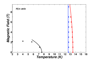
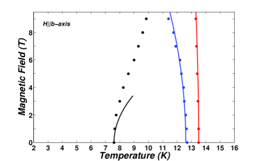
Figure 1: (Color online) Magnetoelectric phase diagrams of MnWO₄ with magnetic fields parallel to the (a) easy and (b) b axes. The solid lines are the calculated transition temperatures and the dots describe the experimental points of Arkenbout et al..AAH06 The calculated phase diagrams were obtained by setting $b=0.095k_{B}K$.

The development of the magnetic order parameters with decreasing temperature has been studied by polarized-neutron diffractions.SH08 Generally, the magnetic moment at site $\tau$ belonging to the unit cell at the lattice point $R$ can be written as

$$\mbox{\boldmath{$m$}}(\mbox{\boldmath{$R$}}+\mbox{\boldmath{$\tau$}}) =m_{x}\cos\left(\mbox{\boldmath{$q$}}\cdot\mbox{\boldmath{$R$}}+\phi_{\tau}\right)\hat{\bf x}$$

$$+m_{b}\sin\left(\mbox{\boldmath{$q$}}\cdot\mbox{\boldmath{$R$}}+\phi_{\tau}\right)\hat{\bf b}.$$ (55)

The cross-sections for polarized-neutron scattering, where the neutrons are polarized parallel and anti-parallel to the scattering vector, are given bySH08

$$I=I{}_{0}\left(m_{x}\pm m_{b}\right)^{2},$$ (56)

with $I_{0}$ being a constant. Using Eqs. (III.1) and (III.1), we see that these cross-sections are proportional to $\left(\left|\sigma^{0}_{x}(\mbox{\boldmath{$q$}}_{IC})\right|\pm\left|\sigma^{0}_{b}(\mbox{\boldmath{$q$}}_{IC})\right|\right)^{2}+\left|\sigma^{0}_{x}(\mbox{\boldmath{$q$}}_{C})\right|^{2}$. Then, from the second of Eqs. (III.1), the magnetic order parameters in the AF2 phase can be written as

$$\left|\sigma^{0}_{x}(\mbox{\boldmath{$q$}}_{IC})\right| =\sqrt{\frac{a\left[\frac{4}{3}\left(T^{(0)}_{N3}-T^{(0)}_{N2}\right)+T^{(0)}_{N2}-T\right]}{8b}},$$

$$\left|\sigma^{0}_{b}(\mbox{\boldmath{$q$}}_{IC})\right| =\sqrt{\frac{a\big{(}T^{(0)}_{N2}-T\big{)}}{8b}}.$$ (57)

Tolédano et al.TP10 assumed that $\left|\sigma^{0}_{x}(\mbox{\boldmath{$q$}}_{IC})\right|$ is fixed below $T^{(0)}_{N2}$. According to the first of Eqs. (IV), such an assumption is valid only for $T^{(0)}_{N2}-T\ll\frac{4}{3}\left(T^{(0)}_{N3}-T^{(0)}_{N2}\right)$. At lower temperatures this assumption is inconsistent with the evolution of the observed integrated intensities reported in Ref. SH08, , which show that both $\left|\sigma^{0}_{x}(\mbox{\boldmath{$q$}}_{IC})\right|$ and $\left|\sigma^{0}_{b}(\mbox{\boldmath{$q$}}_{IC})\right|$ continue to grow below $T_{N2}$, with the ellipticity $p\equiv\frac{m_{b}}{m_{x}}=\frac{\left|\sigma^{0}_{b}(\mbox{\boldmath{$q$}}_{IC})\right|}{\left|\sigma^{0}_{x}(\mbox{\boldmath{$q$}}_{IC})\right|}$ approaching 1 (so that the spiral is almost circular) as the temperature decreases. Therefore, we preferred to use the explicit dependence of $\left|\sigma^{0}_{x}(\mbox{\boldmath{$q$}}_{IC})\right|$ on the temperature. Using Eqs. (IV), the ellipticity below $T_{N2}$ can be written as

$$p=\frac{1}{\sqrt{1+\omega}},$$ (58)

where $\omega\equiv\frac{4\left(T^{0}_{N3}-T^{0}_{N2}\right)}{3\left(T^{0}_{N2}-T\right)}$. Since the difference $T^{0}_{N3}-T^{0}_{N2}\approx 0.8K$ is very small in the case of MnWO₄, the ellipticity rapidly approaches 1 with decreasing temperature in the spiral phase AF2. The small difference $T^{0}_{N3}-T^{0}_{N2}$ for MnWO₄ is a consequence of the small single-ion anisotropy of Mn²⁺ ions. This should be compared with the case of TbMnO₃, for which $T_{N3}\approx 42K$ and $T_{N2}\approx 27K$. In this multiferroic, the ellipticity grows much more slowly with decreasing temperature,YY07 due to the large difference $T^{0}_{N3}-T^{0}_{N2}\approx 15K$, which is in turn a result of the larger single-ion anisotropy of Mn³⁺ ions. In Fig. 2 we sketch the quantities $\left(\left|\sigma^{0}_{x}(\mbox{\boldmath{$q$}}_{IC})\right|\pm\left|\sigma^{0}_{b}(\mbox{\boldmath{$q$}}_{IC})\right|\right)^{2}+\left|\sigma^{0}_{x}(\mbox{\boldmath{$q$}}_{C})\right|^{2}$ from Eqs. (IV) and (34) together with the experimental data points of Ref. SH08, .

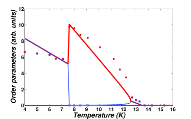
Figure 2: (Color online) The temperature dependence of $\left(\left|\sigma^{0}_{x}(\mbox{\boldmath{$q$}}_{IC})\right|\pm\left|\sigma^{0}_{b}(\mbox{\boldmath{$q$}}_{IC})\right|\right)^{2}+\left|\sigma^{0}_{x}(\mbox{\boldmath{$q$}}_{C})\right|^{2}$. The red (thick) line corresponds to the + sign and the blue (thin) one to the minus sign. The integrated intensities of the polarized-neutron diffraction (scaled by 0.002) from Ref. SH08, are the red dots and the blue empty squares.

The development of the calculated order parameters is in a qualitative agreement with the temperature dependence of the integrated intensities. However, for $T^{(0)}_{N2}-T\gg\frac{4}{3}\left(T^{(0)}_{N3}-T^{(0)}_{N2}\right)$ in the AF2 phase, the quantity $\left(\left|\sigma^{0}_{x}(\mbox{\boldmath{$q$}}_{IC})\right|+\left|\sigma^{0}_{b}(\mbox{\boldmath{$q$}}_{IC})\right|\right)^{2}$ is linear in $T$, in contradiction with the temperature dependence of the integrated intensity, as can be seen in Fig. 2. A possible explanation for this apparent discrepancy is related to fluctuations near the transitions, that are not taken into account by the mean-field Landau theory.Landau&Lifshitz As pointed out in Ref. HAB08, , the transition P$\rightarrow$AF3 belongs to the universality class of the XY model, while the transition AF3$\rightarrow$AF2 belongs to the Ising universality class. Hence we present in Fig. 3 the same quantities as in Fig. 2, but replacing the square roots of Eqs. (IV) and (34) by the critical exponent $\beta=1/3$, roughly appropriate for these two models. As seen from the figure, these revised expressions are in good agreement with the observed integrated intensities. This behavior illustrates the possible importance of fluctuations in MnWO₄. Further consequences of fluctuations near the transitions will be discussed below in the context of the Ginzburg criterion.

Figure 3: (Color online) The temperature dependence of $\left(\left|\sigma^{0}_{x}(\mbox{\boldmath{$q$}}_{IC})\right|\pm\left|\sigma^{0}_{b}(\mbox{\boldmath{$q$}}_{IC})\right|\right)^{2}+\left|\sigma^{0}_{x}(\mbox{\boldmath{$q$}}_{C})\right|^{2}$ with the critical exponent $\beta\approx 1/3$. The red (thick) line corresponds to the + sign and the blue (thin) one to the minus sign. The integrated intensities of the polarized-neutron diffraction (scaled by 0.0014) from Ref. SH08, are the red dots and the blue empty squares.

The magnetoelectric coupling $r$ is determined by fitting Eq. (III.1) to the experimental data of the induced ferroelectric polarization.TK06 The ferroelectric polarization is plotted in Fig. 4(a). The best fit to the experimental data is obtained for the value $\frac{\chi^{0}_{E,b}\left|r\right|}{V_{cell}}=21\mu C/m^{2}$. In addition, the electric susceptibility for $T>T^{(0)}_{N3}$ (in the paraelectric and paramagnetic phase), is experimentally found to be $\chi^{0}_{E,b}=11.3\epsilon_{0}$.TK06 The dimensionless parameter $\gamma$ [see Eq. (22)] is then $\gamma=5.9\cdot 10^{-5}$. This value supports the assumption that the magnetic transitions are almost unaffected by the magnetoelectric coupling. The dielectric constant $\epsilon_{b}=1+\frac{\chi^{0}_{E,b}}{\epsilon_{0}}$ is shown in Fig. 4(b). This result is in good agreement with the experimental measurements of Ref. TK06, . The narrow width of the divergence region is a consequence of the small difference between $\widetilde{T}^{(0)}_{N2}$ and ${T}^{(0)}_{N2}$.

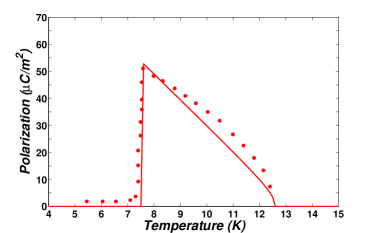
(a)

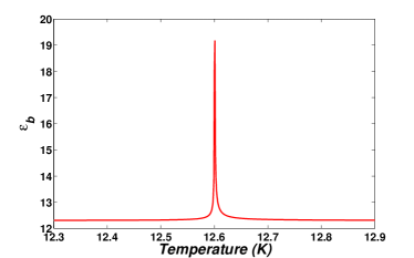
(b)

Figure 4: (Color online) (a) The ferroelectric polarization and (b) the dielectric constant $\epsilon_{b}$. The solid lines are the calculated quantities and the dots are the data points of Taniguchi et al..TK06 The calculated polarization was obtained by setting $\frac{\chi^{0}_{E,b}\left|r\right|}{V_{cell}}=21\mu C/m^{2}$.

Once again, the discrepancy between the linear behavior of the calculated polarization and the observed one may be reconciled by assuming a critical exponent $\beta\approx\frac{1}{3}$ for the magnetic order parameters. The behavior of the calculated polarization in this case is given in Fig. 5.

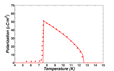
Figure 5: (Color online) The ferroelectric polarization calculated with the critical exponent $\beta\approx\frac{1}{3}$. The solid lines are the calculated quantities and the dots are the experimental points of Taniguchi et al..TK06 The calculated polarization was obtained by setting $\frac{\chi^{0}_{E,b}\left|r\right|}{V_{cell}}=27.5\mu C/m^{2}$.

To examine the effect of Fe doping, we use the relations (51) and (III.3) in the expressions for the transition temperatures and fit the slope to the experimental value according to the $x-T$ phase diagram of Chaudhury et al..CRP09 This procedure yields the values $c_{1}\approx-3.26k_{B}K$, $c_{2}\approx 13.03k_{B}K$ and $c_{3}\approx-1.3$. The anisotropy energy increases with increasing Fe concentration, as expected, since as opposed to the Mn²⁺ ion, the Fe²⁺ ion possesses a non-vanishing angular momentum.HN10

Calculating the different parameters for a small Fe concentration $x$ and repeating the calculations of the $T-H$ phase diagram, we can check the consistency of the above results. The resulting phase diagram for $x=0.035$ is shown in Fig. 6. Except for high fields or low temperatures, the result is in fine agreement with the measurement of Ye et al..YF08 The reentrant ferroelectric phase observed at low temperaturesCRP09 ; CRP09b may be explained by higher order terms in the free energy expansion.

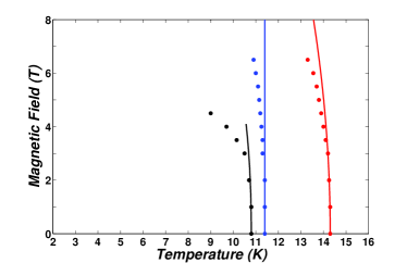
Figure 6: (Color online) Magnetoelectric phase diagram of Mn_0.965Fe_0.035WO₄ with the magnetic field parallel to the easy axis. The solid lines are the calculated transition temperatures and the dots are the experimental points of Ye et al..YF08

The effect of non-magnetic ions on the transition temperatures $T_{N3}(x)$ and $T_{N2}(x)$ is given by Eq. (III.3). These results are drawn in Fig. 7 together with the experimental data of Chaudhury et al.CRP11 of Mn_1-xZn_xWO₄. Similar results have been observed in Mn_1-xMg_xWO₄.ML09 We stress that unlike the case of Fe doping, the results for the transition temperatures $T_{N3}(x)$ and $T_{N2}(x)$ in the case of non-magnetic ions doping do not require additional phenomenological parameters.

As opposed to $T_{N3}(x)$ and $T_{N2}(x)$, the calculated transition temperature $T_{N1}(x)$ does not coincide with the experimentally measured one.CRP11 The discrepancy may be explained by allowing small changes in the exchange couplings $J^{\text{Mn-Mn}}_{i}$ due to spin-lattice coupling (or exchange striction). In other words, if we assume that $J^{\text{Mn-Mn}}_{i}(x)=J^{\text{Mn-Mn}}_{i}(1+\xi_{i}x)$ with $\xi_{i}x\ll 1$, then $T_{N1}(x)$ changes dramatically while $T_{N3}(x)$ and $T_{N2}(x)$ are almost not influenced. The reason for this behavior is that the transition temperature $T_{N1}$ [see Eq. (38)] is much more sensitive to small changes in the exchange couplings than the transition temperatures $T_{N3}$ and $T_{N2}$ [see Eqs. (18) and (25)]. A significant spin-lattice coupling in the multiferroic MnWO₄ has been demonstrated TK08 by the appearance of an incommensurate lattice modulation in the AF3 and AF2 phases, with a lattice propagation vector equal to twice the magnetic propagation vector. In addition, thermal expansion measurements reveal considerable discontinuities in the lattice parameters at the AF2$\rightarrow$AF1 first order phase transition.CRP08b Another indication for a dependence of the Mn-Mn exchange couplings on the non-magnetic dopant concentration is provided by the small change of the incommensurate propagation vector from $\mbox{\boldmath{$q$}}_{IC}=(-0.214,0.5,0.457)$ in MnWO₄ to $\mbox{\boldmath{$q$}}_{IC}=(-0.209,0.5,0.453)$ in Mn_0.85Zn_0.15WO₄.ML09

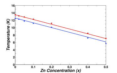
Figure 7: (Color online) Transition temperatures $T_{N3}(x)$ and $T_{N2}(x)$ of Mn_1-xZn_xWO₄. The solid lines are the calculated transition temperatures and the dots are the data points of Chaudhury et al..CRP11

The next step is to compare the above fitted parameters with the parameters calculated directly from the experimental sets of exchange couplings of Ehrenberg et al. and Ye et al.. The calculated exchange couplings of Ref. TC09, yield much higher transition temperatures than the observed ones and thus will not be discussed here. Indeed, The problem of overestimation of exchange interactions by DFT calculations has been indicated by the authors.TC09

The first step is to maximize $\lambda_{+}(\mbox{\boldmath{$q$}})$ [see Eq. (II)] in order to find the incommensurate wave vector $\mbox{\boldmath{$q$}}_{IC}$ and the corresponding eigenvalue $\lambda_{+}(\mbox{\boldmath{$q$}}_{IC})$. The maximization process yields $\mbox{\boldmath{$q$}}_{IC}=(-0.28,0.5,0.44)$ and $\lambda_{+}(\mbox{\boldmath{$q$}}_{IC})=3.82k_{B}K$ for the $J_{1}-J_{9}$ values of Ehrenberg et al.,EH99 while for the $J_{1}-J_{11}$ values of Ye et al.YF11 we find $\mbox{\boldmath{$q$}}_{IC}=(-0.3,0.5,0.49)$ and $\lambda_{+}(\mbox{\boldmath{$q$}}_{IC})=3.85k_{B}K$. These results are in qualitative agreement with the incommensurate wave vector $\mbox{\boldmath{$q$}}_{IC}=(-0.214,\frac{1}{2},0.457)$ observed in experiments. However, the differences are not negligible, suggesting possible errors in the experimental sets of exchange couplings. In addition, the transition temperatures $T^{(0)}_{N3}$ and $T^{(0)}_{N2}$ calculated from Eqs. (18) and (25) with $a_{\text{Mn}}=0.343k_{B}$ [see Eq. (43)] are found to be $T^{(0)}_{N3}=12.79K$, $T^{(0)}_{N2}=10.3K$ for the set of Ehrenberg et al. and $T^{(0)}_{N3}=13.67K$, $T^{(0)}_{N2}=10K$ for the set of Ye et al.. These values slightly differ from the observed transition temperatures, especially the second one. The ratio $\eta=\frac{\lambda_{+}(\mbox{\boldmath{$q$}}_{C})}{\lambda_{+}(\mbox{\boldmath{$q$}}_{IC})}$ is found to be $\eta=0.974$ and $\eta=0.97$ for the sets of Ehrenberg et al. and Ye et al., respectively. Table  2 summarizes the values of $\lambda_{+}(\mbox{\boldmath{$q$}}_{IC})$, $D$ and $\eta$ calculated from the experimental sets of magnetic parameters and those fitted to the experimental transition temperatures.

Table 2: Comparison between the model parameters calculated from the experimental sets of Ref. EH99, and Ref. YF11, and those fitted to the experimental transition temperatures.

Parameter	Ref. EH99,	Ref. YF11,	This work
$\lambda_{+}(\mbox{\boldmath{$q$}}_{IC})(k_{B}K)$	3.82	3.85	4.36-4.45
$D(k_{B}K)$	0.568	0.83	0.27-0.18
$\eta$	0.974	0.97	0.97-0.98

The calculation of the Curie-Weiss temperature reveals a much more serious discrepancy. According to Eq. (44), the Curie-Weiss temperature is $\theta_{x}=-7.6K$, $\theta_{b}=-9.25K$ for the set of Ehrenberg et al. and $\theta_{x}=-23.2K$, $\theta_{b}=-25.65K$ for the set of Ye et al.. These values do not fit the experimental Curie-Weiss temperature $\theta\approx-75K$.AAH06 ; DH69 We suspect that the origin of most of the discrepancies are errors in the set of magnetic couplings. The results suggested by our model may be used as additional constraints in the determination of those couplings. As mentioned before, an additional possible cause for the above discrepancies is related to fluctuations near the transitions, as will be discussed in the next section.

V The Ginzburg criterion

The results of the preceding sections have been obtained within the mean-field approximation. Here we estimate the Ginzburg range, in which fluctuations become important, near the first transition P$\rightarrow$AF3, by two methods. First we compare the mean square fluctuation of the order parameter $\sigma_{x}(\mbox{\boldmath{$q$}}_{IC})$ with the mean-field value, and then we compare the discontinuity in the heat capacity derived from the Landau theory with the divergent heat capacity, originating from the fluctuations at quadratic order.Landau&Lifshitz

Let us denote by $\delta\sigma_{x}(\mbox{\boldmath{$q$}})=\sigma_{x}(\mbox{\boldmath{$q$}})-\langle\sigma_{x}(\mbox{\boldmath{$q$}})\rangle$ the fluctuation of the order parameter in the AF3 phase. The correlation function of these deviations is

$$\langle\delta\sigma_{x}(\mbox{\boldmath{$q$}})\delta\sigma_{x}(\mbox{\boldmath{$q$}}^{\prime})\rangle=\frac{k_{B}T\delta_{\mbox{\boldmath{$q$}}^{\prime},-\mbox{\boldmath{$q$}}}}{4N\left(D+\lambda_{+}(\mbox{\boldmath{$q$}})-aT\right)},$$ (59)

where $N$ is the number of unit cells in the correlation volume. We can find the correlation lengths by expanding $\lambda_{+}(\mbox{\boldmath{$q$}})$ to second order around $\mbox{\boldmath{$q$}}_{IC}$:

$$\lambda_{+}(\mbox{\boldmath{$q$}})\approx\lambda_{+}(\mbox{\boldmath{$q$}}_{IC})+\sum_{i,j}M_{ij}\left(q_{i}-q_{IC,i}\right)\left(q_{j}-q_{IC,j}\right),$$ (60)

with $M_{ij}\equiv\frac{1}{2}\frac{\partial^{2}\lambda_{+}(\mbox{\boldmath{$q$}})}{\partial q_{i}\partial q_{j}}\bigg{|}_{\mbox{\boldmath{$q$}}=\mbox{\boldmath{$q$}}_{IC}}$. Denoting by $\mu_{1}$, $\mu_{2}$ and $\mu_{3}$ the three eigenvalues of the positive matrix $-M_{ij}$, the three correlation lengths are

$$\xi_{i}=\sqrt{\frac{\mu_{i}}{a\left(T^{(0)}_{N3}-T\right)}}.$$ (61)

Substituting $\mbox{\boldmath{$q$}}=\mbox{\boldmath{$q$}}_{IC}$ and $N=\frac{\xi_{1}\xi_{2}\xi_{3}}{V_{cell}}$ in Eq. (59), the condition $\langle\left|\delta\sigma_{x}(\mbox{\boldmath{$q$}}_{IC})\right|^{2}\rangle\ll\left|\sigma^{0}_{x}(\mbox{\boldmath{$q$}}_{IC})\right|^{2}$ for the validity of the mean-field theory readsLandau&Lifshitz

$$\frac{k_{B}T^{(0)}_{N3}}{4a\left(T^{(0)}_{N3}-T\right)}\frac{V_{cell}}{\xi_{1}\xi_{2}\xi_{3}}\ll\frac{a\left(T^{(0)}_{N3}-T\right)}{6b}.$$ (62)

Inserting Eq. (61) into Eq. (62) at the Ginzburg temperature $T_{G}$, we find

$$\left|T_{G}-T^{(0)}_{N3}\right|\approx\frac{9k^{2}_{B}b^{2}V^{2}_{cell}\left(T^{(0)}_{N3}\right)^{2}}{4a\mu_{1}\mu_{2}\mu_{3}}.$$ (63)

Equation (63) estimates the temperature range below $T^{(0)}_{N3}$, in which fluctuations are not negligible.

Let us now estimate the Ginzburg range according to the second method. On the one hand, according to Landau theory, the heat capacity $c=-T\frac{\partial^{2}f}{\partial T^{2}}$ grows discontinuously at the transition P$\rightarrow$AF3:

$$\Delta c_{L}\equiv c_{L}\left(T^{(0)-}_{N3}\right)-c_{L}\left(T^{(0)+}_{N3}\right)=\frac{a^{2}T^{(0)}_{N3}}{6b}.$$ (64)

On the other hand, assuming fluctuations at quadratic order, the singular part of the heat capacity is given by

$$c_{G}=\frac{V_{cell}k_{B}a^{2}T^{2}}{2\left(2\pi\right)^{3}}\int_{BZ}\frac{d^{3}q}{\left(aT-D-\lambda_{+}(\mbox{\boldmath{$q$}})\right)^{2}},$$ (65)

where the integral is over the first Brillouin zone. In the neighborhood of $T^{(0)}_{N3}$, the main contribution to the integral comes from the neighborhood of the incommensurate wave vector $\mbox{\boldmath{$q$}}_{IC}$ in reciprocal space. Thus we can use the expansion (60). Replacing the first Brillouin zone by a sphere, and taking $T\approx T^{(0)}_{N3}$, we can estimate the integral in Eq. (65):

$$c_{G}\approx\frac{k_{B}a^{1.5}T^{2}\left(T-T^{(0)}_{N3}\right)^{-0.5}}{16\pi\sqrt{\mu_{1}\mu_{2}\mu_{3}}}.$$ (66)

Comparing Eqs. (64) and (66) at the Ginzburg temperature $T_{G}$, we findLandau&Lifshitz

$$\left|T_{G}-T^{(0)}_{N3}\right|\approx\left(\frac{6}{16\pi}\right)^{2}\frac{k^{2}_{B}b^{2}V^{2}_{cell}\left(T^{(0)}_{N3}\right)^{2}}{a\mu_{1}\mu_{2}\mu_{3}}.$$ (67)

Calculating the eigenvalues $\mu_{1}$, $\mu_{2}$ and $\mu_{3}$ from the experimental sets of exchange couplings, the Ginzburg temperature is estimated to be $\left|T_{G}-T^{(0)}_{N3}\right|\approx 9.41K$ and $\left|T_{G}-T^{(0)}_{N3}\right|\approx 6.24K$ for the sets of Ehrenberg et al. and Ye et al., respectively, by the first method [see Eq. (63)] while it is $\left|T_{G}-T^{(0)}_{N3}\right|\approx 0.06K$ and $\left|T_{G}-T^{(0)}_{N3}\right|\approx 0.04K$ by the second method [see Eq. (67)]. These values suggest that fluctuations of the order parameters can also contribute to the discrepancies between the experimental data and the mean-field Landau theory results.

VI Summary and Conclusions

We have studied the phase diagram of Mn_1-xM_xWO₄ (M=Fe, Zn, Mg) by a semi-phenomenological Landau theory. The energy has been modelled by a Heisenberg Hamiltonian with a single-ion anisotropy, while the entropy has been expanded in powers of the classical spins. This approach is different from the previous theoretical studies,TP10 ; SVP10 which are purely phenomenological, since it enables to compare different sets of exchange couplings. Although a purely phenomenological approach may capture all the symmetry aspects of the problem and may provide a full mapping of the stable states allowed by the order parameter symmetries,TP10 it does not indicate a clear connection between the free energy coefficients and the microscopic interactions. The advantage of our approach is the simple relation of the free energy coefficients with experimentally derived quantities such as the superexchange couplings and the anisotropy coefficients. For instance, this simple relation allows us to consider the effect of different dopants on the phase diagram, not discussed in Ref. TP10, . We emphasize that our approach does not contradict any symmetry requirement.

We used the superexchange interaction couplings from the inelastic neutron scattering studies of Ehrenberg et al.EH99 and Ye et al..YF11 The results show that both sets yield transition temperatures $T^{(0)}_{N3}$ and $T^{(0)}_{N2}$ that slightly deviate from the experimental temperatures, and significantly underestimate the Curie-Weiss temperature $\left|\theta\right|$. In addition, the calculated incommensurate wave vector $\mbox{\boldmath{$q$}}_{IC}$ has non-negligible deviations from the experimentally observed one. The results presented here can serve as additional constraints on a future determination of the magnetic Hamiltonian parameters. Another possible cause for the discrepancies relates to fluctuations near the transitions. We have demonstrated the possible important contribution of fluctuations in MnWO₄. This issue should be further examined in future experiments.

Beyond that, the model clarifies the effect of different dopants on the phase diagram. The sensitivity of the expression (38) for the transition temperature $T_{N1}(x)$ to small changes of the ratio $\eta\equiv\frac{\lambda_{+}(\mbox{\boldmath{$q$}}_{C})}{\lambda_{+}(\mbox{\boldmath{$q$}}_{IC})}$ reflects the frustrated nature of the multiferroic MnWO₄. The origin of the complex phase diagram lies in the competition between different superexchange interactions. Small changes in the local environment of the Mn²⁺ ions due to a chemical doping cause a significant change in the phase diagram. The sensitivity for the local environment manifests itself by the contrasting behavior of doping with different ions.

Looking to the future, two points should be further examined. Firstly, a new analysis of the inelastic scattering experiments, together with the additional constraints provided in this work, should improve the exchange couplings for the multiferroic MnWO₄. Secondly, the measurement of the critical exponents near the transitions would shed light on the effect of fluctuations. This may contribute to the general understanding of critical phenomena in multiferroics.

References

• (1) D. Khomskii, Physics 2, 20 (2009).
• (2) S.-W. Cheong and M. Mostovoy, Nat. Mater. 6, 13 (2007).
• (3) M. Fiebig, J. Phys. D 38, R123 (2005).
• (4) T. Kimura, Annu. Rev. Mater. Res. 37, 387 (2007).
• (5) T. Kimura, T. Goto, H. Shintani, K. Ishizaka, T. Arima, and Y. Tokura, Nature (London) 426, 55 (2003).
• (6) N. Hur, S. Park, P. A. Sharma, J. S. Ahn, S. Guha, and S.-W. Cheong, Nature (London) 429, 392 (2004).
• (7) G. Lawes, A. B. Harris, T. Kimura, N. Rogado, R. J. Cava, A. Aharony, O. Entin-Wohlman, T. Yildrim, M. Kenzelmann, C. Broholm, and A. P. Ramirez, Phys. Rev. Lett. 95, 087205 (2005).
• (8) T. Kimura, J. C. Lashley, and A. P. Ramirez, Phys. Rev. B 73, 220401(R) (2006).
• (9) Y. Yamasaki, S. Miyasaka, Y. Kaneko, J.-P. He, T. Arima, and Y. Tokura, Phys. Rev. Lett. 96, 207204 (2006).
• (10) S. Picozzi and C. Ederer, J. Phys. Condens. Matter 21, 303201 (2009).
• (11) M. Mostovoy, Phys. Rev. Lett. 96, 067601 (2006).
• (12) A. B. Harris, Phys. Rev. B 76, 054447 (2007).
• (13) A. B. Harris, T. Yildrim, A. Aharony, and O. Entin-Wohlman, Phys. Rev. B 73, 184433 (2006).
• (14) H. Katsura, N. Nagaosa, and A. V. Balatsky, Phys. Rev. Lett. 95, 057205 (2005).
• (15) I. A. Sergienko and E. Dagotto, Phys. Rev. B 73, 094434 (2006).
• (16) G. Lautenschläger, H. Weitzel, T. Vogt, R. Hock, A. Böhm, M. Bonnet, and H. Fuess, Phys. Rev. B 48, 6087 (1993).
• (17) A. H. Arkenbout, T. T. M. Palstra, T. Siegrist, and T. Kimura, Phys. Rev. B 74, 184431 (2006).
• (18) K. Taniguchi, N. Abe, T. Takenobu, Y. Iwasa, and T. Arima, Phys. Rev. Lett. 97, 097203(2006).
• (19) H. Weitzel and H. Langhof, J. Magn. Magn. Mater. 4, 265 (1977).
• (20) R. P. Chaudhury, B. Lorenz, Y. Q. Wang, Y. Y. Sun, and C. W. Chu, New J. Phys. 11, 033036 (2009).
• (21) F. Ye, Y. Ren, J. A. Fernandez-Baca, H. A. Mook, J. W. Lynn, R. P. Chaudhury, Y.-Q. Wang, B. Lorenz, and C. W. Chu, Phys. Rev. B 78, 193101 (2008).
• (22) R. P. Chaudhury, B. Lorenz, Y. Q. Wang, Y. Y. Sun, and C. W. Chu, Phys. Rev. B 77, 104406 (2008).
• (23) Y.-S. Song, J.-H. Chung, J. M. S. Park, and Y.-N. Choi, Phys. Rev. B 79, 224415 (2009).
• (24) R. P. Chaudhury, F. Ye, J. A. Fernandez-Baca, B. Lorenz, Y. Q. Wang, Y. Y. Sun, H. A. Mook, and C. W. Chu, Phys. Rev. B 83, 014401 (2011).
• (25) L. Meddar, M. Josse, P. Deniard, C. La, G. André, F. Damay, V. Petricek, S. Jobic, M.-H. Whangbo, M. Maglione, and C. Payen, Chem. Mater. 21, 5203 (2009).
• (26) H. Ehrenberg, H. Weitzel, H. Fuess, and B. Hennion, J. Phys. Condens. Matter 11, 2649 (1999).
• (27) C. Tian, C. Lee, H. Xiang, Y. Zhang, C. Payen, S. Jobic, and M.-H. Whangbo, Phys. Rev. B 80, 104426 (2009).
• (28) F. Ye, R. S. Fishman, J. A. Fernandez-Baca, A. A. Podlesnyak, G. Ehlers, H. A. Mook, Y. Wang, B. Lorenz, and C. W. Chu, Phys. Rev. B 83, 140401(R) (2011).
• (29) The values of the experimental parameters were adjusted to the definitions of Eq. (1), in which each pair of spins is counted once, and the anisotropy term includes a prefactor $\frac{1}{2}$.
• (30) H. Sagayama, K. Taniguchi, N. Abe, T. Arima, M. Soda, M. Matsuura, and K. Hirota, Phys. Rev. B 77, 220407(R) (2008).
• (31) T. Finger, D. Senff, K. Schmalzl, W. Schmidt, L. P. Regnault, P. Becker, L. Bohatý, and M. Braden, Phys. Rev. B 81, 054430 (2010).
• (32) We note that Eq.(39) has a positive sign since the magnetic moment of electrons is opposite to the spin direction.
• (33) N. W. Ashcroft and N. D. Mermin, Solid State Physics (Saunders, Philadelphia, 1976), Ch. 33.
• (34) H. Dachs, Solid State Commun. 7, 1015 (1969).
• (35) P. Tolédano, B. Mettout, W. Schranz, and G. Krexner, J. Phys. Condens. Matter 22, 065901 (2010).
• (36) Y. Yamasaki, H. Sagayama, T. Goto, M. Matsuura, K. Hirota, T. Arima, and Y. Tokura, Phys. Rev. Lett. 98, 147204 (2007).
• (37) L. D. Landau and E. M. Lifshitz, Statistical Physics (Pergamon, London, 1958), Ch. XIV.
• (38) A. B. Harris, A. Aharony, and O. Entin-Wohlman, J. Phys. Condens. Matter 20, 434202 (2008).
• (39) N. Hollmann, Z. Hu, T. Willers, L. Bohatý, P. Becker, A. Tanaka, H. H. Hsieh, H.-J. Lin, C. T. Chen, and L. H. Tjeng, Phys. Rev. B 82, 184429 (2010).
• (40) R. P. Chaudhury, B. Lorenz, Y. Q. Wang, Y. Y. Sun, C. W. Chu, F. Ye, J. Fernandez-Baca, H. Mook, and J. Lynn, J. Appl. Phys. 105, 07D913 (2009).
• (41) K. Taniguchi, N. Abe, H. Sagayama, S. Ohtani, T. Takenobu, Y. Iwasa, and T. Arima, Phys. Rev. B 77, 064408 (2008).
• (42) R. P. Chaudhury, F. Yen ,C. R. Dela Cruz, B. Lorenz, Y. Q. Wang, Y. Y. Sun, and C. W. Chu, Physica B 403, 1428 (2008).
• (43) V. P. Sakhnenko, N. V. Ter-Oganessian, J. Phys. Condens. Matter 22, 226002 (2010).