A Kernel Multiple Change-point Algorithm via Model Selection
Abstract
We tackle the change-point problem with data belonging to a general set. We build a penalty for choosing the number of change-points in the kernel-based method of Harchaoui and Cappé (2007). This penalty generalizes the one proposed by Lebarbier (2005) for a one-dimensional signal changing only through its mean. We prove a non-asymptotic oracle inequality for the proposed method, thanks to a new concentration result for some function of Hilbert-space valued random variables. Experiments on synthetic and real data illustrate the accuracy of our method, showing that it can detect changes in the whole distribution of data, even when the mean and variance are constant.
Keywords: model selection, kernel methods, change-point detection, concentration inequality
1 Introduction
The change-point problem has been tackled in numerous papers in the statistics and machine learning literature (Brodsky and Darkhovsky, 1993; Carlstein et al., 1994; Tartakovsky et al., 2014; Truong et al., 2019). Given a time series, the goal is to split it into homogeneous segments, in which the marginal distribution of the observations —their mean or their variance, for instance— is constant. When the number of change-points is known, this problem reduces to estimating the change-point locations as precisely as possible; in general, the number of change-points itself must be estimated. This problem arises in a wide range of applications, such as bioinformatics (Picard et al., 2005; Curtis et al., 2012), neuroscience (Park et al., 2015), audio signal processing (Wu and Hsieh, 2006), temporal video segmentation (Koprinska and Carrato, 2001), hacker-attacks detection (Wang et al., 2014), social sciences (Kossinets and Watts, 2006) and econometrics (McCulloh, 2009).
Related work
A large part of the literature on change-point detection deals with observations in or and focuses on detecting changes arising in the mean and/or the variance of the signal (Gijbels et al., 1999; Picard et al., 2005; Arlot and Celisse, 2011; Bertin et al., 2014). To this end, parametric models are often involved to derive change-point detection procedures. For instance, Comte and Rozenholc (2004), Lebarbier (2005), Picard et al. (2011) and Geneus et al. (2014) make a Gaussian assumption, while Frick et al. (2014) and Cleynen and Lebarbier (2014) consider an exponential family.
The challenging problem of detecting abrupt changes in the full distribution of the data has been recently addressed in the nonparametric setting. However, the corresponding procedures suffer several limitations since they are limited to real-valued data or they assume that the number of true change-points is known. For instance, Zou et al. (2014) design a strategy based on empirical cumulative distribution functions that allows to recover an unknown number of change-points by use of BIC, but only applies to -valued data. The strategy of Matteson and James (2014) applies to multivariate data, but it is time-consuming due to an intensive permutation use, and fully justified only in an asymptotic setting when there is a single change-point (Biau et al., 2016). The kernel-based procedure proposed by Harchaoui and Cappé (2007) enables to deal not only with vectorial data but also with structured data in the sense of Gärtner (2008), but it assumes that the number of change-points to recover is known, which reduces its practical interest when no such information is available. Finally, many of these procedures are theoretically grounded only by asymptotic results, which makes their finite-sample performance questionable.
Other attempts have been made to design change-point detection procedures allowing to deal with complex data (that are not necessarily vectors). However, the resulting procedures do not allow to detect more than one or two changes arising in particular features of the distribution. For instance, Chen and Zhang (2015) describe a strategy based on a dissimilarity measure between individuals to compute a graph from which a statistical test allows to detect only one or two change-points. For a graph-valued time series, Wang et al. (2014) design specific scan statistics to test whether one change arises in the connectivity matrix.
Main contributions
We first describe a new efficient multiple change-point detection procedure (KCP) allowing to deal with univariate, multivariate or complex data (DNA sequences or graphs, for instance) as soon as a positive semidefinite kernel can be defined for them. Among several assets, this procedure is nonparametric and does not require to know the true number of change-points in advance. Furthermore, it allows to detect abrupt changes arising in the full distribution of the data by using a characteristic kernel; it can also focus on changes in specific features of the distribution by choosing an appropriate kernel.
Secondly, our procedure (KCP) is theoretically grounded with a finite-sample optimality result, namely an oracle inequality in terms of quadratic risk, stating that its performance is almost the same as that of the best one within the class we consider (Theorem 2). As argued by Lebarbier (2005) for instance, such a guarantee is what we want for a change-point detection procedure. It means that the procedure detects only changes that are “large enough” given the noise level and the amount of data available, which is necessary to avoid having many false positives. A crucial point is that Theorem 2 holds true for any value of the sample size ; in particular it can be smaller than the dimensionality of the data. Note that contrary to previous oracle inequalities in the change-point detection framework, our result requires neither the variance to be constant nor the data to be Gaussian.
Thirdly, we settle a new concentration inequality for the quadratic norm of sums of independent Hilbert-valued vectors with exponential tails, which is a key result to derive our non-asymptotic oracle inequality with a large collection of candidate segmentations. The application domain of our exponential concentration inequality is not limited to change-point detection.
Let us finally mention that since the first version of the present work (Arlot et al., 2012), KCP has been successfully applied on different practical examples. Celisse et al. (2018) illustrate that KCP outperforms state-of-the-art approaches on biological data. Cabrieto et al. (2017) show that KCP with a Gaussian kernel outperforms three non-parametric methods for detecting correlation changes in synthetic multivariate time series, and provide an application to some data from behavioral sciences. Applying KCP to running empirical correlations (Cabrieto et al., 2018b) or to the autocorrelations of a multivariate time series (Cabrieto et al., 2018a) can make it focus on a specific kind of change —in the covariance between coordinates or in the autocorrelation structure of each coordinate, respectively—, as illustrated on synthetic data experiments and two real-world datasets from psychology.
Outline
Motivating examples are first provided in Section 2 to highlight the wide applicability of our procedure to various important settings. A comprehensive description of our kernel change-point detection algorithm (KCP, or Algorithm 1) is provided in Section 3, where we also discuss algorithmic aspects as well as the practical choice of influential parameters (Section 3.3). Section 4 exposes some important ideas underlying KCP and then states the main theoretical results of the paper (Proposition 1 and Theorem 2). Proofs of these main results have been collected in Section 5, while technical details have been deferred to Appendices A and B. The practical performance of the kernel change-point detection algorithm is illustrated by experiments on synthetic data in Section 6 and on real data in Section 7. Section 8 concludes the paper by a short discussion.
Notation.
For any , we denote by the set of integers between and .
2 The change-point problem
Let be some measurable set and a sequence of independent -valued random variables. For any , we denote by the distribution of . The change-point problem can then be summarized as follows: Given , the goal is to find the locations of the abrupt changes along the sequence . Note that the case of dependent time series is often considered in the change-point literature (Lavielle and Moulines, 2000; Bardet and Kammoun, 2008; Bardet et al., 2012; Chang et al., 2014); as a first step, this paper focuses on the independent case for simplicity.
An important example to have in mind is when corresponds to the observation at time of some random process on , and we assume that this process is stationary over , , for some fixed sequence . Then, the change-point problem is equivalent to localizing the change-points , which should be possible as the sample size tends to infinity. Note that we never make such an asymptotic assumption in the paper, where all theoretical results are non-asymptotic.
Let us now detail some motivating examples of the change-point problem.
Example 1
The set is or , and the sequence changes only through its mean. This is the most classical setting, for which numerous methods have been proposed and analyzed in the one-dimensional setting (Comte and Rozenholc, 2004; Zhang and Siegmund, 2007; Boysen et al., 2009; Korostelev and Korosteleva, 2011; Fryzlewicz, 2014) as well as the multi-dimensional case (Picard et al., 2011; Bleakley and Vert, 2011; Hocking et al., 2013; Soh and Chandrasekaran, 2017; Collilieux et al., 2015).
Example 2
The set is or , and the sequence changes only through its mean and/or its variance (or covariance matrix). This setting is rather classical, at least in the one-dimensional case, and several methods have been proposed for it (Andreou and Ghysels, 2002; Picard et al., 2005; Fryzlewicz and Subba Rao, 2014; Cabrieto et al., 2017).
Example 3
The set is or , and no assumption is made on the changes in the sequence . For instance, when data are centered and normalized, as in the audio-track example (Rabiner and Schäfer, 2007), the mean and the variance of the can be constant, and only higher-order moments of are changing. Only a few recent papers deal with (an unknown number of) multiple change-points in a fully nonparametric framework: Zou et al. (2014) for , Matteson and James (2014) for . Note that assuming and adding some further restrictions on the maximal order of the moments for which a change can arise in the sequence , it is nevertheless possible to consider the multivariate sequence , where is a polynomial of degree for , and to use a method made for detecting changes in the mean (Example 1). For instance with -valued data, one can take for every , or equal to the -th Hermite polynomial, as proposed by Lajugie et al. (2014).
Example 4
The set is the -dimensional simplex . For instance, audio and video data are often represented by histogram features (Oliva and Torralba, 2001; Lowe, 2004; Rabiner and Schäfer, 2007), as done in Section 7. In such cases, it is a bad idea to do as if were -valued, since the Euclidean norm on is usually a bad distance measure between histogram data.
Example 5
The set is a set of graphs. For instance, the can represent a social network (Kossinets and Watts, 2006) or a biological network (Curtis et al., 2012) that is changing over time (Chen and Zhang, 2015). Then, detecting meaningful changes in the structure of a time-varying network is a change-point problem. In the case of social networks, this can be used for detecting the rise of an economic crisis (McCulloh, 2009).
Example 6
The set is a set of texts (strings). For instance, text analysis can try to localize possible changes of authorship within a given text (Chen and Zhang, 2015).
Example 7
The set is a subset of , the set of DNA sequences. For instance, an important question in phylogenetics is to find recombination events from the genome of individuals of a given species (Knowles and Kubatko, 2010; Ané, 2011). This can be achieved from a multiple alignment of DNA sequences (Schölkopf et al., 2004) by detecting abrupt changes (change-points) in the phylogenetic tree at each DNA position, that is, by solving a change-point problem.
Example 8
Example 9
The set is an infinite-dimensional functional space. Such functional data arise in various fields (see for instance Ferraty and Vieu, 2006, Chapter 2), and the problem of testing whether there is a change or not in a functional time series has been considered recently (Ferraty and Vieu, 2006; Berkes et al., 2009; Sharipov et al., 2014).
Other kinds of data could be considered, such as counting data (Cleynen and Lebarbier, 2014; Alaya et al., 2015), qualitative descriptors, as well as composite data, that is, data that are mixing several above examples.
The goal of the paper is to propose a change-point algorithm that is (i) general enough to handle all these situations (up to the choice of an appropriate similarity measure on ), (ii) in a non parametric framework, (iii) with an unknown number of change-points, and (iv) that we can analyze theoretically in all these examples simultaneously.
Note also that we want our algorithm to output a set of change-points that are “close to” the true ones, at least when is large enough. But in settings where the signal-to-noise ratio is not large enough to recover all true change-points (for a given ), we do not want to have false positives. This motivates the non-asymptotic analysis of our algorithm that we make in this paper. Since our algorithm relies on a model selection procedure, we prove in Section 4 an oracle inequality, as usually done in non-asymptotic model selection theory.
3 Detecting changes in the distribution with kernels
Our approach for solving the general change-point problem uses positive semidefinite kernels. It can be sketched as follows.
3.1 Kernel change-point algorithm
For any integer , the set of sequences of change-points is defined by
| (1) |
where are the change-points, and are just added for notational convenience. Any is called a segmentation (of ) into segments.
Let be a positive semidefinite kernel, that is, a measurable function such that for any , the matrix is positive semidefinite. Examples of such kernels are given in Section 3.2. Then, we measure the quality of any candidate segmentation with the kernel least-squares criterion introduced by Harchaoui and Cappé (2007):
| (2) |
In particular when and , we recover the usual least-squares criterion
Note that Eq. (6) in Section 4.1 provides an equivalent formula for , which is helpful for understanding its meaning. Given the criterion (2), we cast the choice of as a model selection problem (as thoroughly detailed in Section 4), which leads to Algorithm 1 below, that we now briefly comment on.
| Input: | observations: , |
|---|---|
| kernel: , | |
| constants: and . | |
| Step 1: | , compute (by dynamic programming): |
| and | |
| Step 2: | find: |
| . | |
| Output: | sequence of change-points: . |
-
•
Step 1 of KCP consists in choosing the “best” segmentation with segments, that is, the minimizer of the kernel least-squares criterion over , for every .
- •
-
•
Practical issues (computational complexity and choice of constants ) are discussed in Section 3.3. Let us only emphasize here that KCP is computationally tractable; its most expensive part is the minimization problem of Step 1, which can be done by dynamic programming (see Harchaoui and Cappé, 2007; Celisse et al., 2018). An implementation of KCP in python can be found in the ruptures package Truong et al. (2018).
3.2 Examples of kernels
KCP can be used with various sets (not necessarily vector spaces) as long as a positive semidefinite kernel on is available. An important issue is to design relevant kernels, that are able to capture important features of the data for a given change-point problem, including non-vectorial data —for instance, simplicial data (histograms), texts or graphs (networks), see Section 2. The question of choosing a kernel is discussed in Section 8.2.
Classical kernels can be found in the books by Schölkopf and Smola (2001), Shawe-Taylor and Cristianini (2004) and Schölkopf et al. (2004) for instance. Let us mention a few of them:
-
•
When , defines the linear kernel. When , KCP then coincides with the algorithm proposed by Lebarbier (2005).
-
•
When , defines the Gaussian kernel with bandwidth , which is used in the experiments of Section 6.
-
•
When , defines the Laplace kernel with bandwidth .
-
•
When , defines the exponential kernel with bandwidth . Note that, unlike the Gaussian and Laplace kernels, the exponential kernel is not translation-invariant.
-
•
When , , corresponds to the Hermite kernel, where denotes the -th Hermite function with bandwidth . This kernel is used in Section 6.
- •
Note that more generally, Sejdinovic et al. (2013) proved that positive semidefinite kernels can be defined on any set for which a semimetric of negative type is used to measure closeness between points. The so-called energy distance between probability measures is an example (Matteson and James, 2014). In addition, specific kernels have been designed for various kinds of structured data, including all the examples of Section 2 (Cuturi et al., 2005; Shervashidze, 2012; Rakotomamonjy and Canu, 2005; Vedaldi and Zisserman, 2012). Kernels can also be built from convolutional neural networks, with successful applications in computer vision (Mairal et al., 2014; Paulin et al., 2017).
Let us finally remark that KCP can also be used when is not a positive semidefinite kernel; its computational complexity remains unchanged, but we might loose the theoretical guarantees of Section 4.
3.3 Practical issues
Computational complexity.
The discrete optimization problem at Step 1 of KCP is apparently hard to solve since, for each , there are segmentations of into segments. Fortunately, as shown by Harchaoui and Cappé (2007), this optimization problem can be solved efficiently by dynamic programming. In the special case of a linear kernel, we recover the classical dynamic programming algorithm for detecting changes in mean (Fisher, 1958; Auger and Lawrence, 1989; Kay, 1993).
Denoting by the cost of computing for some given , the computational cost of a naive implementation of Step 1 —computing each coefficient of the cost matrix independently— then is in time and in space. The computational complexity can actually be in time and in space as soon as one either uses the summed area table or integral image technique as in (Potapov et al., 2014) or optimizes the interplay of the dynamic programming recursions and cost matrix computations (Celisse et al., 2018). For given constants and , Step 2 is straightforward since it consists in a minimization problem among terms already stored in memory. Therefore, the overall complexity of KCP is at most in time and in space.
Setting the constants .
At Step 2 of KCP, two constants appear in the penalty term. Theoretical guarantees (Theorem 2 in Section 4) suggest to take large enough, but the lower bound on in Theorem 2 is pessimistic, and the optimal value of certainly depends on unknown features of the data such as their “variance”, as discussed after Theorem 2. In practice the constants must be chosen from data. To do so, we propose a fully data-driven method, based upon the “slope heuristics” (Baudry et al., 2012), that is explained in Section 6.2. Another way of choosing is described in supplementary material (Section B.3).
Setting the constant .
KCP requires to specify the maximal dimension of the segmentations considered, a choice that has three main consequences. First, the computational complexity of KCP is affine in , as discussed above. Second, if is too small —smaller than the number of true change-points that can be detected—, the segmentation provided by the algorithm will necessarily be too coarse. Third, when the slope heuristics is used for choosing , taking larger than the true number of change-points might not be sufficient: better values for can be obtained by taking larger, up to . From our experiments, it seems that is large enough to provide good results.
3.4 Related change-point algorithms
In addition to the references given in the Introduction, let us mention a few change-point algorithms to which KCP is more closely related.
First, some two-sample (or homogeneity) tests based on kernels have been suggested. They tackle a simpler problem than the general change-point problem described in Section 2. Among them, Gretton et al. (2012a) proposed a two-sample test based on a U-statistic of order two, called the maximum mean discrepancy (MMD). A related family of two-sample tests, called -tests, has been proposed by Zaremba et al. (2013); -tests have also been used by Li et al. (2015, 2019) for localizing a single change-point. Harchaoui et al. (2008) proposed a studentized kernel-based test statistic for testing homogeneity. Resampling methods —(block) bootstrap and permutations— have also been proposed for choosing the threshold of several kernel two-sample tests (Fromont et al., 2012; Chwialkowski et al., 2014; Sharipov et al., 2014).
Second, Harchaoui and Cappé (2007) proposed a kernel change-point algorithm when the true number of segments is known, which corresponds to Step 1 of KCP. The present paper proposes a data-driven choice of for which theoretical guarantees are proved.
Third, when and , is the usual least-squares risk and Step 2 of KCP is similar to the penalization procedures proposed by Comte and Rozenholc (2004) and Lebarbier (2005) for detecting changes in the mean of a one-dimensional signal. We refer readers familiar with model selection techniques to Section 4.1 for an equivalent formulation of KCP —in more abstract terms— that clearly emphasizes the links between KCP and these penalization procedures.
4 Theoretical analysis
We now provide theoretical guarantees for KCP. We start by reformulating it in an abstract way, which enlightens how it works.
4.1 Abstract formulation of KCP
Let denote the reproducing kernel Hilbert space (RKHS) associated with the positive semidefinite kernel . The canonical feature map is then defined by for every . A detailed presentation of positive semidefinite kernels and related notions can be found in several books (Schölkopf and Smola, 2001; Cucker and Zhou, 2007; Steinwart and Christmann, 2008).
Let us define for every , , the set of segmentations —see Eq. (1)—, and for every ,
| (3) |
which is a linear subspace of . We also define on the canonical scalar product by for , and we denote by the corresponding norm. Then, for any ,
| (4) |
is the orthogonal projection of onto , and satisfies
| (5) |
The proof of this statement has been deferred to Appendix A.1.
Following Harchaoui and Cappé (2007), the empirical risk defined by Eq. (2) can be rewritten as
| (6) |
as proved in Appendix A.1.
For each , Step 1 of KCP consists in finding a segmentation in segments such that
which is the “kernelized” version of the classical least-squares change-point algorithm (Lebarbier, 2005). Since the penalized criterion of Step 2 is similar to that of Comte and Rozenholc (2004) and Lebarbier (2005), we can see KCP as a “kernelization” of these penalized least-squares change-point procedures.
Let us emphasize that building a theoretically-grounded penalty for such a kernel least-squares change-point algorithm is not straightforward. For instance, we cannot apply the model selection results by Birgé and Massart (2001) that were used by Comte and Rozenholc (2004) and Lebarbier (2005). Indeed, a Gaussian homoscedastic assumption is not realistic for general Hilbert-valued data, and we have to consider possibly heteroscedastic data for which we assume only that is bounded in —see Assumption (Db) in Section 4.3. Note that unbounded data can satisfy Assumption (Db), for instance by choosing a bounded kernel such as the Gaussian or Laplace ones. In addition, dealing with Hilbert-valued random variables instead of (multivariate) real variables requires a new concentration inequality, see Proposition 1 in Section 4.4.
4.2 Intuitive analysis
Section 4.1 shows that KCP can be seen as a kernelization of change-point algorithms focusing on changes of the mean of the signal (Lebarbier, 2005, for instance). Therefore, KCP is looking for changes in the “mean” of , provided that such a notion can be defined.
If is separable and , we can define the (Bochner) mean of (Ledoux and Talagrand, 1991), also called the mean element of , by
| (7) |
Then, we can write
The variables are independent and centered —that is, , . So, we can understand as the least-squares estimator over of .
An interesting case is when is a characteristic kernel (Fukumizu et al., 2008), or equivalently, when is probability-determining (Fukumizu et al., 2004a, b). Then any change in the distribution induces a change in the mean element . In such settings, we can expect KCP to be able to detect any change in the distribution , at least asymptotically. For instance the Gaussian kernel is characteristic (Fukumizu et al., 2004b, Theorem 4), and general sufficient conditions for to be characteristic are known (Sriperumbudur et al., 2010, 2011).
Note that Sharipov et al. (2014) suggest to use as a “kernel” within a two-sample test, in order to look for any change of the distribution of real-valued data (Example 3). This idea is similar to our proposal of using KCP with a characteristic kernel for tackling Example 3, even if we do not advise to take within KCP. Indeed, when , as soon as the are all different so that KCP becomes useless. This illustrates that using a kernel which is not symmetric positive definite should be done cautiously.
4.3 Notation and assumptions
Throughout the paper, we assume that is separable, which is kind of a minimal assumption for two reasons: it allows to define the mean element —see Eq. (7)—, and most reasonable examples satisfy this requirement (Dieuleveut and Bach, 2014, p. 4). Let us further assume
| (Db) |
For every , we also define the “variance” of by
| (8) |
where is an independent copy of , and . Let us make a few remarks.
-
•
If (Db) holds true, then the mean element exists since , the variances are finite and smaller than .
-
•
If (Db) holds true, then admits a covariance operator that is trace-class and .
- •
-
•
Let us consider the case of the linear kernel on . If , then, where is the covariance matrix of . In addition, (Db) holds true if and only if a.s. for all .
4.4 Concentration inequality for some quadratic form of Hilbert-valued random variables
Our main theoretical result, stated in Section 4.5, relies on two concentration inequalities for some linear and quadratic functionals of Hilbert-valued vectors. Here we state the concentration result that we prove for the quadratic term, which is significantly different from existing results and can be of independent interest.
Proposition 1 (Concentration of the quadratic term)
4.5 Oracle inequality for KCP
Similarly to the results of Comte and Rozenholc (2004) and Lebarbier (2005) in the one-dimensional case, we state below a non-asymptotic oracle inequality for KCP. First, we define the quadratic risk of any as an estimator of by
Theorem 2
We consider the framework and notation introduced in Sections 2–4. Let be some constant. Assume that (Db) holds true and that is some penalty function satisfying
| (9) |
Then, some numerical constant exists such that the following holds: if , for every , an event of probability at least exists on which, for every
| (10) |
we have
| (11) |
Theorem 2 is proved in Section 5.5. In addition, Section 5.1 provides some insight about the construction of the penalty suggested by Eq. (9). In a few words, the idea is to take a penalty such that the empirical criterion in Eq. (10) mimics (approximately) the oracle criterion . At least, the penalty must be large enough so that holds true simultaneously for all (up to technical details, see Section 5).
Theorem 2 applies to the segmentation provided by KCP when . Theorem 2 shows that estimates well the “mean” of the transformed time series . Such a non-asymptotic oracle inequality is the usual way to theoretically validate a model selection procedure (Birgé and Massart, 2001, for instance). It is therefore a natural way to theoretically validate any change-point detection procedure based on model selection. As argued by Lebarbier (2005) for instance, proving such a non-asymptotic result is necessary for taking into account situations where some changes are too small to be detected —they are “below the noise level”. By defining the performance of as the quadratic risk of as an estimator of , a non-asymptotic oracle inequality such as Eq. (11) is the natural way to prove that KCP works well for finite sample size and for a set that can have a large dimensionality (possibly much larger than the sample size ). The consistency of KCP for estimating the change-point locations, which is outside the scope of this paper, is discussed in Section 8.1.
The constant in front of the first term in Eq. (11) has no special meaning, and could be replaced by any quantity strictly larger than , at the price of enlarging and .
The value suggested by Theorem 2 for the constants within KCP should not be used in practice because it is likely to lead to a conservative choice for two reasons. First, the minimal value for the constant suggested by the proof of Theorem 2 depends on the numerical constants appearing in the deviation bounds of Propositions 1 and 3, which probably are not optimal. Second, the constant in the penalty is probably pessimistic in several frameworks. For instance with the linear kernel and Gaussian data belonging to , (Db) is not satisfied, but other similar oracle inequalities have been proved with replaced by the residual variance (Lebarbier, 2005). In practice, as we do in the experiments of Section 6, we recommend to use a data-driven value for the leading constant in the penalty, as explained in Section 3.3.
Theorem 2 also applies to KCP with simplified penalty shapes. Indeed, for any ,
so that Theorem 2 applies to the penalty —similar to the one of Lebarbier (2005)— as soon as . A BIC-type penalty is also covered by Theorem 2 provided that and , even if we do not recommend to use it given our experiments —see Section 6.3.
A nice feature of Theorem 2 is that it holds under mild assumptions: we only need the data to be independent and to have (Db) satisfied. As noticed in Section 4.3, (Db) holds true for translation-invariant kernel such as the Gaussian and Laplace kernels. Compared to previous results (Comte and Rozenholc, 2004; Lebarbier, 2005), we do not need the data to be Gaussian or homoscedastic. Furthermore, the independence assumption can certainly be relaxed: to do so, it would be sufficient to prove concentration inequalities similar to Propositions 1 and 3 for some dependent .
In the particular setting where and is the linear kernel , Theorem 2 provides an oracle inequality similar to the one proved by Lebarbier (2005) for Gaussian and homoscedastic real-valued data. The price to pay for extending this result to heteroscedastic Hilbert-valued data is rather mild: we only assume (Db) and replace the residual variance by .
Apart from the results already mentioned, a few oracle inequalities have been proved for change-point procedures, for real-valued data with a multiplicative penalty (Baraud et al., 2009), for discrete data (Akakpo, 2011), for counting data with a total-variation penalty (Alaya et al., 2015), for counting data with a penalized maximum-likelihood procedure (Cleynen and Lebarbier, 2014) and for data distributed according to an exponential family (Cleynen and Lebarbier, 2017). Among these oracle inequalities, only the result by Akakpo (2011) is more precise than Theorem 2 (there is no factor compared to the oracle loss), at the price of using a smaller (dyadic) collection of possible segmentations, hence a worse oracle performance in general.
5 Main proofs
5.1 Outline of the proof of Theorem 2
As usual for proving an oracle inequality (see Arlot, 2014, Section 2.2), we remark that by Eq. (10), for every ,
Therefore,
| (12) | |||
| (13) |
The idea of the proof is that if we had for every , we would get an oracle inequality similar to Eq. (11). What remains to obtain is a deterministic upper bound on the ideal penalty that holds true simultaneously for all on a large probability event. To this aim, our approach is to compute and to show that concentrates around its expectation for every (Sections 5.2–5.4). Then we use a union bound as detailed in Section 5.5. A similar strategy has been used for instance by Comte and Rozenholc (2004) and Lebarbier (2005) in the specific context of change-point detection.
Note that we prove below a slightly weaker result than , which is nevertheless sufficient to obtain Eq. (11). Remark also that Eq. (12) would be true if the constant in the definition (13) of was replaced by any quantity independent from ; the reasons for this specific choice appear in the computations below.
5.2 Computation of the ideal penalty
5.3 Concentration of the linear term
We prove in Section A.2 the following concentration inequality for the linear term in Eq. (14), mostly by applying Bernstein’s inequality.
Proposition 3 (Concentration of the linear term)
If (Db) holds true, then for every , with probability at least ,
| (15) |
5.4 Dealing with the quadratic term
We now focus on the quadratic term in the right-hand side of Eq. (14).
5.4.1 Preliminary computations
We start by providing a useful closed-form formula for and by computing its expectation. First, a straightforward consequence of Eq. (5) is that
| (16) | ||||
| (17) |
Second, we remark that for every ,
| (18) |
5.4.2 Concentration: proof of Proposition 1
This proof is inspired from that of a concentration inequality by Sauvé (2009) in the context of regression with real-valued non-Gaussian noise. Let us define
by Eq. (16). Since the real random variables are independent, we get a concentration inequality for their sum via Bernstein’s inequality (Theorem B.6) as long as satisfies some moment conditions. The rest of the proof consists in showing such moment bounds by using Pinelis-Sakhanenko’s deviation inequality (Proposition B.7).
First, note that (Db) implies that almost surely for every by Lemma A.5, hence a.s. for every . Then for every and ,
| (20) |
Second, since almost surely and for every , we get that for every and ,
Hence, the assumptions of Pinelis-Sakhanenko’s deviation inequality (Pinelis and Sakhanenko, 1986) —which is recalled by Proposition B.7— are satisfied with and , and we get that for every
Together with Eq. (20), we obtain that
| (21) |
since for every ,
Finally summing Eq. (21) over , it comes
Then, condition (B.33) of Bernstein’s inequality holds true with
Therefore, Bernstein’s inequality (Massart, 2007, Proposition 2.9) —which is recalled by Proposition B.6— shows that for every , with probability at least ,
5.4.3 Why do we need a new concentration inequality?
We now review previous concentration results for quantities such as or , showing that they are not sufficient for our needs, hence requiring a new result such as Proposition 1.
First, when is a Gaussian isotropic vector, is a chi-square random variable for which concentration tools have been developed. Such results have been used by Birgé and Massart (2001) and by Lebarbier (2005) for instance. They cannot be applied here since cannot be assumed Gaussian, and the do not necessarily have the same variance.
Second, Eq. (17) shows that is a U-statistic of order 2. Some tight exponential concentration inequalities exist for such quantities when (Houdré and Reynaud-Bouret, 2003) and when belongs to a general measurable set (Giné and Nickl, 2016, Theorem 3.4.8). In both results, a term of order appears in the deviations, which is too large because the proof of Theorem 2 relies on Proposition 1 with : we really need a smaller deviation term, as in Proposition 1 where it is proportional to .
Third, since
Talagrand’s inequality (Boucheron et al., 2013, Corollary 12.12) provides a concentration inequality for around its expectation. More precisely, we can get the following result, which is proved in supplementary material (Section B.2).
Proposition 4
If (Db) holds true, then for every with probability at least ,
| (22) |
Therefore, in order to get a concentration inequality for , we have to square Eq. (22) and we necessarily get a deviation term of order . As with the U-statistics approach, this is too large for our needs.
Fourth, given Eq. (16), it is also natural to think of Pinelis-Sakhanenko’s inequality (Pinelis and Sakhanenko, 1986), but this result alone is not precise enough because it is a deviation inequality, and not a concentration inequality. It is nevertheless a key ingredient in our proof of Proposition 1.
5.5 Oracle inequality: proof of Theorem 2
Upper bound on for every . First, by Eq. (14) for every ,
| (23) |
In other words, is the sum of two terms, for which Propositions 1 and 3 provide concentration inequalities.
On the one hand, by Proposition 1 under (Db), for every and , with probability at least we have
| (24) | ||||
| (25) |
since
by Eq. (19). On the other hand, by Proposition 3 under (Db), for every and , with probability at least we have
| (26) |
For every and , let be the event on which Eq. (25) and (26) hold true. A union bound shows that . Furthermore, combining Eq. (23), (25) and (26) shows that on , for every ,
| (27) |
using that by definition of the orthogonal projection , and
| (28) |
Union bound over the models and conclusion. Let be fixed and let us define the event where for every ,
Then, since
for every , a union bound shows that
In addition, on , for every , since Eq. (27) and (28) hold true with , taking , we get that
Let us define
and assume that . Then, using Eq. (9), we have
Therefore, by Eq. (12), on , for every ,
hence
since for every . Multiplying both sides by , we get that if , on ,
Let us finally define
so that
Then, we get that if , on ,
and the result follows.
6 Experiments on synthetic data
This section reports the results of some experiments on synthetic data that illustrate the performance of KCP.
6.1 Data-generation process
Three scenarios are considered: real-valued data with a changing (mean,variance), real-valued data with constant mean and variance, and histogram-valued data as in Example 4.
In the three scenarios, the sample size is and the true segmentation is made of segments, with change-points , , , , , , , , , (see Figure 1). For each sample, we choose randomly the distribution of the within each segment of as detailed below; note that we always make sure that the distribution of does change at each change-point .
For each scenario, we generate independent samples, from which we estimate all quantities that are reported in Section 6.3.
Scenario 1: Real-valued data with changing (mean, variance).
The distribution of is randomly picked out from: (Binomial), (Negative-Binomial), (Hypergeometric), (Gaussian), (Gamma), (Weibull) and (Pareto). Note that the pair (mean, variance) in each segment changes from that of its neighbors. Table B.1 summarizes its values.
The distribution within segment is given by the realization of a random variable , each integer representing one of the 7 possible distributions. The variables are generated as follows: is uniformly chosen among , and for every , given , is uniformly chosen among . Figure 1a shows one sample generated according to this scenario.

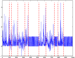

Scenario 2: Real-valued data with constant mean and variance.
The distribution of is randomly chosen among (1) (Bernoulli), (2) (Gaussian) and (3) (Exponential). These three distributions have a mean and a variance .
The distribution within segment is given by the realization of a random variable , similarly to what is done in Scenario 1 (replacing by ). Figure 1b shows one sample generated according to this scenario.
Scenario 3: Histogram-valued data.
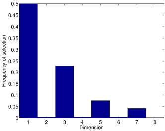
The observations belong to the -dimensional simplex with (Example 4), that is, with . For each , we randomly generate parameter values independently with uniform distribution over with . Then, within the -th segment of , follows a Dirichlet distribution with parameter . Figure 1c displays the first three coordinates of one sample generated according to this scenario.
6.2 Parameters of KCP
For each sample, we apply our kernel change-point procedure (KCP, that is, Algorithm 1) with the following choices for its parameters. We always take .
For the first two scenarios, we consider three kernels:
-
(i)
The linear kernel .
-
(ii)
The Hermite kernel given by defined in Section 3.2. In Scenario 1, . In Scenario 2, .
-
(iii)
The Gaussian kernel defined in Section 3.2. In Scenario 1, . In Scenario 2, .
For Scenario 3, we consider the kernel defined in Section 3.2, and the Gaussian kernel with .
In each scenario several candidate values have been explored for the bandwidth parameters of the above kernels. We have selected the ones with the most representative results.
For choosing the constants arising from Step 2 of KCP, we use the “slope heuristics” method, and more precisely a variant proposed by Lebarbier (2002, Section 4.3.2) for the calibration of two constants for change-point detection. We first perform a linear regression of against and for . Then, denoting by the coefficients obtained, we define for , with . The slope heuristics has been justified theoretically in various settings (for instance by Arlot and Massart, 2009, for regressograms), and is supported by numerous experiments (Baudry et al., 2012), including for change-point detection (Lebarbier, 2002, 2005). A partial theoretical justification has been obtained recently for change-point detection (Sorba, 2017). The intuition behind the slope heuristics is that the optimal amount of penalization needed for avoiding to overfit with is (approximately) proportional to the minimal penalty:
for some constant , equal to in several settings. The linear regression step described above corresponds to estimating the minimal penalty:
Then, multiplying it by leads to an estimation of the optimal penalty. In our experiments, we considered several values of . Remarkably, the performance of the procedure is not too sensitive to the value of provided . We only report the results for because it corresponds to the classical advice when using the slope heuristics, and it is among the best choices for according to our experiments.
6.3 Results
We now summarize the results of our experiments.
Distance between segmentations.
In order to assess the quality of the segmentation as an estimator of the true segmentation , we consider two measures of distance between segmentations. For any , we define the Hausdorff distance between and by
and the Frobenius distance between and (see Lajugie et al., 2014) by
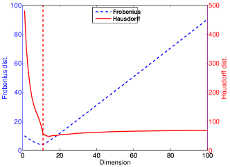
Note that the projection matrix onto when , that is, for the linear kernel on . The Hausdorff distance is probably more classical in the change-point literature, but Figure 2a shows that the Frobenius distance is more informative for comparing . Indeed, when is already a bit larger than , adding false change-points makes the segmentation worse without increasing much ; on the contrary, readily takes into account these additional false change-points.
Illustration of KCP.
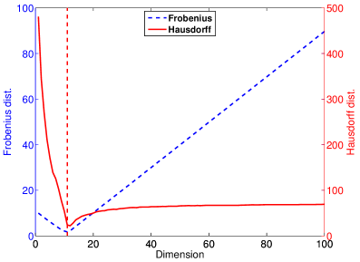
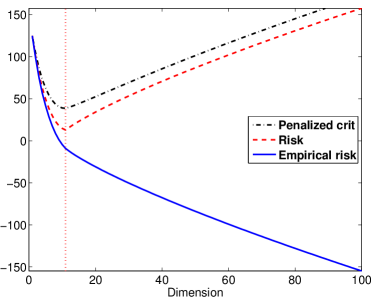

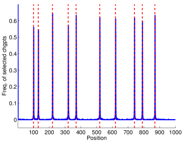
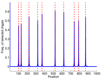
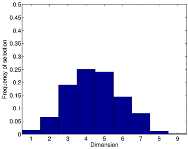
Figure 2 illustrates the typical behaviour of KCP when is well-suited to the change-point problem we consider. It summarizes results obtained in Scenario 1 with the Gaussian kernel.
Figure 2a shows the expected distance between the true segmentation and the segmentations produced at Step 1 of KCP. As expected, the distance is clearly minimal at , for both Hausdorff and Frobenius distances. Note that for each individual sample, behaves exactly as the expectation shown on Figure 2a, up to minor fluctuations. Moreover, the minimal value of the distance is small enough to suggest that is indeed close to . For instance, , with a error bar smaller than . The closeness between and when can also be visualized on Figure B.9c in the supplementary material.
As a comparison, when in the same setting, is much further from since , and a permutation test shows that the difference is significant, with a p-value smaller than . See also Figures B.7 and B.9a in the supplementary material.
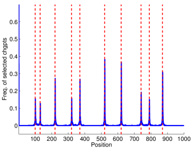
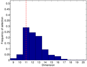
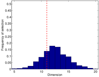
Step 2 of KCP is illustrated by Figures 2b and 2c. The expectation of the penalized criterion is minimal at (as well as for the risk of ), and takes significantly larger values when (Figure 2b). As a result, KCP often selects a number of change-points close to its true value (Figure 2c). Overall, this suggests that the model selection procedure used at Step 2 of KCP works fairly well.
The overall performance of KCP as a change-point detection procedure is illustrated by Figure 2d. Each true change-point has a probability larger than to be recovered exactly by . If one groups the positions by blocks of six elements , , the frequency of detection of a change-point by in each block containing a true change-point is between and . Importantly, such figures are obtained without overestimating much the number of change-points, according to Figure 2c. Figures B.10a and B.10b in the supplementary material show that more standard change-point detection algorithms —that is, KCP with or — have a slightly worse performance.
Comparison of three kernels in Scenario 2.
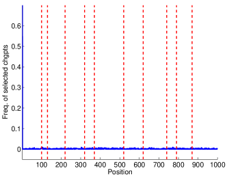
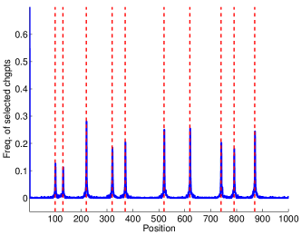
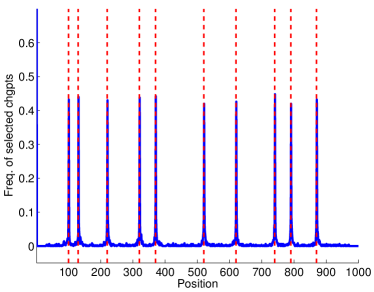
Scenario 2 proposes a more challenging change-point problem with real-valued data: the distribution of the changes while the mean and the variance remain constant. The performance of KCP with three kernels —, and — is shown on Figure 3.
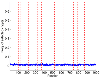
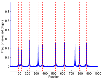
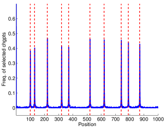

The linear kernel corresponds to the classical least-squares change-point algorithm (Lebarbier, 2005), which is designed to detect changes in the mean, hence it should fail in Scenario 2. KCP with the Hermite kernel is a natural “hand-made” extension of this classical approach, since it corresponds to applying the least-squares change-point algorithm to the feature vectors . By construction, it should be able to detect changes in the first five moments on the . On the contrary, taking the Gaussian kernel fully relies on the versatility of KCP, which makes possible to consider (virtually) infinite-dimensional feature vectors . Since is characteristic, it should be able to detect any change in the distribution of the .
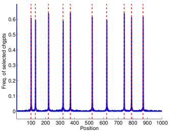
In order to compare these three kernels within KCP, let us first assume that the number of change-points is known, hence we can estimate with , where is the true number of segments. Then, Figures 3a, 3b and 3c show that , and behave as expected: seems to put the change-points of uniformly at random over , while and are able to localize the true change-points with a rather large probability of success. The Gaussian kernel here shows a significantly better detection power, compared to : the frequency of exact detection of the true change-points is between and with , and between and with . The same holds when considering blocks of size : then detects the change-points with probability to , while exhibits probabilities between and .
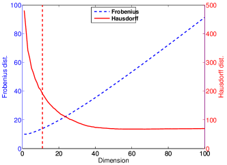
Figures 3d, 3e and 3f show that a similar comparison between , , and holds over the whole set of segmentations provided by Step 1 of KCP. With the linear kernel (Figure 3d), the Frobenius distance between and is almost minimal for , which suggests that is not far from random guessing for all . The shape of the Hausdorff distance —first decreasing fastly, then almost constant— also supports this interpretation: A small number of purely random guesses do lead to a fast decrease of ; and for large dimensions, adding a new random guess does not move away from if already contains all the worst possible candidate change-points (which are the furthest from the true change-points). The Hermite kernel does much better according to Figure 3e: the Frobenius distance from to is minimal for close to , and the minimal expected distance, (with confidence ), is much smaller than when (in which case ); this difference is significant (a permutation test yields a p-value smaller than ). Nevertheless, we still obtain slightly better performance for with , for which the minimal distance to is achieved at , with a minimal expected value equal to (the difference between and is not statistically significant). The Hausdorff distance suggests that both and lead to include false change-points among true ones as long as . However, the smaller Frobenius distance achieved by at (rather than for ) indicates that the corresponding change-points are closer to the true ones than those provided by (which include more false positives).
When is chosen by KCP, clearly leads to the best performance in terms of recovering the exact change-points compared to and , as illustrated by Figures B.11a, B.11b and B.11c in the supplementary material.
Overall, the best performance for KCP in Scenario 2 is clearly obtained with , while completely fails and yields a decent but suboptimal procedure.
We can notice that other settings can lead to different behaviours. For instance, in Scenario 1, according to Figure B.10a in the supplementary material, can detect fairly well the true change-points —as expected since the mean (almost) always changes in this scenario, see Table B.1 in the supplementary material—, but this is at the price of a strong overestimation of the number of change-points (Figure B.8a). In the same setting, provides fairly good results (Figure B.10b), while remains the best choice (Figure 2d).
Since is a characteristic kernel, these results suggest that KCP with a characteristic kernel might be more versatile than classical least-squares change-point algorithms and their extensions. A more detailed simulation experiment would nevertheless be needed to confirm this hypothesis. We also refer to Section 8.2 for a discussion on the choice of for a given change-point problem.
Structured data.
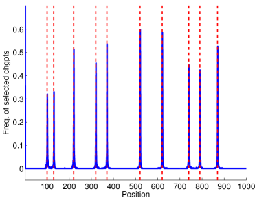
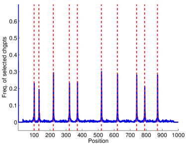
Figure 4 illustrates the performance of KCP on some histogram-valued data (Scenario 3).
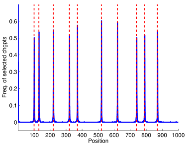
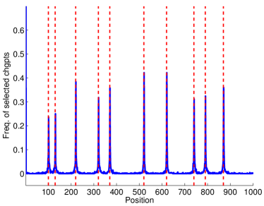
Since a -dimensional histogram is also an element of , we can analyze such data either with a kernel taking into account the histogram structure (such as ) or with a usual kernel on (such as or ; here, we consider , which seems more reliable according to our experiments in Scenarios 1 and 2). Assuming that the number of change-points is known, taking yields quite good results according to Figure 4a, at least in comparison with (Figure 4b). Similar results hold with a fully data-driven number of change-points, as shown by Figures B.13a and B.13b in the supplementary material. Hence, choosing a kernel such as , which takes into account the histogram structure of the , can improve much the change-point detection performance, compared to taking a kernel such as , which ignores the structure of the .
Let us emphasize that Scenario 3 is quite challenging —changes are hard to distinguish on Figure 1c—, which has been chosen on purpose. Preliminary experiments have been done with larger values of —which makes the change-point problem easier, see Section 6.1—, leading to an almost perfect localization of all change-points by KCP with .
Comparison to AIC/BIC-type penalty.
Figures B.14 and B.15 in the supplementary material show the results of KCP with a linear penalty —that is, of the form , — in step 2, similarly to AIC (which would correspond to ) and BIC (for which ). Since is unknown, we use the slope heuristics for choosing from data, as explained in Section 6.2. The performance is comparable to the one of KCP, except that a linear penalty leads to overfitting —by detecting too many change-points (including false positives)— with a large probability in Scenarios 1 and 2 (compare Figures B.14a and B.8c for Scenario 1, and Figures B.14b and B.12c for Scenario 2). Therefore, a linear penalty seems less reliable than the refined shape proposed in the definition of KCP, so we do not recommend to use a linear penalty in practice.
Comparison to the E-divise procedure (ED).
We finally consider the E-divisive procedure (ED) designed by Matteson and James (2014), focusing on Scenarios 1–2 since this procedure is made for only. We use the e.divisive function from the R-package ecp described by James and Matteson (2015), with recommended parameters (significance level to test any new change-point), , and permutations. Detailed results are shown on Figures B.16, B.17 and B.18 in the supplementary material. In both scenarios, ED provides much more conservative results —that is, it strongly underestimates the number of change-points— compared to KCP with . This drawback of ED is particularly clear in Scenario 2 (more difficult) from the comparison of Figures B.12c and B.16b. As a result, ED’s detection power is much smaller than the one of KCP, with detection frequencies 2 to 5 times lower for ED in Scenario 2 (see Figures B.11c and B.17b). The performance of ED improves when is given to the algorithm, but KCP remains significantly better than ED in terms of detection power (see Figures 3c and B.18b, for instance). Overall, KCP with clearly outperforms ED in Scenarios 1–2, which can be explained by at least two reasons: (i) ED uses a different similarity measures than ours; (ii) ED relies on a greedy strategy, in which is obtained from by adding one change-point, so that any mistake at the beginning of the process impacts the final segmentation.
7 Real-data experiment
7.1 Data description
In this section, we illustrate the behavior of KCP on a publicly available dataset corresponding to wave heights hourly-measured between January 2005 and September 2012 at a location in Northern Atlantic (Killick et al., 2012, Section 4.2). This leads to a large sample of length .
This dataset exhibits a strong difference between the wave heights during winters (high level) and summers (low level) (Figure 5a). Plotting the first-difference based signal following Killick et al. (2012, Figure 4) highlights strong changes in the variance of the signal (Figure 5b). Automatically detecting the change-points between such successive periods is of primary interest for analyzing the environmental conditions of offshore wind farms for instance.


7.2 Procedures compared
KCP
We apply KCP (Algorithm 1) on the original data (Figure 5a) with the Gaussian kernel and bandwidth parameter equal to the empirical standard deviation of the data —we here take the same data-driven bandwidth choice as Celisse et al. (2018). The maximum number of segments is set to , which seems to be large enough since about 14 changes only are expected along this period of almost 7 years. The numerical constants are estimated by using the slope heuristics as detailed in Section 6.2.
ED
PELT
The so-called PELT procedure (Killick et al., 2012) is considered by means of the function cpt.var implemented in the R package changepoint (Killick and Eckley, 2014). It is applied to the first-difference based signal (Figure 5b) as done by Killick et al. (2012), because this procedure is built for detecting changes in the variance of a zero-mean Gaussian signal.
7.3 Results
Figure 6 displays the estimated change-points (red vertical dashed lines) output by KCP (Figure 6a) and PELT (Figure 6b). The segmentation output by ED only contains one segment (no change-point), which is consistent with the trend of ED towards underestimating the number of changes.
KCP outputs 16 homogeneous segments which do not coincide with changes of the mean as one could have feared. PELT outputs 17 segments which are mainly similar to the ones of KCP. Both results are realistic, as explained by Killick et al. (2012).


Nevertheless there are a few differences around the year 2007 where PELT detects very narrow segments, which are likely related to outliers. It still arises that the fourth change-point location estimated by KCP is somewhat questionable, compared to the one output by PELT, since it coincides with a strong change in the variance which seems, by eye, to have started a bit sooner.
A striking feature of KCP remains that no a priori specification has been made about the type of changes we are looking for. This strongly contrasts with the PELT procedure, which makes a Gaussian assumption and relies on the prior knowledge that changes occur in the variance of the signal only (in this example).
The overall conclusion is that KCP here provides reliable results without requiring any side information about the data distribution and the nature of its changes. This turns out to be a strong asset when analyzing real data, for which any distributional assumption is misleading when it happens to be violated.
8 Conclusion
This paper describes a kernel change-point algorithm (KCP, that is, Algorithm 1), based upon a penalization procedure generalizing the one of Comte and Rozenholc (2004) and Lebarbier (2005) to RKHS-valued data. Such an extension significantly broadens the range of possible applications of the algorithm, since it can deal with complex or structured data, and it can detect changes in the full distribution of the data —not only the mean or the variance. The new theoretical tools developed in the paper —mostly, a concentration inequality for some function of RKHS-valued random variables (Proposition 1)— could be useful in other settings, such as clustering in reproducing kernel Hilbert spaces or functional data analysis. Let us now end the paper with three questions about KCP: one that has been solved while this paper was in revision, and two that are still open.
8.1 Identification of the change-point locations
A natural question for a change-point algorithm is its consistency for estimating the true change-point locations . More precisely, let us assume that some exists such that
and is fixed as tends to infinity (even if necessarily depends on ). The goal is to prove that tends to zero almost surely as tends to infinity, where is some distance on , for instance or as defined in Section 6.3. Many papers prove such a consistency result for other change-point algorithms in various settings (for instance, Yao, 1988; Lavielle and Moulines, 2000; Frick et al., 2014; Matteson and James, 2014). Answering this question for KCP is beyond the scope of the paper. It has been proved by Garreau and Arlot (2018), after the first version of this work appeared as a preprint, that KCP is indeed consistent under mild assumptions.
8.2 Choosing the kernel
A major practical and theoretical question about KCP is the choice of the kernel . Fully answering this question is beyond the scope of the paper, but we can already provide a few guidelines, based upon the theoretical and experimental results that we already have, and review some previous works tackling a related question.
First, simulation experiments in Section 6 show that the performance can strongly vary with . They suggest that using a characteristic kernel —such as the Gaussian kernel — yields a more versatile procedure when the goal is to detect changes in the full distribution of the data. Nevertheless, for a given change-point problem, all characteristic kernels certainly are not equivalent. For instance, unshown experimental results suggest that with a clearly bad choice of the bandwidth —say, smaller than or larger than in settings similar to Scenario 1— leads to a poor performance of KCP, despite the fact that is characteristic for any .
Furthermore, for a given setting, a non characteristic kernel can be a good choice: when the goal is to detect changes in the mean of , is known to work very well (Lebarbier, 2005). Cabrieto et al. (2018b, a) also show that KCP can be used for focusing on changes in the correlation (resp. autocorrelation) structure of multivariate time series.
Second, our theoretical interpretation of KCP in Section 4.2 suggests how the performance of KCP depends on , hence on which basis should be chosen. Indeed, KCP focuses on changes in the mean of the time series . A change between and should be detected more easily when
is larger, compared to the “noise level” . When , we know that is positive for any characteristic kernel , while it might be equal to zero when is not characteristic. But the fact that is characteristic or not is not sufficient to guess whether will work well or not, according to the above heuristic.
The problem of choosing a kernel has been considered for many different tasks in the machine learning literature. Let us only mention here some references that are tackling this question in a framework close to change-point detection: choosing the best kernel for a two-sample or an homogeneity test.
For choosing the bandwidth of a Gaussian kernel, a classical heuristic —called the median heuristic— is to take equal to some median of , see Gretton et al. (2012a, Section 8, and references therein) and Garreau et al. (2018).
A procedure for choosing the best convex combination of a finite number of kernels has been proposed by Gretton et al. (2012b), with the goal of building a powerful two-sample test. Another idea for combining several kernels, for instance the family , has been studied by Sriperumbudur et al. (2009) for homogeneity and independence tests. Roughly, the idea is to replace the MMD test statistics —which depends on a kernel — by its supremum over the considered family of kernels. Nevertheless, the extension of these two ideas to change-point detection with KCP does not seem straightforward.
Let us now discuss the choice of the bandwidth of a Gaussian kernel for KCP. If is large, the median heuristic can require a large computation time. When , the empirical standard deviation of is a good proxy to it, easy to compute on large datasets. It has been used successfully with KCP by Celisse et al. (2018), which is the reason why we use it in Section 7.
Nevertheless, using the median heuristic (or a proxy) with KCP may be questionable in general, since two-sample test and multiple change-point detection are different tasks. For instance, when the mean of the has large jumps, the median-heuristic bandwidth can be much larger than the standard deviation of the , so that it may not work as well. In such cases, another option to consider would be some median of , which could be studied in future works on KCP.
8.3 Heteroscedasticity of data in
A possible drawback of KCP is that it does not take into account the fact that the variance of can change with : in general, the are heteroscedastic. In the case of real-valued data and the linear kernel , Arlot and Celisse (2011) have shown that heteroscedastic data can make KCP fail, and that this failure cannot be fixed by changing the penalty used at Step 2: all the segmentations produced at Step 1 can be wrong.
We conjecture that, for the Gaussian kernel at least, when the bandwidth is well chosen, the variances of the stay within a reasonably small range of values for most non-degenerate distributions. Indeed, according to Eq. (8),
where is an independent copy of . If is not deterministic and if is smaller than the typical order of magnitude of , then, cannot be much smaller than its maximal value . The median heuristic and our simulation experiments suggest that “good” values of for change-point detection are small enough, but this remains to be proved.
When heteroscedasticity is a problem for KCP, which probably occurs for some kernels beyond , we can think of combining KCP with the ideas of Arlot and Celisse (2011), that is, replacing the empirical risk and the penalized criterion in Steps 1 and 2 of KCP by cross-validation estimators of the risk .
Acknowledgments
The authors thank Damien Garreau for some discussions that lead to an improvement of the theoretical results
—namely, Proposition 1 and Theorem 2,
which were stated with the additional assumption that
in a previous version of this paper
(Arlot et al., 2012).
This work was mostly done while Sylvain Arlot was financed by CNRS
and member of the Sierra team in the Departement d’Informatique de l’Ecole normale superieure (CNRS/ENS/INRIA UMR 8548),
45 rue d’Ulm, F-75230 Paris Cedex 05, France, and Zaid Harchaoui was a member of the LEAR team of Inria.
Sylvain Arlot and Alain Celisse were also supported by Institut des Hautes Études Scientifiques (IHES, Le Bois-Marie, 35, route de Chartres,
91440 Bures-Sur-Yvette, France) at the end of the writing of this paper.
Sylvain Arlot is also member of the Select project-team of Inria Saclay.
The authors acknowledge the support of the French Agence Nationale de la Recherche (ANR) under reference ANR-09-JCJC-0027-01 (Detect project)
and ANR-14-CE23-0003-01 (Macaron project),
the GARGANTUA project funded by the Mastodons program of CNRS,
the LabEx Persyval-Lab (ANR-11-LABX-0025),
the BeFast project funded by the PEPS Fascido program of CNRS,
and the Moore-Sloan Data Science Environment at
NYU.
Appendix A Additional proofs
A.1 Proofs of Section 4.1
A.1.1 Proof of Eq. (5)
Let and . For any , we define the -th interval of , the common value of and
| (A.29) |
Then,
since . So, is minimal over if and only if for every .
A.1.2 Proof of Eq. (6)
A.2 Concentration of the linear term: proof of Proposition 3
Let us define and
The s are independent and centered, so Eq. (A.31)–(A.32) in Lemma A.5 below (which requires assumption (Db)) show that the conditions of Bernstein’s inequality are satisfied (see Proposition B.6). Therefore for every , with probability at least ,
for every , using .
A key argument in the proof is the following lemma.
Lemma A.5
For every , if (Db) holds true, the following holds true with probability one:
| (A.30) | |||
| (A.31) | |||
| (A.32) |
Proof [of Lemma A.5] First, remark that for every ,
so that with (Db),
which proves the first bound in Eq. (A.30). As a consequence, by the triangular inequality,
that is, the second inequality in Eq. (A.30) holds true.
Let us now define for every , the integer such that is the unique interval of the segmentation such that . Then,
so that the triangular inequality and Eq. (A.30) imply
that is, the first part of Eq. (A.31) holds true. The second part of Eq. (A.31) directly follows from Cauchy-Schwarz’s inequality. For proving Eq. (A.32), we remark that
References
- Akakpo (2011) Nathalie Akakpo. Estimating a discrete distribution via histogram selection. ESAIM: Probability and Statistics, 15:1–29, 2011.
- Alaya et al. (2015) M. Z. Alaya, S. Gaïffas, and A. Guilloux. Learning the intensity of time events with change-points. IEEE Transactions on Information Theory, 61(9):5148–5171, 2015.
- Allen et al. (2016) Stephanie Allen, David Madras, Ye Ye, and Greg Zanotti. Change-point detection methods for body-worn video, October 2016. URL https://arxiv.org/abs/1610.06453v1. arXiv:1610.06453v1.
- Andreou and Ghysels (2002) Elena Andreou and Eric Ghysels. Detecting multiple breaks in financial market volatility dynamics. Journal of Applied Econometrics, 17(5):579–600, 2002.
- Ané (2011) C. Ané. Detecting phylogenetic breakpoints and discordance from genome-wide alignments for species tree reconstruction. Genome Biology and Evolution, 3:246–258, 2011.
- Arlot and Massart (2009) S. Arlot and P. Massart. Data-driven calibration of penalties for least-squares regression. Journal of Machine Learning, 10:245–279, 2009.
- Arlot (2014) Sylvain Arlot. Contributions to statistical learning theory: estimator selection and change-point detection. Habilitation à diriger des recherches, University Paris Diderot, December 2014. Available at http://tel.archives-ouvertes.fr/tel-01094989.
- Arlot and Celisse (2011) Sylvain Arlot and Alain Celisse. Segmentation of the mean of heteroscedastic data via cross-validation. Stat. Comput., 21(4):613–632, 2011.
- Arlot et al. (2012) Sylvain Arlot, Alain Celisse, and Zaïd Harchaoui. Kernel change-point detection, February 2012. arXiv:1202.3878v1.
- Auger and Lawrence (1989) Ivan E Auger and Charles E Lawrence. Algorithms for the optimal identification of segment neighborhoods. Bulletin of mathematical biology, 51(1):39–54, 1989.
- Baraud et al. (2009) Yannick Baraud, Christophe Giraud, and Sylvie Huet. Gaussian model selection with an unknown variance. The Annals of Statistics, pages 630–672, 2009.
- Bardet and Kammoun (2008) Jean-Marc Bardet and Imen Kammoun. Detecting abrupt changes of the long-range dependence or the self-similarity of a gaussian process. Comptes Rendus Mathématique, 346(13):789–794, 2008.
- Bardet et al. (2012) Jean-Marc Bardet, William Chakry Kengne, and Olivier Wintenberger. Multiple breaks detection in general causal time series using penalized quasi-likelihood. Electron. J. Stat., 6:435–477 (electronic), 2012.
- Baudry et al. (2012) Jean-Patrick Baudry, Cathy Maugis, and Bertrand Michel. Slope heuristics: overview and implementation. Statistics and Computing, 22(2):455–470, 2012.
- Berkes et al. (2009) I. Berkes, R. Gabrys, L. Horváth, and P. Kokoszka. Detecting changes in the mean of functional observations. J. R. Stat. Soc. Ser. B Stat. Methodol., 71(5):927–946, 2009.
- Bertin et al. (2014) Karine Bertin, Xavier Collilieux, Emilie Lebarbier, and Cristian Meza. Segmentation of multiple series using a lasso strategy, 2014. arXiv:1406.6627.
- Biau et al. (2016) G. Biau, K. Bleakley, and D. Mason. Long signal change-point detection. Electron. J. Statist., 10(2):2097–2123, 2016.
- Birgé and Massart (2001) Lucien Birgé and Pascal Massart. Gaussian model selection. J. Eur. Math. Soc. (JEMS), 3(3):203–268, 2001.
- Bleakley and Vert (2011) K. Bleakley and J.-Ph. Vert. The group fused lasso for multiple change-point detection, 2011. arXiv:1106.4199.
- Boucheron et al. (2013) Stéphane Boucheron, Gábor Lugosi, and Pascal Massart. Concentration Inequalities: A Nonasymptotic Theory of Independence. Oxford University Press, Oxford, 2013.
- Boysen et al. (2009) L. Boysen, A. Kempe, V. Liebscher, A. Munk, and O. Wittich. Consistencies and rates of convergence of jump-penalized least squares estimators. Ann. Stat., 37(1):157–183, 2009.
- Brodsky and Darkhovsky (1993) Boris E. Brodsky and Boris S. Darkhovsky. Nonparametric methods in change-point problems, volume 243 of Mathematics and its Applications. Kluwer Academic Publishers Group, Dordrecht, 1993.
- Cabrieto et al. (2017) Jedelyn Cabrieto, Francis Tuerlinckx, Peter Kuppens, Mariel Grassmann, and Eva Ceulemans. Detecting correlation changes in multivariate time series: A comparison of four non-parametric change point detection methods. Behavior Research Methods, 49(3):988–1005, Jun 2017.
- Cabrieto et al. (2018a) Jedelyn Cabrieto, Janne Adolf, Francis Tuerlinckx, Peter Kuppens, and Eva Ceulemans. Detecting long-lived autodependency changes in a multivariate system via change point detection and regime switching models. Scientific Reports, 8(15637), 2018a.
- Cabrieto et al. (2018b) Jedelyn Cabrieto, Francis Tuerlinckx, Peter Kuppens, Frank H. Wilhelm, Michael Liedlgruber, and Eva Ceulemans. Capturing correlation changes by applying kernel change point detection on the running correlations. Information Sciences, (447):117–139, 2018b.
- Carlstein et al. (1994) Edward Carlstein, Hans-Georg Müller, and David Siegmund, editors. Change-point problems. IMS Lect. Notes, 1994.
- Celisse et al. (2018) Alain Celisse, Guillemette Marot, Morgane Pierre-Jean, and Guillem Rigaill. New efficient algorithms for multiple change-point detection with reproducing kernels. Computational Statistics & Data Analysis, 128:200–220, 2018.
- Chang et al. (2014) Jinyuan Chang, Bin Guo, and Qiwei Yao. Segmenting multiple time series by contemporaneous linear transformation, 2014. arXiv:1410.2323.
- Chen and Zhang (2015) Hao Chen and Nancy Zhang. Graph-based change-point detection. Ann. Statist., 43(1):139–176, 2015.
- Chwialkowski et al. (2014) Kacper P Chwialkowski, Dino Sejdinovic, and Arthur Gretton. A wild bootstrap for degenerate kernel tests. In Advances in Neural Information Processing Systems 27, pages 3608–3616. Curran Associates, Inc., 2014.
- Cleynen and Lebarbier (2014) Alice Cleynen and Émilie Lebarbier. Segmentation of the poisson and negative binomial rate models: a penalized estimator. ESAIM: Probability and Statistics, 18:750–769, 2014.
- Cleynen and Lebarbier (2017) Alice Cleynen and Émilie Lebarbier. Model selection for the segmentation of multiparameter exponential family distributions. Electron. J. Statist., 11(1):800–842, 2017.
- Collilieux et al. (2015) Xavier Collilieux, Émilie Lebarbier, and Stéphane Robin. A factor model approach for the joint segmentation with between-series correlation, 2015. arXiv:1505.05660.
- Comte and Rozenholc (2004) Fabienne Comte and Yves Rozenholc. A new algorithm for fixed design regression and denoising. Ann. Inst. Statist. Math., 56(3):449–473, 2004.
- Cotsaces et al. (2006) Costas Cotsaces, Nikos Nikolaidis, and Ioannis Pitas. Video shot boundary detection and condensed representation: a review. IEEE Signal Process. Mag., 23(2):28–37, 2006.
- Cucker and Zhou (2007) Felipe Cucker and Ding Xuan Zhou. Learning Theory: An Approximation Theory Viewpoint. Cambridge University Press, 2007.
- Curtis et al. (2012) R. Curtis, J. Xiang, A. Parikh, P. Kinnaird, and E. P. Xing. Enabling dynamic network analysis through visualization in TVNViewer. BMC Bioinformatics, 13(204), 2012.
- Cuturi et al. (2005) Marco Cuturi, Kenji Fukumizu, and Jean-Philippe Vert. Semigroup kernels on measures. J. Mach. Learn. Res., 6:1169–1198, 2005.
- Dieuleveut and Bach (2014) Aymeric Dieuleveut and Francis Bach. Non-parametric stochastic approximation with large step sizes, 2014. arXiv:1408.0361v1.
- Ferraty and Vieu (2006) Frédéric Ferraty and Philippe Vieu. Nonparametric functional data analysis. Springer Series in Statistics. Springer, New York, 2006.
- Fisher (1958) Walter D. Fisher. On grouping for maximum homogeneity. Journal of the American Statistical Association, 53:789–798, 1958.
- Frick et al. (2014) Klaus Frick, Axel Munk, and Hannes Sieling. Multiscale change point inference. Journal of the Royal Statistical Society: Series B (Statistical Methodology), 76(3):495–580, 2014.
- Fromont et al. (2012) Magalie Fromont, Béatrice Laurent, Matthieu Lerasle, and Patricia Reynaud-Bouret. Kernels based tests with non-asymptotic bootstrap approaches for two-sample problems. In JMLR W& CP (COLT 2012), volume 23, pages 23.1–23.23, 2012.
- Fryzlewicz (2014) Piotr Fryzlewicz. Wild binary segmentation for multiple change-point detection. The Annals of Statistics, 42(6):2243–2281, 2014.
- Fryzlewicz and Subba Rao (2014) Piotr Fryzlewicz and Suhasini Subba Rao. Multiple-change-point detection for auto-regressive conditional heteroscedastic processes. Journal of the Royal Statistical Society: series B (statistical methodology), 76(5):903–924, 2014.
- Fukumizu et al. (2004a) Kenji Fukumizu, Francis R. Bach, and Michael I. Jordan. Dimensionality reduction for supervised learning with reproducing kernel hilbert spaces. Journal of Machine Learning Research, 5:73–99, 2004a.
- Fukumizu et al. (2004b) Kenji Fukumizu, Francis R. Bach, and Michael I. Jordan. Kernel dimensionality reduction for supervised learning. In Advances in Neural Information Processing Systems 16, pages 81–88. MIT Press, 2004b.
- Fukumizu et al. (2008) Kenji Fukumizu, Arthur Gretton, Xiaohai Sun, and Bernhard Schölkopf. Kernel measures of conditional dependence. In Advances in Neural Information Processing Systems 20, pages 489–496. Curran Associates, Inc., 2008.
- Garreau and Arlot (2018) Damien Garreau and Sylvain Arlot. Consistent change-point detection with kernels. Electron. J. Statist., 12(2):4440–4486, 2018. Preliminary versions available at arXiv:1612.04740.
- Garreau et al. (2018) Damien Garreau, Wittawat Jitkrittum, and Motonobu Kanagawa. Large sample analysis of the median heuristic, 2018. arXiv:1707.07269.
- Gärtner (2008) Thomas Gärtner. Kernels for Structured Data, volume 72 of Series in Machine Perception and Artificial Intelligence. WorldScientific, 2008.
- Geneus et al. (2014) Vladimir J. Geneus, Jordan Cuevas, Eric Chicken, and J Pignatiello. A changepoint detection method for profile variance, 2014. arXiv:1408.7000.
- Gijbels et al. (1999) Irene Gijbels, Peter Hall, and Aloïs Kneip. On the estimation of jump points in smooth curves. Annals of the Institute of Statistical Mathematics, 51(2):231–251, 1999.
- Giné and Nickl (2016) Evarist Giné and Richard Nickl. Mathematical Foundations of Infinite-Dimensional Statistical Models. Cambridge Series in Statistical and Probabilistic Mathematics. Cambridge University Press, Cambridge, 2016.
- Gretton et al. (2012a) A. Gretton, K. Borgwardt, M. Rasch, B. Schölkopf, and A. Smola. A kernel two-sample test. Journal of Machine Learning Research, 13(Mar):723–773, 2012a.
- Gretton et al. (2012b) A. Gretton, D. Sejdinovic, Heiko S., S. Balakrishnan, M. Pontil, Kenji F., and B. Sriperumbudur. Optimal kernel choice for large-scale two-sample tests. In Advances in Neural Information Processing Systems 25, pages 1205–1213. Curran Associates, Inc., 2012b.
- Harchaoui and Cappé (2007) Zaïd Harchaoui and Olivier Cappé. Retrospective change-point estimation with kernels. In IEEE Workshop on Statistical Signal Processing, 2007.
- Harchaoui et al. (2008) Zaïd Harchaoui, Francis Bach, and Éric Moulines. Testing for Homogeneity with Kernel Fisher Discriminant Analysis, April 2008. Available at http://hal.archives-ouvertes.fr/hal-00270806/.
- Hocking et al. (2013) Toby Hocking, Guillem Rigaill, Jean-Philippe Vert, and Francis Bach. Learning sparse penalties for change-point detection using max margin interval regression. In Proc. The 30th Intern. Conf. on Mach. Learn., pages 172–180, 2013.
- Houdré and Reynaud-Bouret (2003) Christian Houdré and Patricia Reynaud-Bouret. Exponential inequalities, with constants, for U-statistics of order two. In Stochastic inequalities and applications, volume 56 of Progr. Probab., pages 55–69. Birkhäuser, Basel, 2003.
- James and Matteson (2015) Nicholas A James and David S Matteson. ecp: An R package for nonparametric multiple change point analysis of multivariate data. Journal of Statistical Software, 62(i07), 2015.
- Kay (1993) Steven M. Kay. Fundamentals of statistical signal processing: detection theory. Prentice-Hall, Inc., 1993.
- Killick and Eckley (2014) Rebecca Killick and Idris Eckley. changepoint: An R package for changepoint analysis. Journal of statistical software, 58(3):1–19, 2014.
- Killick et al. (2012) Rebecca Killick, Paul Fearnhead, and Idris A Eckley. Optimal detection of changepoints with a linear computational cost. Journal of the American Statistical Association, 107(500):1590–1598, 2012.
- Knowles and Kubatko (2010) L. L. Knowles and L.S. Kubatko. Estimating species trees: practical and theoretical aspects. Hobroken, N. J.: Wiley-Blackwell, 2010.
- Koprinska and Carrato (2001) Irena Koprinska and Sergio Carrato. Temporal video segmentation: A survey. Signal processing: Image communication, 16(5):477–500, 2001.
- Korostelev and Korosteleva (2011) Alexander Korostelev and Olga Korosteleva. Mathematical statistics. Asymptotic minimax theory. Graduate Studies in Mathematics 119. American Mathematical Society (AMS), 2011.
- Kossinets and Watts (2006) G. Kossinets and D. J. Watts. Empirical analysis of an evolving social network. Science, 311:88–90, 2006.
- Lajugie et al. (2014) Rémi Lajugie, Sylvain Arlot, and Francis Bach. Large-margin metric learning for constrained partitioning problems. In International Conference on Machine Learning (ICML), volume 32, pages 297–305, 2014. See also arXiv:1303.1280.
- Lavielle and Moulines (2000) Marc Lavielle and Eric Moulines. Least-squares estimation of an unknown number of shifts in a time series. Journal of time series analysis, 21(1):33–59, 2000.
- Lebarbier (2002) Émilie Lebarbier. Quelques approches pour la détection de ruptures à horizon fini. PhD thesis, Université Paris-Sud, July 2002.
- Lebarbier (2005) Émilie Lebarbier. Detecting multiple change-points in the mean of a Gaussian process by model selection. Signal Proces., 85:717–736, 2005.
- Ledoux and Talagrand (1991) Michel Ledoux and Michel Talagrand. Probability in Banach Spaces, volume 23 of Ergebnisse der Mathematik und ihrer Grenzgebiete (3) [Results in Mathematics and Related Areas (3)]. Springer-Verlag, Berlin, 1991.
- Li et al. (2015) Shuang Li, Yao Xie, Hanjun Dai, and Le Song. M-statistic for kernel change-point detection. In Advances in Neural Information Processing Systems 28, pages 3348–3356. Curran Associates, Inc., 2015.
- Li et al. (2019) Shuang Li, Yao Xie, Hanjun Dai, and Le Song. Scan b-statistic for kernel change-point detection. Sequential Analysis, 2019. Accepted. arXiv:1507.01279.
- Lowe (2004) David G Lowe. Distinctive image features from scale-invariant keypoints. International journal of computer vision, 60(2):91–110, 2004.
- Mairal et al. (2014) Julien Mairal, Piotr Koniusz, Zaid Harchaoui, and Cordelia Schmid. Convolutional kernel networks. In Advances in Neural Information Processing Systems, pages 2627–2635, 2014.
- Massart (2007) Pascal Massart. Concentration Inequalities and Model Selection, volume 1896 of Lecture Notes in Mathematics. Springer, Berlin, 2007. Lectures from the 33rd Summer School on Probability Theory held in Saint-Flour, July 6–23, 2003.
- Matteson and James (2014) David S Matteson and Nicholas A James. A nonparametric approach for multiple change point analysis of multivariate data. Journal of the American Statistical Association, 109(505):334–345, 2014.
- McCulloh (2009) Ian McCulloh. Detecting Changes in a Dynamic Social Network. PhD thesis, Institute for Software Research, School of Computer Science, Carnegie Mellon University, 2009. CMU-ISR-09-104.
- Oliva and Torralba (2001) A. Oliva and A. Torralba. Modeling the shape of the scene: A holistic representation of the spatial envelope. International journal of computer vision, 42(3):145–175, 2001.
- Park et al. (2015) Youngser Park, Heng Wang, Tobias Nöbauer, Alipasha Vaziri, and Carey E Priebe. Anomaly detection on whole-brain functional imaging of neuronal activity using graph scan statistics. Neuron, 2(3,000):4–000, 2015.
- Paulin et al. (2017) Mattis Paulin, Julien Mairal, Matthijs Douze, Zaïd Harchaoui, Florent Perronnin, and Cordelia Schmid. Convolutional patch representations for image retrieval: An unsupervised approach. International Journal of Computer Vision, 121(1):149–168, 2017.
- Picard et al. (2005) F. Picard, S. Robin, M. Lavielle, C. Vaisse, and J.-J. Daudin. A statistical approach for array CGH data analysis. BMC Bioinformatics, 27(6), 2005.
- Picard et al. (2011) F. Picard, E. Lebarbier, E. Budinska, and S. Robin. Joint segmentation of multivariate gaussian processes using mixed linear models. Computational Statistics & Data Analysis, 55(2):1160 – 1170, 2011.
- Pinelis and Sakhanenko (1986) I.F. Pinelis and A.I. Sakhanenko. Remarks on inequalities for large deviation probabilities. Theory Probab. Appl., 30:143–148, 1986.
- Potapov et al. (2014) Danila Potapov, Matthijs Douze, Zaid Harchaoui, and Cordelia Schmid. Category-specific video summarization. In ECCV 2014 - European Conference on Computer Vision, 2014. Preliminary version available at http://hal.inria.fr/hal-01022967.
- Rabiner and Schäfer (2007) Lawrence R. Rabiner and Ronald W. Schäfer. Introduction to digital signal processing. Foundations and Trends in Information Retrieval, 1(1–2):1–194, 2007.
- Rakotomamonjy and Canu (2005) Alain Rakotomamonjy and Stéphane Canu. Frames, reproducing kernels, regularization and learning. J. Mach. Learn. Res., 6:1485–1515, December 2005.
- Sauvé (2009) Marie Sauvé. Histogram selection in non gaussian regression. ESAIM: Probability and Statistics, 13:70–86, 2009.
- Schölkopf and Smola (2001) B. Schölkopf and A. Smola. Learning with Kernels: Support Vector Machines, Regularization, Optimization, and Beyond. MIT Press, Cambridge, MA, USA, 2001.
- Schölkopf et al. (2004) B. Schölkopf, K. Tsuda, and J.-Ph. Vert. Kernel Methods in Computational Biology. MIT Press, 2004.
- Sejdinovic et al. (2013) Dino Sejdinovic, Bharath Sriperumbudur, Arthur Gretton, and Kenji Fukumizu. Equivalence of distance-based and RKHS-based statistics in hypothesis testing. The Annals of Statistics, 41(5):2263–2291, 2013.
- Sharipov et al. (2014) Olimjon Sharipov, Johannes Tewes, and Martin Wendler. Sequential block bootstrap in a hilbert space with application to change point analysis, 2014. arXiv:1412.0446.
- Shawe-Taylor and Cristianini (2004) John Shawe-Taylor and Nello Cristianini. Kernel Methods for Pattern Analysis. Cambridge Univ. Press, 2004.
- Shervashidze (2012) Nino Shervashidze. Scalable graph kernels. PhD thesis, Universität Tübingen, 2012. Available at http://hdl.handle.net/10900/49731.
- Soh and Chandrasekaran (2017) Yong Sheng Soh and Venkat Chandrasekaran. High-dimensional change-point estimation: Combining filtering with convex optimization. Applied and Computational Harmonic Analysis, 43(1):122–147, 2017.
- Sorba (2017) Olivier Sorba. Minimal penalties for model selection. PhD thesis, Université Paris-Saclay, February 2017. Available at https://tel.archives-ouvertes.fr/tel-01515957.
- Sriperumbudur et al. (2011) B. Sriperumbudur, K. Fukumizu, and G. Lanckriet. Universality, characteristic kernels and RKHS embedding of measures. J. Mach. Learn. Res., 12:2389–2410, 2011.
- Sriperumbudur et al. (2009) Bharath K. Sriperumbudur, Kenji Fukumizu, Arthur Gretton, Gert R. G. Lanckriet, and Bernhard Schölkopf. Kernel choice and classifiability for RKHS embeddings of probability distributions. In Advances in Neural Information Processing Systems, volume 21. NIPS Foundation (http://books.nips.cc), 2009.
- Sriperumbudur et al. (2010) Bharath K. Sriperumbudur, Arthur Gretton, Kenji Fukumizu, Bernhard Schölkopf, and Gert R. G. Lanckriet. Hilbert space embeddings and metrics on probability measures. J. Mach. Learn. Res., 11:1517–1561, 2010.
- Steinwart and Christmann (2008) Ingo Steinwart and Andreas Christmann. Support vector machines. Information Science and Statistics. Springer, New York, 2008.
- Talagrand (1996) Michel Talagrand. New concentration inequalities in product spaces. Invent. Math., 126(3):505–563, 1996.
- Tartakovsky et al. (2014) Alexander Tartakovsky, Igor Nikiforov, and Basseville Michèle. Sequential Analysis: Hypothesis Testing and Changepoint Detection, volume 136 of Monographs on Statistics and Applied Probability. Chapman and Hall/CRC, Boca Raton, FL, 2014.
- Truong et al. (2018) Charles Truong, Laurent Oudre, and Nicolas Vayatis. ruptures: change point detection in python, 2018. URL http://arxiv.org/abs/1801.00826. arXiv:1801.00826.
- Truong et al. (2019) Charles Truong, Laurent Oudre, and Nicolas Vayatis. Selective review of offline change point detection methods, 2019. arXiv:1801.00718v2.
- Vedaldi and Zisserman (2012) Andrea Vedaldi and Andrew Zisserman. Efficient additive kernels via explicit feature maps. IEEE Trans. Pattern Anal. Mach. Intell., 34(3), March 2012.
- Wang et al. (2014) Heng Wang, Minh Tang, Yu-Seop Park, and Carey E Priebe. Locality statistics for anomaly detection in time series of graphs. Signal Processing, IEEE Transactions on, 62(3):703–717, 2014.
- Wu and Hsieh (2006) Chung-Hsien Wu and Chia-Hsin Hsieh. Multiple change-point audio segmentation and classification using an MDL-based Gaussian model. Audio, Speech, and Language Processing, IEEE Transactions on, 14(2):647–657, 2006.
- Yao (1988) Y. Yao. Estimating the number of change-points via Schwarz criterion. Statistics and Probability Letters, 6:181–189, 1988.
- Zaremba et al. (2013) Wojciech Zaremba, Arthur Gretton, and Matthew Blaschko. B-test: A non-parametric, low variance kernel two-sample test. In Advances in Neural Information Processing Systems 26, pages 755–763. Curran Associates, Inc., 2013.
- Zhang and Siegmund (2007) N. R. Zhang and D. O. Siegmund. Modified Bayes Information Crietrion with Application to the Analysis of Comparative Genomic Hybridization Data. Biometrics, 63:22–32, 2007.
- Zou et al. (2014) C. Zou, G. Yin, L. Feng, and Z. Wang. Nonparametric maximum likelihood approach to multiple change-point problems. The Annals of Statistics, 42(3):970–1002, 2014.
Appendix B Supplementary material
B.1 Classical concentration inequalities
This section collects a few results that are used throughout the paper.
B.1.1 Bernstein’s inequality
B.1.2 Pinelis-Sakhanenko’s inequality
Proposition B.7 (Pinelis and Sakhanenko (1986), Corollary 1)
Let be independent random variables with values in some Hilbert space . Assume the are centered and that constants exist such that for every ,
Then, for every ,
B.1.3 Talagrand’s inequality
The following proposition is a refined version of Talagrand’s concentration inequality (Talagrand, 1996), as it is stated by Boucheron et al. (2013, Corollary 12.12).
Proposition B.8 (Corollary 12.12 of Boucheron et al. (2013))
Let be independent vector-valued random variables and let
Assume that for all and , and . Define
Then, for all ,
| (B.34) | ||||
| (B.35) |
B.2 Proof of Proposition 4
The first step is to write of the form of in Proposition B.8 for some well-chosen . With for every , , it comes
where is some countable dense subset of
(such a set exists since is separable), and for every and ,
where we recall that is defined in the proof of Lemma A.5.
Let us now check that the assumptions of Proposition B.8 are satisfied: are independent since are assumed independent. For every and ,
since is deterministic, and for every ,
by Cauchy-Schwarz’s inequality, assumption (Db) and Lemma A.5. So, we can apply Proposition B.8 to
where .
Before writing the resulting concentration inequality, let us first compute (and bound) the quantity denoted by in the statement of Proposition B.8. For every ,
by Cauchy-Schwarz’s inequality. So, by definition of and ,
B.3 Second method for choosing in KCP
We describe an alternative to the slope heuristics for choosing in KCP.
When prior information guarantee that the “variance” is almost constant and that no change occurs in some parts of the observed time series —say, at the start and at the end—, we can estimate this “variance” within each of these parts and take equal to
| (B.36) |
where
denotes the empirical variance of the start of the time series, and is defined similarly from the end of the time series. The fact that an estimate of the variance multiplied by 2 is a good choice for is justified by the numerical experiments made by Lebarbier (2005) in the case of the linear kernel and one-dimensional data. This strategy was used successfully in the real-data experiments of an earlier version of the present paper (Arlot et al., 2012, Section 6.2).
B.4 Additional details about the synthetic experiments
Data generation process
Table B.1 provides the values of the mean and variance of the seven distribution considered in Scenario 1. It shows that the pair (mean, variance) changes at every change-point in Scenario 1, but the mean sometimes stays constant.
| Distribution | Mean | Variance |
|---|---|---|
Further results on synthetic data
This section gathers some additional results concerning the experiments of Section 6.
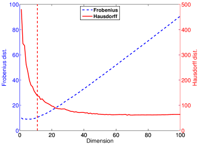

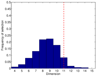
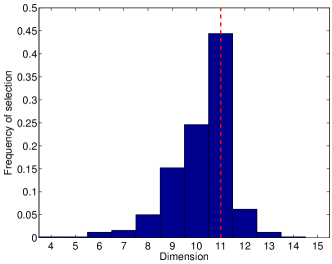
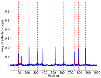
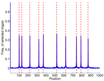
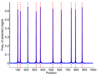
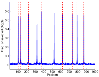
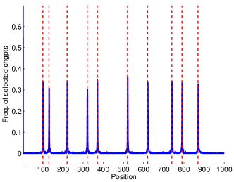

For , notice the high ‘baseline’ level of (wrong) detection of change-points, which is due to a frequent overestimation of the number of change-points, see Figure B.8a.
(Figure B.10c is a copy of Figure 2d, that we repeat here for making comparisons easier.)
